Lecture 3: Optimal Income Taxation (II) - Scholars at Harvard · 2016-09-22 · Lecture 3: Optimal...
53
Lecture 3: Optimal Income Taxation (II) Stefanie Stantcheva Fall 2016 1 52
Transcript of Lecture 3: Optimal Income Taxation (II) - Scholars at Harvard · 2016-09-22 · Lecture 3: Optimal...

Lecture 3: Optimal Income Taxation (II)
Stefanie Stantcheva
Fall 2016
1 52

GOALS OF THIS LECTURE
1) Illustration of structural vs. policy elasticities using the example of thelinear top tax rate.
2) General non-linear tax derivation à la Saez (2001) without income effects.
3) Mechanism Design approach of Mirrlees (1971) and link between thetwo approaches (primitives vs. sufficient stats).
4) Adding income effects.
5) Extension 1: Migration effects
6) Extension 2: Rent-Seeking
2 52

Recap: The Envelope Theorem
When considering a tax change (small), the envelope theorem tells us thatif all is regular, the direct welfare impact of the tax change on agent i isthe mechanical impact on his consumption times marginal utility.
This means behavioral responses (e.g.: the adjustment in labor supply) haveno first-order impact on welfare if they are at the optimum level chosen bythe agent to start with.
The social impact is the mechanical change in consumption times marginalsocial welfare weight.
But the behavioral responses do have a first-order impact on revenues.Those revenues are either rebated or valued at the marginal cost of publicfunds. Either way, this does have a first-order effect on welfare. (When isthis not true?)
3 52

Elasticities: reduced-form vs. structural
Sometimes, it’s enough to express formulas in terms of the reduced-formelasticities, so-called “policy elasticities.”
Other times, interested in decomposing the reduced-form elasticity intoprimitive, structural elasticities, i.e., income and substitution effects.
Depends on the context and what you know from the data.
Let’s illustrate this with the top tax rate derivation.
4 52
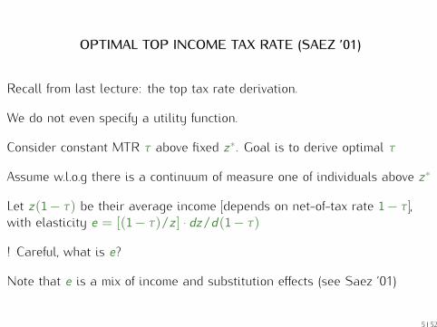
OPTIMAL TOP INCOME TAX RATE (SAEZ ’01)
Recall from last lecture: the top tax rate derivation.
We do not even specify a utility function.
Consider constant MTR τ above fixed z∗. Goal is to derive optimal τ
Assume w.l.o.g there is a continuum of measure one of individuals above z∗
Let z(1− τ) be their average income [depends on net-of-tax rate 1− τ ],with elasticity e = [(1− τ)/z ] · dz/d(1− τ)
! Careful, what is e?
Note that e is a mix of income and substitution effects (see Saez ’01)
5 52

Optimal Top Income Tax Rate (Mirrlees ’71 model)Disposable
Incomec=z-T(z)
Market income z
Top bracket: Slope 1-τ
z*0
Reform: Slope 1-τ−dτ
z*-T(z*)
Source: Diamond and Saez JEP'11

Disposable Income
c=z-T(z)
Market income z
z*
z*-T(z*)
0
Optimal Top Income Tax Rate (Mirrlees ’71 model)
Mechanical tax increase:dτ[z-z*]
Behavioral Response tax loss: τ dz = - dτ e z τ/(1-τ)
z
Source: Diamond and Saez JEP'11
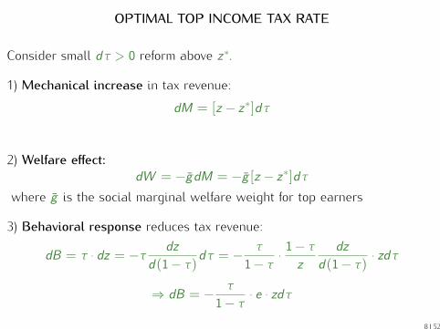
OPTIMAL TOP INCOME TAX RATE
Consider small dτ > 0 reform above z∗.
1) Mechanical increase in tax revenue:dM = [z − z∗]dτ
2) Welfare effect:dW = −gdM = −g [z − z∗]dτ
where g is the social marginal welfare weight for top earners
3) Behavioral response reduces tax revenue:
dB = τ · dz = −τ dz
d(1− τ)dτ = − τ1− τ ·
1− τz
dz
d(1− τ) · zdτ
⇒ dB = − τ1− τ · e · zdτ
8 52
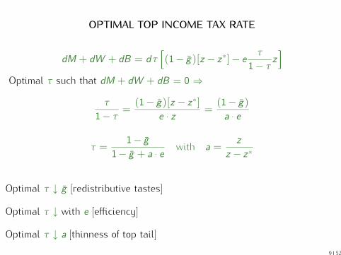
OPTIMAL TOP INCOME TAX RATE
dM + dW + dB = dτ[(1− g)[z − z∗]− e
τ1− τ z
]
Optimal τ such that dM + dW + dB = 0 ⇒
τ1− τ =
(1− g)[z − z∗]
e · z =(1− g)
a · e
τ =1− g
1− g + a · e with a =z
z − z∗
Optimal τ ↓ g [redistributive tastes]
Optimal τ ↓ with e [efficiency]
Optimal τ ↓ a [thinness of top tail]9 52


OPTIMAL TOP TAX RATE – STRUCTURAL FORMULA
Let’s now derive this in terms of the structural elasticities.
!! Change notation to map the Saez (2001) paper (easier for you). z = z∗
and zm = z .
Mechanical revenue effect (M) (at constant incomes) and the welfare effect(W) are naturally the same as above.
Behavioral response: change in marginal tax rate is dτ , change in virtualincome is dR = zdτ .
The change in an individual’s income at income z is:
dz = − ∂z∂(1− τ)dτ +
∂z∂R dR = −(εu(z)z − η(z)z)
dτ1− τ
11 52

OPTIMAL TOP TAX RATE – STRUCTURAL FORMULA
Sum over all individuals earning more than z and multiply by τ to get therevenue change:
B = −(εuzm − ηz)τdτ1− τ
whereεu =
∫ ∞
zεu(z)zh(z)dz/zm
is a weighted average of uncompensated elasticities. εu(z) itself is theaverage uncompensated elasticity over individuals earning z (not necessaryto assume that agents have homogeneous elasticities at given z ).
η =
∫ ∞
zη(z)h(z)dz
is the average income effect for agents with income above z .
12 52

OPTIMAL TOP TAX RATE – STRUCTURAL FORMULASum of B +M +W = 0 means:
τ1− τ =
(1− g)(zm/z − 1)εuzm/z − η
Use Slutsky and definition of a to rearrange:
τ1− τ =
(1− g)
εu + (a− 1)εcComparing to previous formula, we see that the reduced-form andstructural elasticities are linked through:
a · e = εu + (a− 1)εc
!! Careful: still not “primitive” elasticities (haven’t specified utilityfunctions).
13 52

GENERAL NON-LINEAR INCOME TAX T (z)
(1) Lumpsum grant given to everybody equal to −T (0)
(2) Marginal tax rate schedule T ′(z) describing how (a) lump-sum grant istaxed away, (b) how tax liability increases with income
Let H(z) be the income CDF [population normalized to 1] and h(z) itsdensity [endogenous to T (.)]
Let g(z) be the social marginal value of consumption for taxpayers withincome z in terms of public funds [formally g(z) = G ′(u) · uc/λ]: no incomeeffects ⇒
∫g(z)h(z)dz = 1
Redistribution valued ⇒ g(z) decreases with z
Let G (z) the average social marginal value of c for taxpayers with incomeabove z [G (z) =
∫∞z g(s)h(s)ds/(1−H(z))]
14 52

Disposable Incomec=z-T(z)
Pre-tax income zz0
Mechanical tax increase: ddz [1-H(z)]Social welfare effect: -ddz [1-H(z)] G(z)
Behavioral response: z = - d e z/(1-T’(z))Tax loss: T’(z) z h(z)dz= -h(z) e z T’(z)/(1-T’(z)) dzd
z+dz
Small band (z,z+dz): slope 1- T’(z) Reform: slope 1- T’(z)d
ddz
Source: Diamond and Saez JEP'11

GENERAL NON-LINEAR INCOME TAX
Assume away income effects εc = εu = e [Diamond AER’98 shows this isthe key theoretical simplification]
Consider small reform: increase T ′ by dτ in small band z and z + dz
Mechanical effect dM = dzdτ[1−H(z)]
Welfare effect dW = −dzdτ[1−H(z)]G (z)
Behavioral effect: substitution effect δz inside small band [z , z + dz ]:dB = h(z)dz ·T ′ · δz = −h(z)dz ·T ′ · dτ · z · e(z)/(1−T ′)
Optimum dM + dW + dB = 0
16 52

GENERAL NON-LINEAR INCOME TAX
T ′(z) =1−G (z)
1−G (z) + α(z) · e(z)
1) T ′(z) decreases with e(z) (elasticity efficiency effects)
2) T ′(z) decreases with α(z) = (zh(z))/(1−H(z)) (local Paretoparameter)
3) T ′(z) decreases with G (z) (redistributive tastes)
Asymptotics: G (z)→ g , α(z)→ a, e(z) → e ⇒ Recover top rate formulaτ = (1− g)/(1− g + a · e)
17 52

11.
52
2.5
Em
piric
al P
aret
o C
oeffi
cien
t
0 200000 400000 600000 800000 1000000z* = Adjusted Gross Income (current 2005 $)
a=zm/(zm-z*) with zm=E(z|z>z*) alpha=z*h(z*)/(1-H(z*))
Source: Diamond and Saez JEP'11

Negative Marginal Tax Rates Never Optimal
Suppose T ′ < 0 in band [z , z + dz ]
Increase T ′ by dτ > 0 in band [z , z + dz ]: dM + dW > 0 and dB > 0because T ′(z) < 0
⇒ Desirable reform
⇒ T ′(z) < 0 cannot be optimal
EITC schemes are not desirable in Mirrlees ’71 model
19 52

MIRRLEES MODELThe difference to before: we need to specify the structural primitives.
Key simplification is the lack of income effects (Diamond, 1998). We lookinto income effects next time.
Individual utility: c − v(l), l is labor supply.
Skill n is exogenously given, equal to marginal productivity. Earnings arez = nl .
Density is f (n) and CDF F (n) on [0,∞).
Entry into contract theory/mechanism design here: The government doesnot observe skill. Tax is based on income z , T (z).
What happens if we had a tax T (n) available?
Why did we not talk about this in the earlier derivations? Did we ignorethe incentive compatibility constraints?
20 52

Elasticity of labor to taxesRecall we derive elasticities on the linearized budget set. If marginal taxrate is τ , labor supply is: l = l(n(1− τ)). Why the n(1− τ)? Why onlyn(1− τ)?
FOC of the agent for labor supply:
n(1− τ) = v ′(l)
Totally differentiate this (key thing: skill is fixed!) to get elasticity of laborsupply. Also equal to elasticity of income since skill fixed.
d(n(1− τ)) = v ′′(l)dl
⇒ e =dl
d(n(1− tau))
(1− τ)nl
=(1− τ)nlv ′′(l)
=v ′(l)
lv ′′(l)
Is this compensated? uncompensated?21 52

Direct Revelation Mechanism and Incentive Compatibility
We want to max social welfare and have exogenous revenue requirement(non transfer-related E ).
We imagine a direct revelation mechanism. Every agent comes togovernment, reports a type n′. We assign allocations as a function of thereport. c(n′), z(n′), u(n′). Why are we not assigning labor l(n′)?
What are the constraints in this problem?
Feasibility (net resources sum to zero):∫n cnf (n)dn ≥ nlnf (n)dn− E .
Incentive compatibility:
22 52

Direct Revelation Mechanism and Incentive CompatibilityWe want to max social welfare and have exogenous revenue requirement(non transfer-related E ).
We imagine a direct revelation mechanism. Every agent comes togovernment, reports a type n′. We assign allocations as a function of thereport. c(n′), z(n′), u(n′). Why are we not assigning labor l(n′)?
What are the constraints in this problem?
Feasibility (net resources sum to zero):∫n cnf (n)dn ≥ nlnf (n)dn− E .
Incentive compatibility:
c(n)− v
(z(n)
n
)≥ c(n′)− v
(z(n′)
n
)∀n, n′
That’s a lot of constraints!
22 52

Envelope Theorem and First order Approach
Replace the infinity of constraints with agents’ first-order condition. If wetake derivative of utility wrt type n at truth-telling
dundn
=
(c ′(n)− z ′(n)
nv ′(z(n)
n
))dn′
dn+
z(n)
n2 v ′(z(n)
n
)
What if report is optimally chosen?
Envelope condition:dundn
=lnv′(ln)
n
Will replace infinity of constraints.
Is necessary, but what about sufficiency?
23 52

Full Optimization Program
maxcn ,un ,zn
∫nG (un)f (n)dn s.t.
∫ncnf (n)dn ≤
∫nnlnf (n)dn− E
and s.t.dundn = lnv′(ln)n
State variable: un .
Control variables: ln , with cn = un + v(ln).
Why am I suddenly saying ln is a control?
Use optimal control.
24 52

Hamiltonian and Optimal Control
The Hamiltonian is:
H = [G (un) + p · (nln − un − v(ln))]f (n) + φ(n) ·lnv′(ln)
n
p: multiplier on the resource constraint.
φ(n): multiplier on the envelope condition (“costate”). Depends on n!
FOCs:
∂H∂ln
= p · [n− v ′(ln)]f (n) +φ(n)n· [v ′(ln) + lnv
′′(ln)] = 0
∂H∂un
= [G ′(un)− p]f (n) = −dφ(n)dn
Transversality: limn→∞ φ(n) = 0 and φ(0) = 0.
25 52

Rearranging the FOCsTake the integral of the FOC wrt un to solve for φ(n):
−φ(n) =
∫∞
n
[p−G ′(um)]f (m)dm
Integrate this same FOC over the full space, using transversality conditions:
p =
∫ ∞
0G ′(un)f (m)dm
What does this say?
How can we make the tax rate appear? Use the agent’s FOC.
n− v ′(ln) = nT ′(zn)
26 52
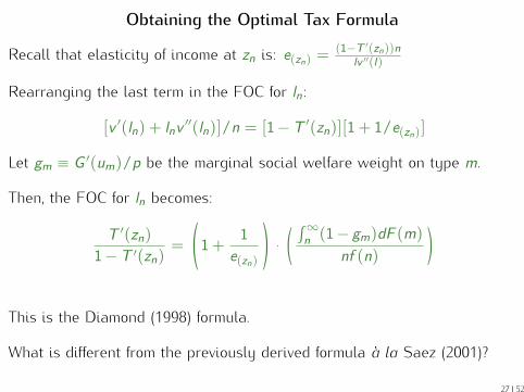
Obtaining the Optimal Tax Formula
Recall that elasticity of income at zn is: e(zn) =(1−T ′(zn))n
lv ′′(l)
Rearranging the last term in the FOC for ln:
[v ′(ln) + lnv′′(ln)]/n = [1−T ′(zn)][1+ 1/e(zn)]
Let gm ≡ G ′(um)/p be the marginal social welfare weight on type m.
Then, the FOC for ln becomes:
T ′(zn)
1−T ′(zn)=
(1+
1e(zn)
)·(∫∞
n (1− gm)dF (m)
nf (n)
)
This is the Diamond (1998) formula.
What is different from the previously derived formula à la Saez (2001)?
27 52

Let’s go from types to observable incomeHow do we go from type distribution to income distribution?
Under linearized tax schedule, earnings are a function zn = nl(n(1− τ)).
How do earnings vary with type?
dzndn
= l + (1− τ)n dl
d(m(1− τ)) = ln · (1+ e(zn))
(intuition?)
Let h(z) be the density of earnings, with CDF H(z). The following relationmust hold:
h(zn)dzn = f (n)dn
f (n) = h(zn)ln(1+ e(zn))⇒ ng(n) = znh(zn)(1+ e(zn))
Let’s substitute income distributions for type distributions in the formula.28 52

Optimal Tax Formula with No Income Effects
T ′(zn)
1−T ′(zn)=
(1+
1e(zn)
)(∫∞n (1− gm)dF (m)
nf (n)
)(primitives)
=1
e(zn)
(1−H(zn)
znh(zn)
)· (1−G (zn)) (incomes)
where:
G (zn) =
∫ ∞n
gmdF (m)
1− F (n)=
∫ ∞zn
gmdH(zm)
1−H(zn)
is the average marginal social welfare weight on individuals with incomeabove zn (change of variables to income distributions in last equality).
Rearrange, use definition of Pareto parameter α(z) = (zh(z))/(1−H(z))to get same formula as before:
T ′(z) =1−G (z)
1−G (z) + α(z) · e(z)
29 52

Recap:
“Mechanism design approach” requires you to specify primitives (utilityfunction, uni-dimensional heterogeneity) as done in Mirrlees (1971).
“Sufficient stats approach” captures arbitrary heterogeneity conditional onz as long as well-behaved elasticities.
Yield same formula if can make the link between types and incomedistributions.
T ′(zn)
1−T ′(zn)=
(1+
1e(zn)
)(∫∞n (1− gm)dF (m)
nf (n)
)(primitives)
=1
e(zn)
(1−H(zn)
znh(zn)
)· (1−G (zn)) (incomes)
30 52

NUMERICAL SIMULATIONS
H(z) [and also G (z)] endogenous to T (.). Calibration method (Saez Restud’01):
Specify utility function (e.g. constant elasticity):
u(c , z) = c − 11+ 1
e
·(zn
)1+ 1e
Individual FOC ⇒ z = n1+e(1−T ′)e
Calibrate the exogenous skill distribution F (n) so that, using actual T ′(.),you recover empirical H(z)
Use Mirrlees ’71 tax formula (expressed in terms of F (n)) to obtain theoptimal tax rate schedule T ′.
31 52

NUMERICAL SIMULATIONS
T ′(z(n))
1−T ′(z(n))=
(1+
1e
)(1
nf (n)
)∫ ∞
n
[1− G ′(u(m))
λ
]f (m)dm,
Iterative Fixed Point method: start with T ′0, compute z0(n) using individualFOC, get T 0(0) using govt budget, compute u0(n), get λ usingλ =
∫G ′(u)f , use formula to estimate T ′1, iterate till convergence
Fast and effective method (Brewer-Saez-Shepard ’10)
32 52
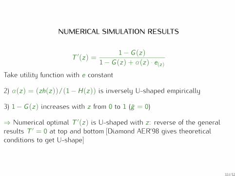
NUMERICAL SIMULATION RESULTS
T ′(z) =1−G (z)
1−G (z) + α(z) · e(z)Take utility function with e constant
2) α(z) = (zh(z))/(1−H(z)) is inversely U-shaped empirically
3) 1−G (z) increases with z from 0 to 1 (g = 0)
⇒ Numerical optimal T ′(z) is U-shaped with z : reverse of the generalresults T ′ = 0 at top and bottom [Diamond AER’98 gives theoreticalconditions to get U-shape]
33 52

0
0.2
0.4
0.6
0.8
1M
argi
nal T
ax R
ate
Utilitarian Criterion, Utility type I
ζc=0.25
ζc=0.5
$0 $100,000 $200,000 $300,000
Wage Income z
FIGURE 5 − Optimal Tax Simulations
0
0.2
0.4
0.6
0.8
1
Mar
gina
l Tax
Rat
e
Utilitarian Criterion, Utility type II
ζc=0.25
ζc=0.5
$0 $100,000 $200,000 $300,000
Wage Income z
0
0.2
0.4
0.6
0.8
1
Mar
gina
l Tax
Rat
e
Rawlsian Criterion, Utility type I
ζc=0.25
ζc=0.5
$0 $100,000 $200,000 $300,000
Wage Income z
0
0.2
0.4
0.6
0.8
1
Mar
gina
l Tax
Rat
e
Rawlsian Criterion, Utility type II
ζc=0.25
ζc=0.5
$0 $100,000 $200,000 $300,000
Wage Income zSource: Saez (2001), p. 224

OPTIMAL NON-LINEAR TAX WITH INCOME EFFECTS
Consider effect of small reform where marginal tax rates increased by dτ in[z∗, z∗ + dz∗].
What are the effects on tax receipts?
Mechanical effect net of welfare loss, M:
Every tax payer with income z above z∗ pays additional dτdz∗, valued at(1− g(z))dτdz∗.
M = dτdz∗∫ ∞
z∗(1− g(z))h(z)dz
35 52


BEHAVIORAL EFFECT PART 1: SUBSTITUTIONIn [z∗, z∗ + dz∗], income changes by dz .
Marginal tax rate changes directly by dτ , but also additionally indirectlyby dT ′(z) = T ′′(z)dz . Why? When is this not the case?
dz = −εc(z)z∗ dτ + dT ′(z)
1−T ′(z)⇒ dz = −εc(z)z
∗ dτ1−T ′(z) + εc(z)z∗T ′′(z)
Define the virtual density: density that would occur at z if tax schedulereplaced by linearized tax schedule. What is the linearized schedule (τ ,R)such that income is (1− τ)z + R?
h∗(z)
1−T ′(z)=
h(z)
1−T ′(z) + εc(z)z∗T ′′(z)
37 52

BEHAVIORAL EFFECT PART 1: SUBSTITUTION
Overall elasticity/substitution effect is then:
E = −εc(z)z∗ T ′(z)
1−T ′(z)h∗(z∗)dτdz∗
Can derive expression without taking into account endogenous (indirect)change in marginal tax rates if use the virtual density instead of true one.
38 52
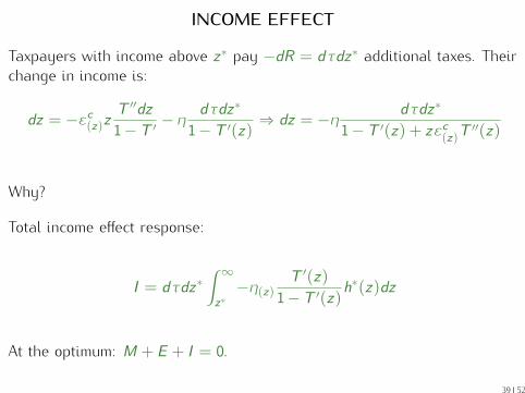
INCOME EFFECT
Taxpayers with income above z∗ pay −dR = dτdz∗ additional taxes. Theirchange in income is:
dz = −εc(z)zT ′′dz
1−T ′− η dτdz∗
1−T ′(z)⇒ dz = −η dτdz∗
1−T ′(z) + zεc(z)T ′′(z)
Why?
Total income effect response:
I = dτdz∗∫ ∞
z∗−η(z)
T ′(z)
1−T ′(z)h∗(z)dz
At the optimum: M + E + I = 0.
39 52

PUTTING THE EFFECTS TOGETHER
T ′(z)
1−T ′(z)=
1εc(z)
(1−H(z∗)
z∗h(z∗)
)
×[∫ ∞
z∗(1− g(z))
h(z)
1−H(z∗)dz +
∫ ∞
z∗−η T ′(z)
1−T ′(z)
h∗(z)
1−H(z∗)dz
]
First-order differential equation. See Saez (2001) Appendix for solution (isstandard).
Change of variable from z to n?
Recall with a linear tax: znzn
=1+εu(zn)
n .
What happens with nonlinear tax? See Saez (2001) Appendix for derivation.
znzn
=1+ εu(zn)
n− zn
T ′′(zn)
1−T ′(zn)εcz(n)
40 52

EXTENSIONS OF THE CORE INCOME TAXATION MODEL
1) Model includes only intensive earnings response. Extensive earningsresponses [entrepreneurship decisions, migration decisions] ⇒ Formulascan be modified
2) Model does not include fiscal externalities: part of the response to dτcomes from income shifting which affects other taxes ⇒ Formulas can bemodified
3) Model does not include classical externalities: (a) charitablecontributions, (b) positive spillovers (trickle down) [top earners underpaid],(c) negative spillovers [top earners overpaid]
Classical general equilibrium effects on prices are NOT externalities anddo not affect formulas [Diamond-Mirrlees AER ’71, Saez JpubE ’04]
41 52

EXTENSION 1: MIGRATION EFFECTS
Tax rates may affect migration (evidence on this next time).
Migration issues may be particularly important at the top end (brain drain).
Some theory papers (Mirrlees ’82, Lehmann-Simula QJE’14). Here:Simplified Mirrlees (1982) model.
Earnings z are fixed, conditional on residence.
P(c|z) is number of residents earning z when disposable income is c , withc = z −T (z).
Consider small tax reform dT (z) for those earning z .
What is migration responding to? Marginal taxes?
42 52

ELASTICITY OF MIGRATION TO TAXES
Mechanical effect net of welfare is: M +W = (1− g(z))P(c|z)dT .
Why? Where is utility effect of changing country induced by taxes?
Migration responds to average taxes (or total taxes, since income fixed).
ηm(z) =∂P(c |z)∂c
z −T (z)
P(c |z)
Fiscal cost of raising taxes by dT (z) is: B = − T (z)z−T (z)
· P(c|z) · ηm
Optimal tax is where M +W + B = 0:
T (z)
z −T (z)=
1ηm(z)
· (1− g(z))
What determines the elasticity ηm(z)?
43 52

MIGRATION EFFECTS IN THE STANDARD MODEL
ηm(z) depends on size of jurisdiction: large for cities, zero worldwide ⇒(1) Redistribution easier in large jurisdictions, (2) Tax coordination acrosscountries increases ability to redistribute (big issue currently in EU), (3)visa system, cost of migration, ...
Top revenue maximizing tax rate formula (Brewer-Saez-Shepard ’10):
τ =1
1+ a · e + ηm
where ηm is the elasticity of top earners to disposable income.
44 52

EXTENSION 2: RENT SEEKING EFFECTS
Pay may not be equal to the marginal economic product for top incomeearners. Why? Overpaid or underpaid?
Piketty, Saez, and Stantcheva (2014) “A Tale of Three Elasticities.”
Actual output is y , but individual only receives share η of actual output. Toincrease either productive effort or rent-seeking, effort is required.
ui (c ,η, y) = c − hi (y)− ki (η)
Define bargained earnings: b = (η− 1)y .
Average bargaining is E (b), extracted equally from everyone else (goodassumption?) Means E (b) can be perfectly canceled by −T (0).
45 52

RENT SEEKING ELASTICITIESGiven tax, individual maximizes:
ui (c , y ,η) = η · y −T (η · y)− hi (y)− ki (η)What will yi and ηi depend on?
Average reported income, productive income and bargained earnings in thetop bracket:
z(1− τ), y(1− τ), η(1− τ)
Total compensation elasticity e: e = 1−τz
dzd(1−τ) (what is it driven by?)
Real labor supply elasticity ey : ey = 1−τy
dyd(1−τ) ≥ 0.
Thus the bargaining elasticity component eb = dbd(1−τ)
1−τz = s · e with
s = db/d(1−τ)dz/d(1−τ)
s and eb positive if η > 1.46 52
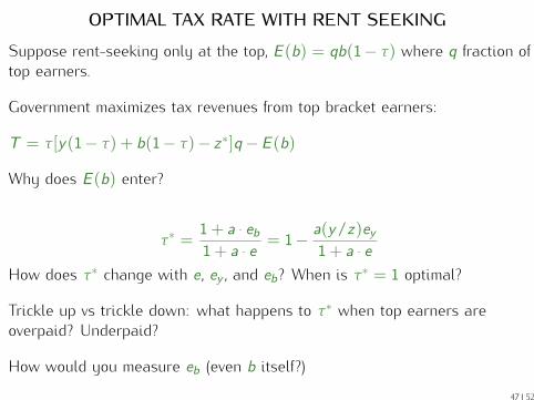
OPTIMAL TAX RATE WITH RENT SEEKINGSuppose rent-seeking only at the top, E (b) = qb(1− τ) where q fraction oftop earners.
Government maximizes tax revenues from top bracket earners:
T = τ[y(1− τ) + b(1− τ)− z∗]q − E (b)
Why does E (b) enter?
τ∗ = 1+ a · eb1+ a · e = 1− a(y/z)ey
1+ a · eHow does τ∗ change with e , ey , and eb? When is τ∗ = 1 optimal?
Trickle up vs trickle down: what happens to τ∗ when top earners areoverpaid? Underpaid?
How would you measure eb (even b itself?)
47 52

REFERENCES (for lectures 2 and 3)
Akerlof, G. “The Economics of Tagging as Applied to the Optimal Income Tax,Welfare Programs, and Manpower Planning”, American Economic Review, Vol. 68,1978, 8-19. (web)
Atkinson, A.B. and J. Stiglitz “The design of tax structure: Direct versus indirecttaxation”, Journal of Public Economics, Vol. 6, 1976, 55-75. (web)
Besley, T. and S. Coate “Workfare versus Welfare: Incentives Arguments for WorkRequirements in Poverty-Alleviation Programs”, American Economic Review, Vol.82, 1992, 249-261. (web)
Boskin, M. and E. Sheshinski “Optimal tax treatment of the family: Marriedcouples”, Journal of Public Economics, Vol. 20, 1983, 281-297 (web)
Brewer, M., E. Saez, and A. Shephard “Means Testing and Tax Rates on Earnings”,in The Mirrlees Review: Reforming the Tax System for the 21st Century, OxfordUniversity Press, 2010. (web)
48 52

Cremer, H., F. Gahvari, and N. Ladoux “Externalities and optimal taxation”, Journalof Public Economics, Vol. 70, 1998, 343-364. (web)
Deaton, A. “Optimal Taxes and the Structure of Preferences”, Econometrica, Vol. 49,1981, 1245-1260 (web)
Diamond, P. “A many-person Ramsey tax rule”, Journal of Public Economics, Vol.4,1975, 335-342. (web)
Diamond, P. “Income Taxation with Fixed Hours of Work”Journal of PublicEconomics, Vol. 13, 1980, 101-110. (web)
Diamond, P. “Optimal Income Taxation: An Example with a U-Shaped Pattern ofOptimal Marginal Tax Rates”, American Economic Review, Vol. 88, 1998, 83-95.(web) Skim this for historical reasons.
Diamond, P. and E. Saez “From Basic Research to Policy Recommendations:The Case for a Progressive Tax”, Journal of Economic Perspectives, 25(4), 2011,165-190. (web)
Edgeworth, F. “The Pure Theory of Taxation”, The Economic Journal, Vol. 7, 1897,550-571. (web)
49 52

Kaplow, L. “On the undesirability of commodity taxation even when income taxationis not optimal”, Journal of Public Economics, Vol. 90, 2006, 1235-1250. (web)
Kaplow, L. The Theory of Taxation and Public Economics. Princeton UniversityPress, 2008.
Kaplow, L. and S. Shavell “Any Non-welfarist Method of Policy AssessmentViolates the Pareto Principle,” Journal of Political Economy, 109(2), (April 2001),281-286 (web)
Kleven, H., C. Kreiner and E. Saez “The Optimal Income Taxation of Couples”,Econometrica, Vol. 77, 2009, 537-560. (web)
Laroque, G. “Indirect Taxation is Superfluous under Separability and TasteHomogeneity: A Simple Proof”, Economic Letters, Vol. 87, 2005, 141-144. (web)
Lehmann, E., L. Simula, A. Trannoy “Tax Me if You Can! Optimal Nonlinear IncomeTax between Competing Governments,” Quarterly Journal of Economics 129(4),2014, 1995-2030. (web)
50 52

Mankiw, G. and M. Weinzierl “The Optimal Taxation of Height: A Case Study ofUtilitarian Income Redistribution”, AEJ: Economic Policy, Vol. 2, 2010, 155-176.(web)
Mirrlees, J. “An Exploration in the Theory of Optimal Income Taxation”, Reviewof Economic Studies, Vol. 38, 1971, 175-208. (web) Read it for historicalreasons, it is not very easy to follow.
Mirrlees, J. “Migration and Optimal Income Taxes”, Journal of Public Economics,Vol. 18, 1982, 319-341. (web)
Nichols, A. and R. Zeckhauser“Targeting Transfers Through Restrictions onRecipients”, American Economic Review, Vol. 72, 1982, 372-377. (web)
Piketty, Thomas and Emmanuel Saez “Optimal Labor Income Taxation,”Handbook of Public Economics, Volume 5, Amsterdam: Elsevier-North Holland,2013. (web)
Piketty, Thomas, Emmanuel Saez, and Stefanie Stantcheva "Optimal Taxation ofTop Labor Incomes: A Tale of Three Elasticities", American Economic Journal:Economic Policy, 6(1), 2014, 230-271 (web)
51 52

Sadka, E. “On Income Distribution, Incentives Effects and Optimal IncomeTaxation”, Review of Economic Studies, Vol. 43, 1976, 261-268. (web)
Saez, E. “Using Elasticities to Derive Optimal Income Tax Rates”, Review ofEconomics Studies, Vol. 68, 2001, 205-229. (web)
Saez, E. “The Desirability of Commodity Taxation under Non-linear IncomeTaxation and Heterogeneous Tastes”, Journal of Public Economics, Vol. 83, 2002,217-230. (web)
Sandmo, A. “Optimal Taxation in the Presence of Externalities”, The SwedishJournal of Economics, Vol. 77, 1975, 86-98. (web)
Seade, Jesus K. “On the shape of optimal tax schedules.” Journal of publicEconomics 7.2 (1977): 203-235. (web)
Stiglitz, J. “Self-selection and Pareto Efficient Taxation”, Journal of PublicEconomics, Vol. 17, 1982, 213-240. (web)
52 52