1

Lecture 3 - Conservation Equations

Applied Computational Fluid Dynamics

Instructor: André Bakker

http://www.bakker.org© André Bakker (2002-2006)

2

• The governing equations include the following conservation laws of physics:– Conservation of mass.– Newton’s second law: the change of momentum equals the sum of

forces on a fluid particle.– First law of thermodynamics (conservation of energy): rate of change

of energy equals the sum of rate of heat addition to and work done on fluid particle.

• The fluid is treated as a continuum. For length scales of, say, 1µm and larger, the molecular structure and motions may be ignored.

Governing equations

3

Lagrangian vs. Eulerian description

A fluid flow field can be thought of as being comprised of a large number of finite sized fluid particles which have mass, momentum, internal energy, and other properties. Mathematical laws can then be written for each fluid particle. This is the Lagrangian description of fluid motion.

Another view of fluid motion is the Eulerian description. In the Eulerian description of fluid motion, we consider how flow properties change at a fluid element that is fixed in space and time (x,y,z,t), rather than following individual fluid particles.

Governing equations can be derived using each method and converted to the other form.

4

Fluid element and properties

• The behavior of the fluid is described in terms of macroscopic properties:– Velocity u.– Pressure p.– Density ρ.– Temperature T.– Energy E.

• Typically ignore (x,y,z,t) in the notation.• Properties are averages of a sufficiently

large number of molecules.• A fluid element can be thought of as the

smallest volume for which the continuum assumption is valid.

xy

z

δδδδyδδδδx

δδδδz(x,y,z)

Fluid element for conservation laws

Faces are labeled North, East, West,

South, Top and Bottom

1 1

2 2W E

p pp p x p p x

x xδ δ∂ ∂= − = +

∂ ∂

Properties at faces are expressed as first

two terms of a Taylor series expansion,

e.g. for p : and

5

Mass balance

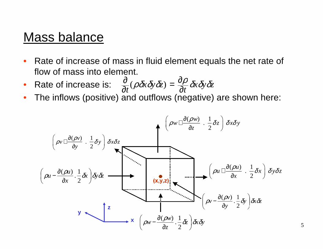
• Rate of increase of mass in fluid element equals the net rate offlow of mass into element.

• Rate of increase is:• The inflows (positive) and outflows (negative) are shown here:

zyxt

zyxt

δδδρδδρδ ∂∂=∂

∂ )(

xy

z

( ) 1.

2

ww z x y

z

ρρ δ δ δ∂ + ∂

( ) 1.

2

vv y x z

y

ρρ δ δ δ ∂+ ∂

zyxx

uu δδδρρ

∂∂−

21

.)(

zxyy

vv δδδρρ

∂∂−

21

.)(

yxzz

ww δδδρρ

∂∂−

21

.)(

( ) 1.

2

uu x y z

x

ρρ δ δ δ∂ + ∂

6

Continuity equation

• Summing all terms in the previous slide and dividing by the volume δxδyδz results in:

• In vector notation:

• For incompressible fluids ∂ρ /∂ t = 0, and the equation becomes: div u = 0.

• Alternative ways to write this: and

0)()()( =∂∂+∂

∂+∂∂+∂

∂zw

yv

xu

tρρρρ

0)( =+∂∂ uρρ div

tChange in density Net flow of mass across boundaries

Convective term

0=∂∂+∂

∂+∂∂

zw

yv

xu 0=∂

∂

i

ixu

7

Different forms of the continuity equation

formonConservati

formIntegral

dVt SV

0=⋅+∂∂

∫∫∫∫∫ dSUρρ

formonconservatiNon

formIntegral

dVDt

D

V

−

=∫∫∫ 0ρ

formonConservati

formalDifferentit

0)( =⋅∇+∂∂

Uρρ

formonconservatiNon

formalDifferentiDt

D

−

=⋅∇+ 0UρρInfinitesimally small

element fixed in space

Infinitesimally small fluid element of fixed mass (“fluid particle”) moving with the flow

Finite control volumefixed in space

Finite control volume fixed mass moving with flow

U

8

Rate of change for a fluid particle

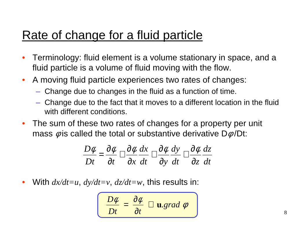
• Terminology: fluid element is a volume stationary in space, and a fluid particle is a volume of fluid moving with the flow.

• A moving fluid particle experiences two rates of changes:– Change due to changes in the fluid as a function of time.– Change due to the fact that it moves to a different location in the fluid

with different conditions.

• The sum of these two rates of changes for a property per unit mass φ is called the total or substantive derivative Dφ /Dt:

• With dx/dt=u, dy/dt=v, dz/dt=w, this results in:

dt

dz

zdt

dy

ydt

dx

xtDt

D

∂∂+

∂∂+

∂∂+

∂∂= φφφφφ

φφφgrad

tDt

D.u+

∂∂=

9

Rate of change for a stationary fluid element

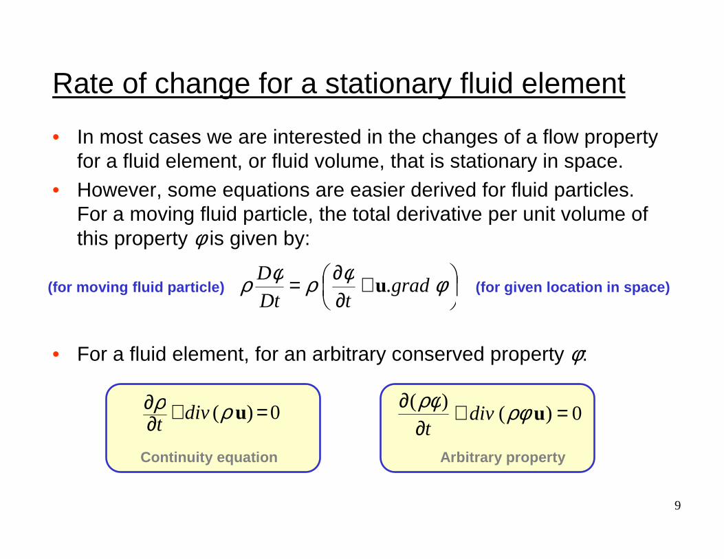
• In most cases we are interested in the changes of a flow property for a fluid element, or fluid volume, that is stationary in space.

• However, some equations are easier derived for fluid particles. For a moving fluid particle, the total derivative per unit volume of this property φ is given by:

• For a fluid element, for an arbitrary conserved property φ :

+∂∂= φφρφρ grad

tDt

D.u

0)( =+∂∂ uρρ div

t 0)()( =+

∂∂

uρφρφdiv

tContinuity equation Arbitrary property

(for moving fluid particle) (for given location in space)

10

Dt

Ddiv

tgrad

tdiv

t

φρρρφφφρρφρφ =

+∂∂+

+∂∂=+

∂∂

)(.)()(

uuu

zero because of continuity

Dt

Ddiv

t

φρρφρφ =+∂

∂)(

)(u

Rate of increase ofφφφφ of fluid element

Net rate of flow ofφφφφ out of fluid element

Rate of increase of φφφφ for a fluid particle=

Fluid particle and fluid element

• We can derive the relationship between the equations for a fluidparticle (Lagrangian) and a fluid element (Eulerian) as follows:

11

To remember so far

• We need to derive conservation equations that we can solve to calculate fluid velocities and other properties.

• These equations can be derived either for a fluid particle that is moving with the flow (Lagrangian) or for a fluid element that isstationary in space (Eulerian).

• For CFD purposes we need them in Eulerian form, but (according to the book) they are somewhat easier to derive in Lagrangian form.

• Luckily, when we derive equations for a property φ in one form, we can convert them to the other form using the relationship shown on the bottom in the previous slide.

12

Relevant entries for Φ

x-momentum

u

Dt

Duρ

)()(

uudivt

u ρρ +∂

∂

y-momentum

v

Dt

Dvρ

)()(

uvdivt

v ρρ +∂

∂

z-momentum

w

Dt

Dwρ

)()(

uwdivt

w ρρ +∂

∂

Energy

E

Dt

DEρ

)()(

uEdivt

E ρρ +∂

∂

13

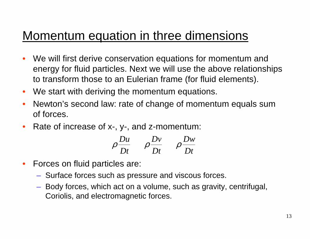
Momentum equation in three dimensions

• We will first derive conservation equations for momentum and energy for fluid particles. Next we will use the above relationships to transform those to an Eulerian frame (for fluid elements).

• We start with deriving the momentum equations.• Newton’s second law: rate of change of momentum equals sum

of forces.• Rate of increase of x-, y-, and z-momentum:

• Forces on fluid particles are:– Surface forces such as pressure and viscous forces.– Body forces, which act on a volume, such as gravity, centrifugal,

Coriolis, and electromagnetic forces.

Dt

Dw

Dt

Dv

Dt

Du ρρρ

14

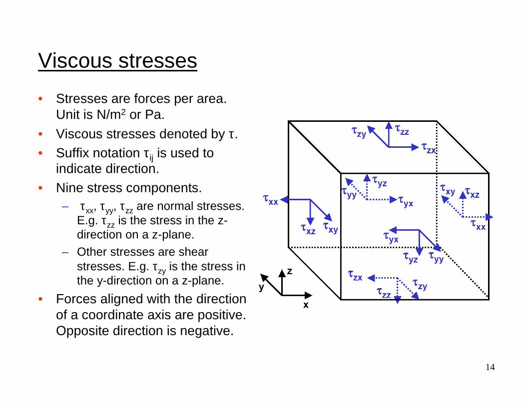
Viscous stresses

• Stresses are forces per area. Unit is N/m2 or Pa.

• Viscous stresses denoted by τ.• Suffix notation τij is used to

indicate direction.• Nine stress components.

– τxx, τyy, τzz are normal stresses. E.g. τzz is the stress in the z-direction on a z-plane.

– Other stresses are shear stresses. E.g. τzy is the stress in the y-direction on a z-plane.

• Forces aligned with the direction of a coordinate axis are positive. Opposite direction is negative.

15

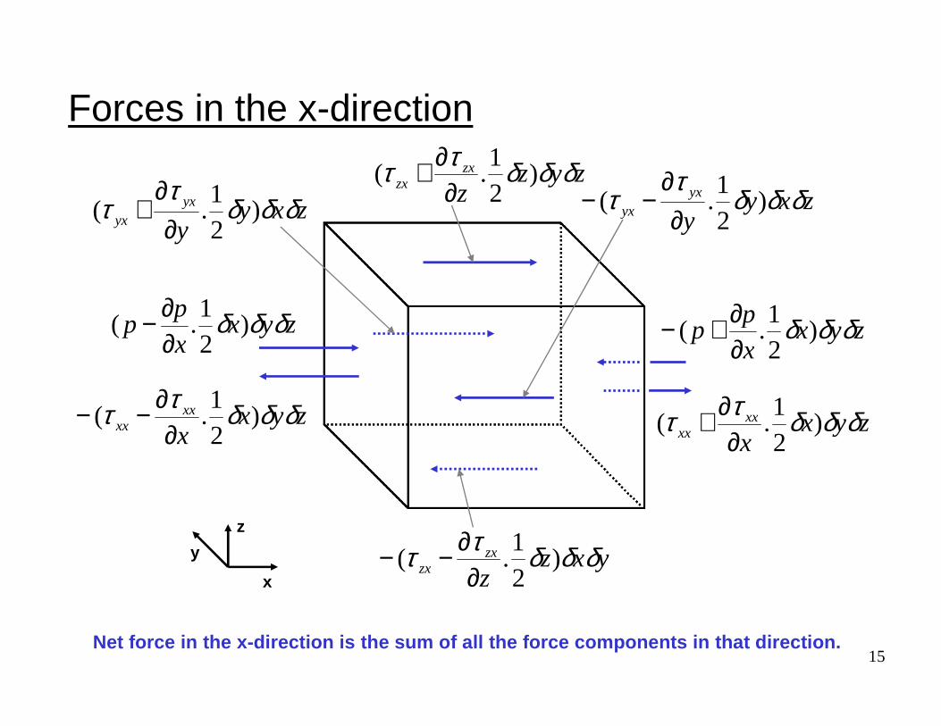
Forces in the x-direction

x

z

y

zyxx

pp δδδ )

21

.(∂∂+−zyx

x

pp δδδ )

21

.(∂∂−

zyzzzx

zx δδδττ )21

.(∂

∂+

yxzzzx

zx δδδττ )21

.(∂

∂−−

zxyyyx

yx δδδτ

τ )21

.(∂

∂−−zxy

yyx

yx δδδτ

τ )21

.(∂

∂+

zyxxxx

xx δδδττ )21

.(∂

∂−− zyxxxx

xx δδδττ )21

.(∂

∂+

Net force in the x-direction is the sum of all the force components in that direction.

16

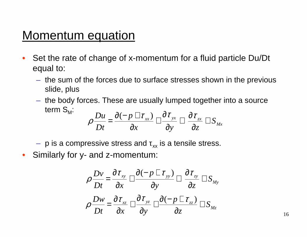
Momentum equation

• Set the rate of change of x-momentum for a fluid particle Du/Dt equal to:– the sum of the forces due to surface stresses shown in the previous

slide, plus– the body forces. These are usually lumped together into a source

term SM:

– p is a compressive stress and τxx is a tensile stress.

• Similarly for y- and z-momentum:

Mxzxyxxx Szyx

p

Dt

Du +∂

∂+∂

∂+

∂+−∂= τττρ )(

Myzyyyxy Szy

p

xDt

Dv +∂

∂+

∂+−∂

+∂

∂=

τττρ

)(

Mzzzyzxz S

z

p

yxDt

Dw +∂

+−∂+∂

∂+

∂∂= )( τττρ

17

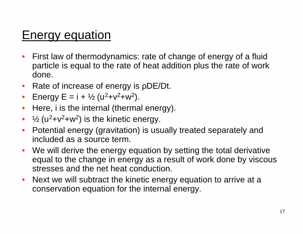
Energy equation

• First law of thermodynamics: rate of change of energy of a fluidparticle is equal to the rate of heat addition plus the rate of work done.

• Rate of increase of energy is ρDE/Dt.• Energy E = i + ½ (u2+v2+w2). • Here, i is the internal (thermal energy).• ½ (u2+v2+w2) is the kinetic energy.• Potential energy (gravitation) is usually treated separately and

included as a source term.• We will derive the energy equation by setting the total derivative

equal to the change in energy as a result of work done by viscous stresses and the net heat conduction.

• Next we will subtract the kinetic energy equation to arrive at aconservation equation for the internal energy.

18

zyxx

upup δδδ )

21

.)(

(∂

∂+−

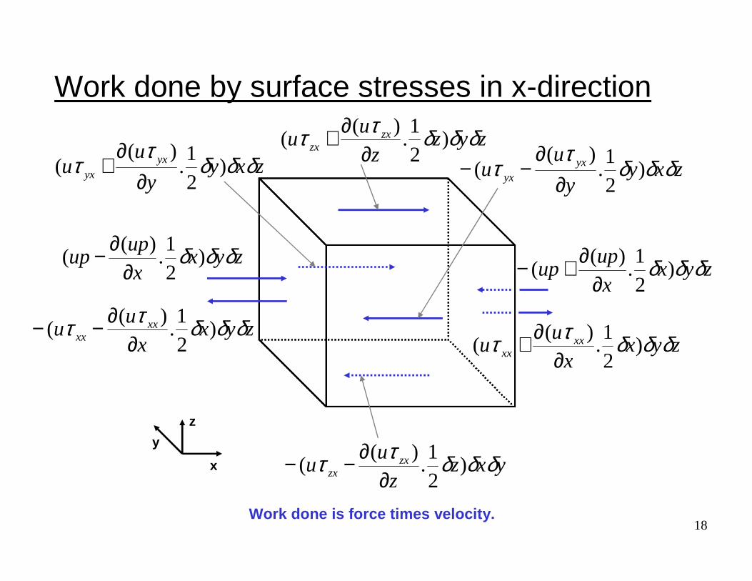
Work done by surface stresses in x-direction

x

z

y

zyxx

upup δδδ )

21

.)(

(∂

∂−

zyzz

uu zx

zx δδδττ )21

.)(

(∂

∂+

yxzz

uu zx

zx δδδττ )21

.)(

(∂

∂−−

zxyy

uu yx

yx δδδτ

τ )21

.)(

(∂

∂−−zxy

y

uu yx

yx δδδτ

τ )21

.)(

(∂

∂+

zyxx

uu xx

xx δδδττ )21

.)(

(∂

∂−−zyx

x

uu xx

xx δδδττ )21

.)(

(∂

∂+

Work done is force times velocity.

19

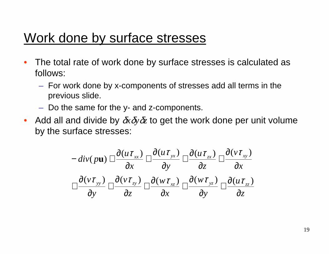
Work done by surface stresses

• The total rate of work done by surface stresses is calculated asfollows:– For work done by x-components of stresses add all terms in the

previous slide.– Do the same for the y- and z-components.

• Add all and divide by δxδyδz to get the work done per unit volume by the surface stresses:

z

u

y

w

x

w

z

v

y

v

x

v

z

u

y

u

x

updiv

zzyzxzzyyy

xyzxyxxx

∂∂+

∂∂

+∂

∂+∂

∂+

∂∂

+

∂∂

+∂

∂+∂

∂+

∂∂+−

)()()()()(

)()()()()(

τττττ

ττττu

20

Energy flux due to heat conduction

x

z

y

yxzz

qq z

z δδδ )21

.(∂∂+

yxzz

qq z

z δδδ )21

.(∂∂−

zyxx

qq x

x δδδ )21

.(∂∂+zyx

x

qq x

x δδδ )21

.(∂∂−

zxyy

qq y

y δδδ )21

.(∂∂

+

zxyy

qq y

y δδδ )21

.(∂∂

−

The heat flux vector q has three components, q x, qy, and q z.

21

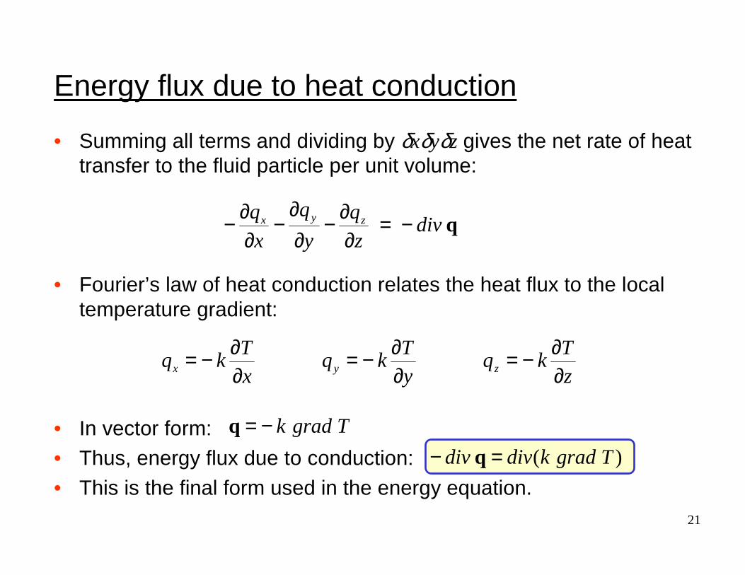
Energy flux due to heat conduction

• Summing all terms and dividing by δxδyδz gives the net rate of heat transfer to the fluid particle per unit volume:

• Fourier’s law of heat conduction relates the heat flux to the local temperature gradient:

• In vector form:• Thus, energy flux due to conduction: • This is the final form used in the energy equation.

qdivz

q

y

q

x

q zyx −=∂∂−

∂∂

−∂∂−

z

Tkq

y

Tkq

x

Tkq zyx ∂

∂−=∂∂−=

∂∂−=

Tgradk−=q

)( Tgradkdivdiv =− q

22

Energy equation

• Setting the total derivative for the energy in a fluid particle equal to the previously derived work and energy flux terms, results inthe following energy equation:

• Note that we also added a source term SE that includes sources (potential energy, sources due to heat production from chemical reactions, etc.).

E

zzyzxzzyyy

xyzxyxxx

STgradkdiv

z

u

y

w

x

w

z

v

y

v

x

v

z

u

y

u

x

updiv

Dt

DE

++

∂∂+

∂∂

+∂

∂+∂

∂+

∂∂

+

∂∂

+∂

∂+∂

∂+

∂∂+−=

)(

)()()()()(

)()()()()(

τττττ

ττττρ u

23

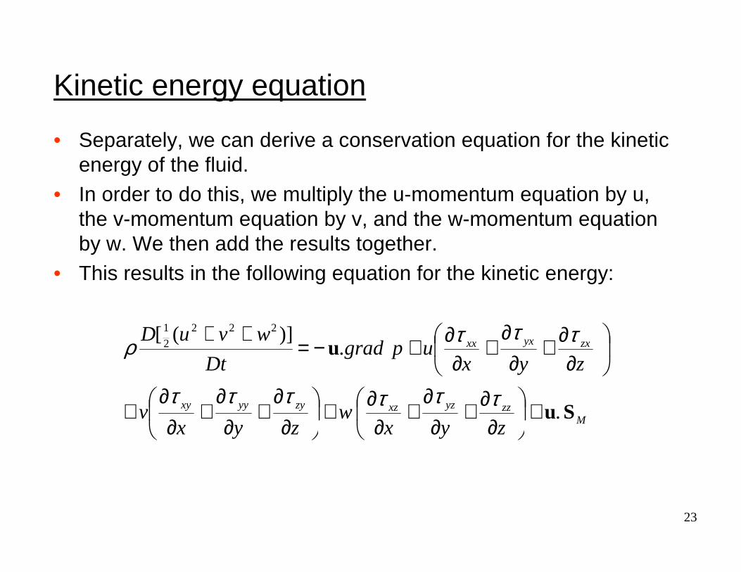
Kinetic energy equation

• Separately, we can derive a conservation equation for the kinetic energy of the fluid.

• In order to do this, we multiply the u-momentum equation by u, the v-momentum equation by v, and the w-momentum equation by w. We then add the results together.

• This results in the following equation for the kinetic energy:

Mzzyzxzzyyyxy

zxyxxx

zyxw

zyxv

zyxupgrad

Dt

wvuD

Su

u

.

.)]([ 222

2

1

+

∂∂+

∂∂

+∂

∂+

∂∂

+∂

∂+

∂∂

+

∂∂+

∂∂

+∂

∂+−=++

ττττττ

τττρ

24

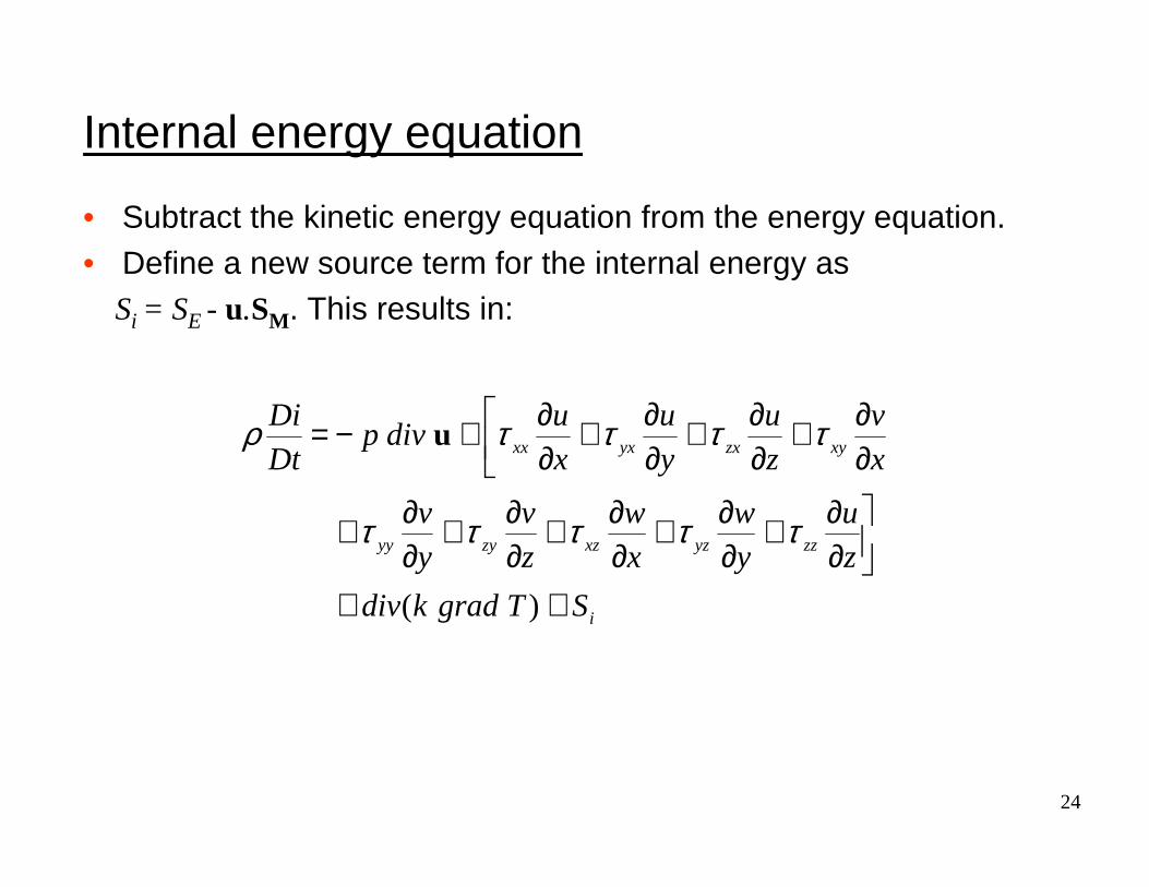
Internal energy equation

• Subtract the kinetic energy equation from the energy equation.• Define a new source term for the internal energy as

Si = SE - u.SM. This results in:

i

zzyzxzzyyy

xyzxyxxx

STgradkdiv

z

u

y

w

x

w

z

v

y

v

x

v

z

u

y

u

x

udivp

Dt

Di

++

∂∂+

∂∂+

∂∂+

∂∂+

∂∂+

∂∂+

∂∂+

∂∂+

∂∂+−=

)(

τττττ

ττττρ u

25

Enthalpy equation

• An often used alternative form of the energy equation is the total enthalpy equation.– Specific enthalpy h = i + p/ρ.– Total enthalpy h0 = h + ½ (u2+v2+w2) = E + p/ρ.

00

( )( ) ( )

( ) ( )( ) ( )

( ) ( ) ( )( ) ( )

yx xyxx zx

yy zy yzxz zz

h

hdiv h div k grad T

tu vu u

x y z x

v v ww u

y z x y z

S

ρ ρ

τ ττ τ

τ τ ττ τ

∂ + =∂

∂ ∂∂ ∂+ + + + ∂ ∂ ∂ ∂

∂ ∂ ∂ ∂ ∂+ + + + + ∂ ∂ ∂ ∂ ∂

+

u

26

Equations of state

• Fluid motion is described by five partial differential equations for mass, momentum, and energy.

• Amongst the unknowns are four thermodynamic variables: ρ, p, i, and T.

• We will assume thermodynamic equilibrium, i.e. that the time it takes for a fluid particle to adjust to new conditions is short relative to the timescale of the flow.

• We add two equations of state using the two state variables ρ and T: p=p(ρ,T) and i=i(ρ,T).

• For a perfect gas, these become: p=ρ RT and i=CvT.• At low speeds (e.g. Ma < 0.2), the fluids can be considered

incompressible. There is no linkage between the energy equation,and the mass and momentum equation. We then only need to solve for energy if the problem involves heat transfer.

27

Viscous stresses

• A model for the viscous stresses τij is required.• We will express the viscous stresses as functions of the local

deformation rate (strain rate) tensor.• There are two types of deformation:

– Linear deformation rates due to velocity gradients.• Elongating stress components (stretching).

• Shearing stress components.

– Volumetric deformation rates due to expansion or compression.

• All gases and most fluids are isotropic: viscosity is a scalar.• Some fluids have anisotropic viscous stress properties, such as

certain polymers and dough. We will not discuss those here.

28

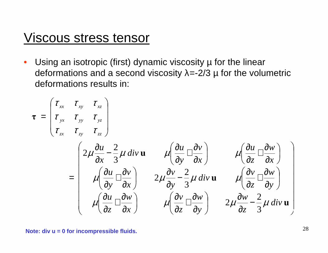
Viscous stress tensor

−∂∂

∂∂+

∂∂

∂∂+

∂∂

∂∂+

∂∂−

∂∂

∂∂+

∂∂

∂∂+

∂∂

∂∂+

∂∂−

∂∂

=

=

u

u

u

τ

divz

w

y

w

z

v

x

w

z

uy

w

z

vdiv

y

v

x

v

y

ux

w

z

u

x

v

y

udiv

x

u

zzzyzx

yzyyyx

xzxyxx

µµµµ

µµµµ

µµµµ

τττττττττ

32

2

32

2

32

2

• Using an isotropic (first) dynamic viscosity µ for the linear deformations and a second viscosity λ=-2/3 µ for the volumetric deformations results in:

Note: div u = 0 for incompressible fluids.

29

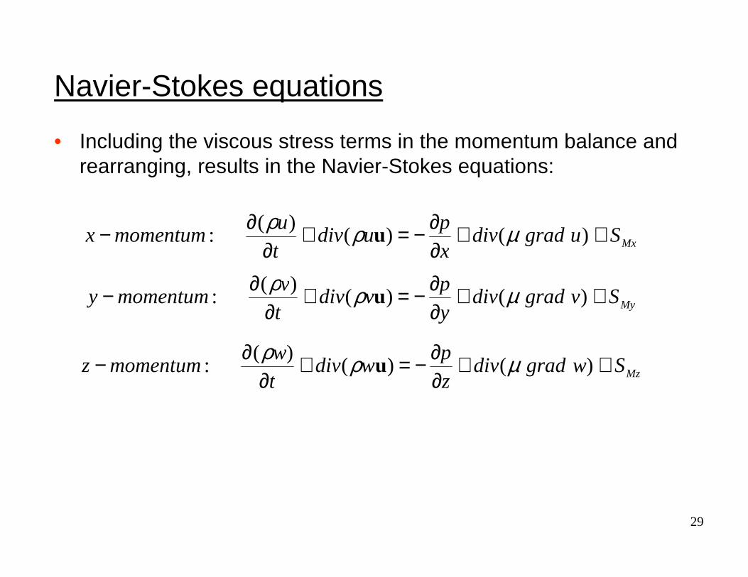
Navier-Stokes equations

• Including the viscous stress terms in the momentum balance and rearranging, results in the Navier-Stokes equations:

MxSugraddivx

pudiv

t

umomentumx ++

∂∂−=+

∂∂− )()(

)(: µρρ

u

MySvgraddivy

pvdiv

t

vmomentumy ++

∂∂−=+

∂∂− )()(

)(: µρρ

u

MzSwgraddivz

pwdiv

t

wmomentumz ++

∂∂−=+

∂∂− )()(

)(: µρρ

u

30

Viscous dissipation

• Similarly, substituting the stresses in the internal energy equation and rearranging results in:

• Here Φ is the viscous dissipation term. This term is always positive and describes the conversion of mechanical energy to heat.

iSTgradkdivdivpidivt

ienergyInternal +Φ++−=+

∂∂

)()()(

: uuρρ

2

22

2222

)(32

2

udivy

w

z

v

x

w

z

u

x

v

y

u

z

w

y

v

x

u

µ

µ

−

∂∂+

∂∂+

∂∂+

∂∂+

∂∂+

∂∂+

∂∂+

∂∂+

∂∂=Φ

31

Summary of equations in conservation form

0)(: =+∂∂

uρρdiv

tMass

MxSugraddivx

pudiv

t

umomentumx ++

∂∂−=+

∂∂− )()(

)(: µρρ

u

MySvgraddivy

pvdiv

t

vmomentumy ++

∂∂−=+

∂∂− )()(

)(: µρρ

u

MzSwgraddivz

pwdiv

t

wmomentumz ++

∂∂−=+

∂∂− )()(

)(: µρρ

u

iSTgradkdivdivpidivt

ienergyInternal +Φ++−=+

∂∂

)()()(

: uuρρ

TCiandRTpgasperfectforge

TiiandTppstateofEquations

v====

ρρρ

:..

),(),(:

32

• The system of equations is now closed, with seven equations for seven variables: pressure, three velocity components, enthalpy, temperature, and density.

• There are significant commonalities between the various equations. Using a general variable φ, the conservative form of all fluid flow equations can usefully be written in the following form:

• Or, in words:

General transport equations

( ) ( ) ( ) φφρφρφSgraddivdiv

t+Γ=+

∂∂

u

Rate of increaseof φφφφ of fluid

element

Net rate of flowof φφφφ out of

fluid element(convection)

Rate of increaseof φφφφ due to diffusion

Rate of increase of φφφφ due to

sources=+ +

33

Integral form

• The key step of the finite volume method is to integrate the differential equation shown in the previous slide, and then to apply Gauss’divergence theorem, which for a vector a states:

• This then leads to the following general conservation equation in integral form:

• This is the actual form of the conservation equations solved by finite volume based CFD programs to calculate the flow pattern and associated scalar fields.

∫∫ ⋅=ACV

dAdVdiv ana

dVSdAgraddAdVt CVAACV

∫∫∫∫ +Γ⋅=⋅+

∂∂

φφρφρφ )()( nun

Rate of increase

of φφφφ

Net rate of decrease of φφφφ due

to convectionacross boundaries

Net rate of increase of φφφφ due

to diffusionacross boundaries

Net rate of creation

of φφφφ=+ +