Lecture 3: Characteristics and Partitioning of Contaminantsbaiyu/ENGI 9621_files/Lecture 3.pdf ·...
44
Spring 2015 Faculty of Engineering & Applied Science Lecture 3: Characteristics and Partitioning of Contaminants 1 9621 – Soil Remediation Engineering
Transcript of Lecture 3: Characteristics and Partitioning of Contaminantsbaiyu/ENGI 9621_files/Lecture 3.pdf ·...

Spring 2015 Faculty of Engineering & Applied Science
Lecture 3: Characteristics and Partitioning of Contaminants
1
9621 – Soil Remediation Engineering
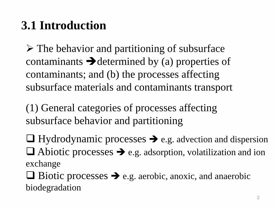
The behavior and partitioning of subsurface contaminants determined by (a) properties of contaminants; and (b) the processes affecting subsurface materials and contaminants transport (1) General categories of processes affecting subsurface behavior and partitioning
3.1 Introduction
Hydrodynamic processes e.g. advection and dispersion Abiotic processes e.g. adsorption, volatilization and ion exchange Biotic processes e.g. aerobic, anoxic, and anaerobic biodegradation
2

(2) Classification of soil contaminants
By definition, soil contaminants can be classified into
Organic compounds that contain organic carbon e.g. petroleum products (gasoline, kerosene, diesel fuel…), polynuclear aromatic hydrocarbons (PAHs) Inorganic those that contain no organic carbon (mainly metal contaminants) e.g. Cr, Cd, Zn, Pb, Hg, As, Ni, Cu, Ag
3

By activities, soil contaminants can be divided into
Nonreactive (conservative contaminants) affected only by hydrodynamic processes Reactive contaminants that have the potential to be reactive during the abiotic and biotic processes
Note: reactive contaminants may not really reactive if the subsurface environment is not conducive to the reactions that affect their partitioning a need of soil remediation engineering to enhance the potential
4
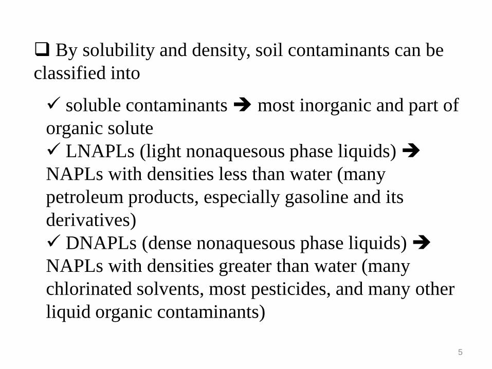
By solubility and density, soil contaminants can be classified into
soluble contaminants most inorganic and part of organic solute LNAPLs (light nonaquesous phase liquids) NAPLs with densities less than water (many petroleum products, especially gasoline and its derivatives) DNAPLs (dense nonaquesous phase liquids) NAPLs with densities greater than water (many chlorinated solvents, most pesticides, and many other liquid organic contaminants)
5
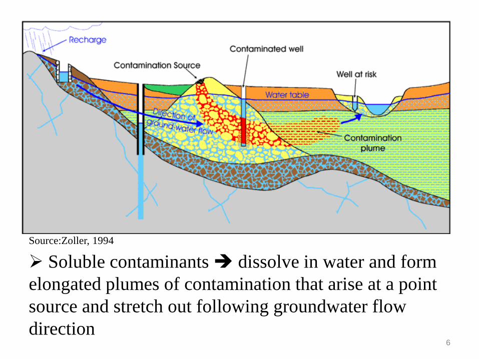
Soluble contaminants dissolve in water and form elongated plumes of contamination that arise at a point source and stretch out following groundwater flow direction
Source:Zoller, 1994
6
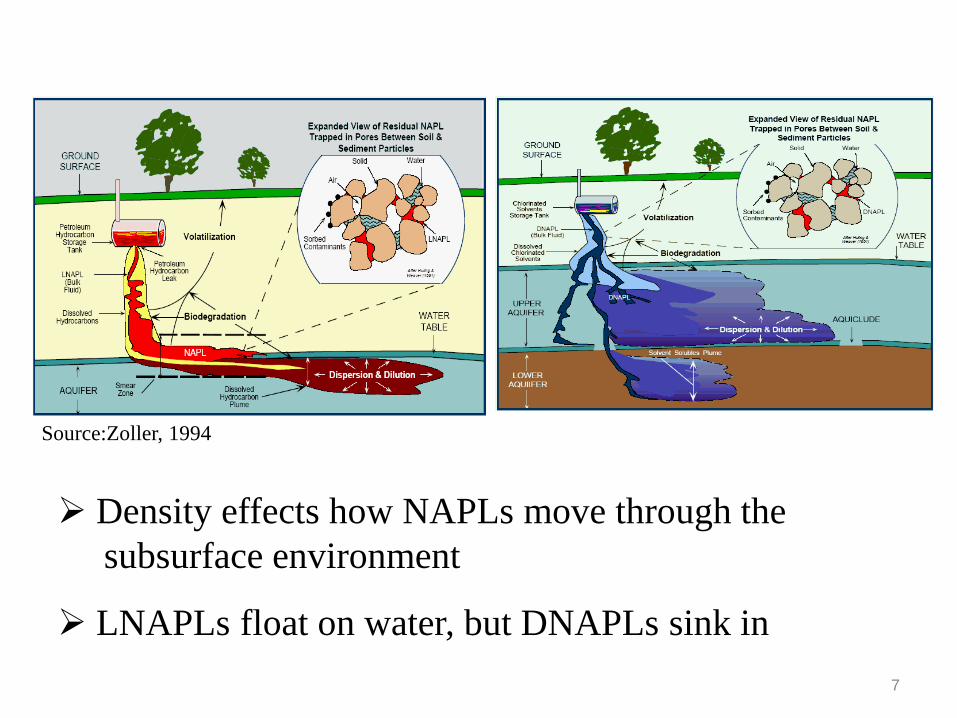
Density effects how NAPLs move through the subsurface environment LNAPLs float on water, but DNAPLs sink in
Source:Zoller, 1994
7

NAPLs slight-solubility of these contaminants is sufficient to produce plumes of dissolved constituents move off into the surrounding environment Serious groundwater pollution over relatively large volumes of aquifer arise from very small spills or leaching rates As long as NAPLs remains in the ground aqueous-phase continuous to be released creating long-term pollution (tens to hundreds of years)
Presence of NAPLs in subsurface One of the major environmental concerns
8
3.2.1 Lump parameters for contaminant quantification
3.2 Characteristics of soil contaminants
(1) Total petroleum hydrocarbons (TPH)
A remarkably wide array of compounds that originally come from crude oil (C1 to C40) So many different chemicals in crude oil and in other petroleum products it is not practical to measure each one separately measure the total amount of TPH at a site Chemicals that may be found in TPH hexane, jet fuels, mineral oils, BTEX, and naphthalene, as well as other petroleum products and gasoline components can be determined by GC analysis
9
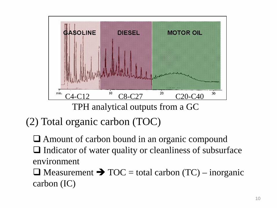
TPH analytical outputs from a GC (2) Total organic carbon (TOC) Amount of carbon bound in an organic compound Indicator of water quality or cleanliness of subsurface environment Measurement TOC = total carbon (TC) – inorganic carbon (IC)
10
C4-C12 C8-C27 C20-C40

(3) Biological oxygen demand (BOD)
A chemical procedure for determining the uptake rate of dissolved oxygen by the biological organisms in a sample Widely used parameter of organic pollution (e.g. investigation of remediation projects Measurement BOD5 and BODultimate
(4) Chemical oxygen demand (COD)
The mass of oxygen consumed per liter of sample solution Used to estimate the total oxygen demand of contaminated sites Approximately 65% of COD BOD
11
Relationships between BOD and COD
COD > BOD
Many organic substances which are difficult to oxidize biologically (e.g., lignin) can be oxidized chemically
Inorganic substances that are oxidized by the dichromate increase the apparent organic content of the sample high COD values may occur because of the presence of inorganic substances with which the dichromate can react
Certain organic substances may be toxic to the microorganisms used in the BOD test
12
BOD/COD ≥ 0.5 easily treated by biological means (biodegradable organics)
BOD/COD ≤ 0.3 have some toxic compounds or acclimated microorganisms may required in the stabilization (non-biodegradable organics)
(1) Solubility
The property of a solid, liquid, or gaseous chemical substance called solute to dissolve in a liquid solvent to form a homogeneous solution Measurement of the solubility of a pure substance in a specific solvent the saturation concentration where adding more solute does not increase the concentration of the solution (the solution is equilibrium with the substance at a specified temperature and pressure, e.g. 25 ºC, 1 atm)
3.2.2 Contaminant properties
13
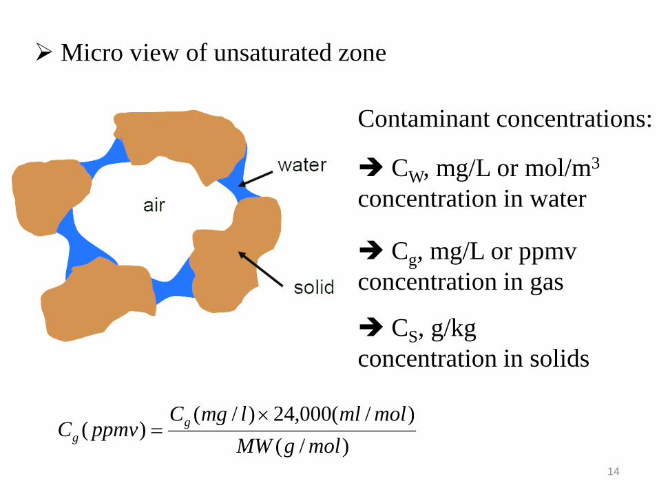
Micro view of unsaturated zone
Contaminant concentrations: CW, mg/L or mol/m3
concentration in water Cg, mg/L or ppmv concentration in gas CS, g/kg concentration in solids
)/()/(000,24)/(
)(molgMW
molmllmgCppmvC g
g
×=
14
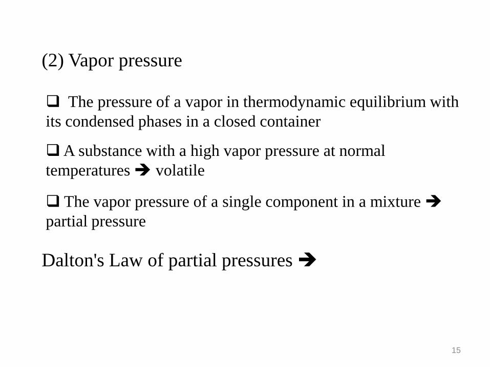
(2) Vapor pressure
The pressure of a vapor in thermodynamic equilibrium with its condensed phases in a closed container A substance with a high vapor pressure at normal temperatures volatile The vapor pressure of a single component in a mixture partial pressure
Dalton's Law of partial pressures
15

For a gas mixture containing nA mole of gas A, nB mole of gas B, and nC mole of gas C, with total volume = V and temperature = T
The partial pressures
totaltotal
AAA P
nn
VRTnP == total
total
BBB P
nn
VRTnP ==
totaltotal
CCC P
nn
VRTnP ==
16
"In a mixture of gases, each gas exerts pressure independently of the other gases. The partial pressure of each gas is proportional to the amount (as measured by percent volume of mole number) of that gas in the mixture"

The amount of a gas that will dissolve in a solution is directly proportional to the partial pressure of that gas in contact with the solvent.
(3) Henry’s law constant
Henry's Law
Linkage of solubility and vapor pressure gas-liquid transfer
KH = w
i
CP
Where Pi = partial pressure of a contaminant i in the gas (atm) CW = concentration of the contaminant i in the solution (mol/m3) KH = Henry's law constant (atm-m3/mol)
17

KH has dimensions (atm-m3/mol)
KHʹ dimensionless
RTKK H
H ='
Where R = gas constant = 8.20575 18×10-5 (atm-m3/mol-K) T = temperature (K)
Gas O2 H2 CO2 N2 KH (atm-m3/mol) 0.769 1.282 0.029 1.639 Gas He Ne Ar CO
KH (atm-m3/mol) 2.702 2.222 0.714 1.052
Henry's law and constants
18

(4) Interfacial tension with water A measurement of the cohesive (excess) energy present at an interface arising from the imbalance of forces between molecules at an interface (gas/liquid, liquid/liquid, gas/solid, liquid/solid) in units of dynes/cm Plays an important role in emulsification which is the process of preparing emulsions during some soil remediation treatments
19

3.3.1 Hydrodynamic Processes
3.3 Processes affecting subsurface materials and contaminants transport
(1) Advection
Refers to the movement caused by the flow of groundwater rate of advective contaminant migration equal to the rate of ground water flow
Advective flow velocities are calculated from Darcy's law
Darcy’s velocity (v), or discharge velocity v = Ki Seepage velocity (vS) since the actual flow is limited to the pore space only vS = v /ne = Ki/ne
20
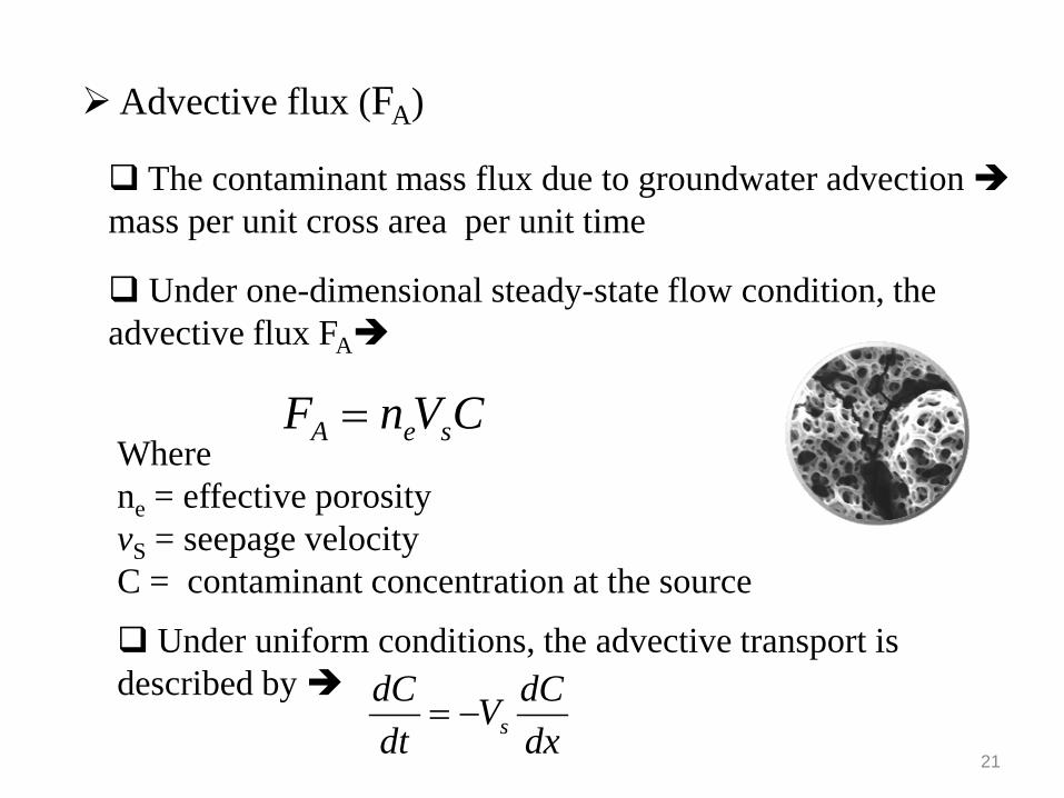
Advective flux (FA)
The contaminant mass flux due to groundwater advection mass per unit cross area per unit time
Under one-dimensional steady-state flow condition, the advective flux FA
CVnF seA =Where ne = effective porosity vS = seepage velocity C = contaminant concentration at the source
21 dxdCV
dtdC
s−=
Under uniform conditions, the advective transport is described by

(2) Dispersion
Spreading of the contaminant as it moves in a porous medium Two underlying processes molecular diffusion and mechanical dispersion
Hydrodynamic dispersion = molecular diffusion + mechanical dispersion
Molecular Diffusion spread due to concentration gradients without flow of water
22

Molecular diffusive flux (FD) Movement of contaminant mass in porous media by molecular diffusion (Brownian motion) – proportional to concentration gradient
dxdCnD
dxdCnDF eeD 0
* τ−=−=Where FD = diffusive mass flux per unit area per unit time D* = effective diffusion coefficient = τ D0
τ = tortuosity coefficient (<1) D0 = self-diffusion coefficient ne = effective porosity dC/dx = contaminant concentration gradient
Based on the Fick’s first law, the contaminant diffuse rate in soil is given by
2
2*
dxCdD
dtdC
=23

Example 3-1: At a landfill site, leachate acculmulated over a 0.3-m thick clay liner contains dissolved chloride in a concentration of 1000 mg/l. If the tortousity is equal to 0.5, what would be the concentration of chloride at a depth of 3m after 100 years of diffusion/ Neglect the effects of advection.
The contaminant concentration at a distance x from the source at time t (with an initial concentration of C0) is given by
)2
(),(*0tD
xerfcCtxC ×=
The complementary error function (erfc) is given by
ηπ
η deuerf
uerfuerfcu
∫ −=
−=
0
22)(
)(1)(
24
Presenter
Presentation Notes
P172 example 8.2

Mechanical Dispersion Occurs due to velocity variations of the flow in a porous media
Molecular diffusion is not a big factor in saturated groundwater flow mechanical dispersion dominates diffusion Molecular diffusion can be important (even dominant) in vapor transport in unsaturated (Vadose) zone
25
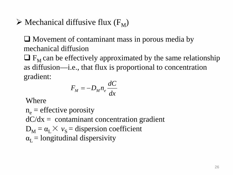
Mechanical diffusive flux (FM)
Movement of contaminant mass in porous media by mechanical diffusion FM can be effectively approximated by the same relationship as diffusion—i.e., that flux is proportional to concentration gradient:
dxdCnDF eMM −=
Where ne = effective porosity dC/dx = contaminant concentration gradient DM = αL× vS = dispersion coefficient αL = longitudinal dispersivity
26
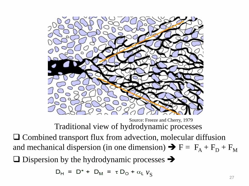
Source: Freeze and Cherry, 1979 Traditional view of hydrodynamic processes
Combined transport flux from advection, molecular diffusion and mechanical dispersion (in one dimension) F = FA + FD + FM
Dispersion by the hydrodynamic processes
27 vS

Application of the ADE (Advection-Dispersion Equation)
-- ADE is widely used in environmental problems dealing with transport of solutes in a mobile medium.
-- For example Oil tank leakage in a site: What is C in the well t years?
28

3.3.2 Abiotic Processes
Adsorption
a phenomenon by which chemicals become associated with solid phases
Adsorption chemicals adhere to surface of solid Absorption chemicals penetrate into solid Sorption includes both
29

If the adsorptive process is rapid compared with the flow velocity contaminant chemicals will reach an equilibrium condition adsorbed phase and the process can be described by an equilibrium adsorption isotherm Adsorption depends on properties of soil particles, chemistry of adsorbate, pH and temperature of water each application requires development of adsorption isotherm An adsorption isotherm relates S (solid phase concentration = mass of absorbate (contaminants)/ mass of adsorbent) to C (liquid phase concentration of absorbate) Adsorption process is quantified via an adsorption isotherm which can take multiple forms
30

The linear adsorption isotherm can be described by the equation: S = Kd C Where S = mass of contaminant adsorbed per dry unit weight of the solid adsorbent (mg/kg) C = concentration of contaminants in solution in equilibrium with the mass of contaminants adsorbed onto the solid adsorbent (mg/l) Kd = distribution coefficient (L/kg)
- We can develop a differential equation to describe the slope of a linear isotherm:
dKCC=
∂∂
Kd = slope of the linear adsorption isotherm
31
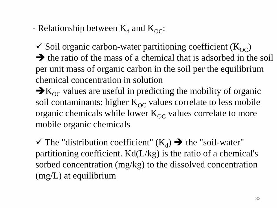
- Relationship between Kd and KOC:
Soil organic carbon-water partitioning coefficient (KOC) the ratio of the mass of a chemical that is adsorbed in the soil per unit mass of organic carbon in the soil per the equilibrium chemical concentration in solution KOC values are useful in predicting the mobility of organic soil contaminants; higher KOC values correlate to less mobile organic chemicals while lower KOC values correlate to more mobile organic chemicals
The "distribution coefficient" (Kd) the "soil-water" partitioning coefficient. Kd(L/kg) is the ratio of a chemical's sorbed concentration (mg/kg) to the dissolved concentration (mg/L) at equilibrium
32

KOC is the Kd normalized to total organic carbon content KOC is chemical- specific more applied to characterizing organic contaminants Kd is chemical- and site- specific more applied to characterizing heavy metals For organics, Kd may be calculated by multiplying KOC by foc (the mass fraction of soil organic carbon content Kd = KOC × fOC
Example:
33

- We can develop a term called the retardation factor, R, to describe linear adsorption:
dd KBθ
+= 1Rwhere Bd = bulk density of the soil (g/cm3) θ = volumetric moisture content (fraction) Kd = partition coefficient (L/kg)
- The governing equation is affected by this term as follows:
If vx = average linear groundwater flow velocity, then vC = velocity of the contaminant
Rxνν =c
34

Example 3-2: pesticide in aquifer (Springer, 1994) Sample
# Initial C (mg/L)
Equilibrium C (mg/L)
Mass adsorbed (mg/kg)
1 1 0.79 1.25 2 0.5 0.39 0.66 3 0.1 0.07 0.18 4 0.05 0.03 0.096 5 0.01 0.01 0.018 6 0.005 0.003 0.011 7 0 0 0
(1) Plot the data on a provided graph (2) Determine Kd. (3) Assume a bulk density of 1.78 g/cm3 and a volumetric moisture content of 0.45. Calculate the retardation factor. (4) If the average groundwater velocity is 50 cm/day, what is the velocity of the pesticide transport?
35
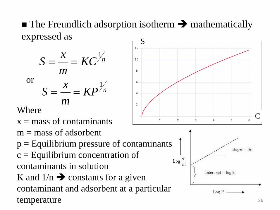
The Freundlich adsorption isotherm mathematically expressed as
Where x = mass of contaminants m = mass of adsorbent p = Equilibrium pressure of contaminants c = Equilibrium concentration of contaminants in solution K and 1/n constants for a given contaminant and adsorbent at a particular temperature
nKCmxS
1==
C
S
nKPmxS
1==
or
36
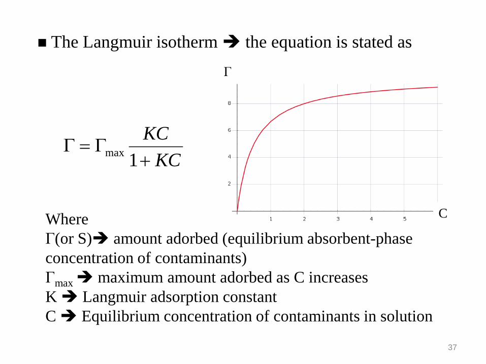
The Langmuir isotherm the equation is stated as
KCKC+
Γ=Γ1max
Г
C Where Г(or S) amount adorbed (equilibrium absorbent-phase concentration of contaminants) Гmax maximum amount adorbed as C increases K Langmuir adsorption constant C Equilibrium concentration of contaminants in solution
37

Linear isotherm Freundlich isotherm Langmuir isotherm
Гmax
38
Presenter
Presentation Notes
3.3.3 Biotic processes
Biochemical transformation (Biodegradation)
Microbial process that converse organic contaminants into water, CO2, inorganic materials and biomass The most important mechanism for removal of contaminant from the environment Organic molecules are transformed (degraded) by enzymes that reside within the cell walls of microorganisms
39
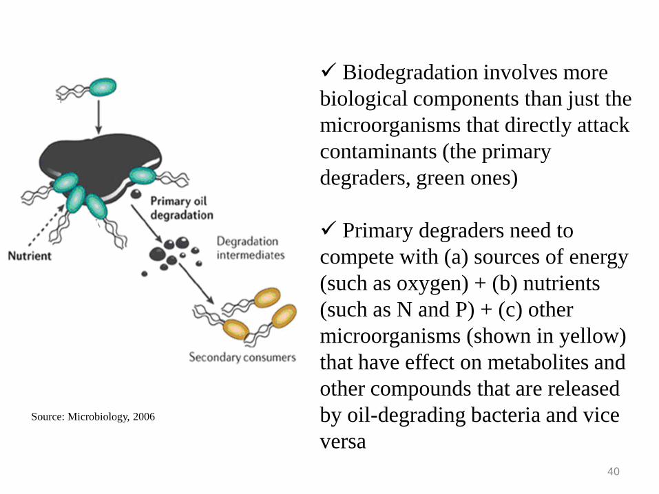
Source: Microbiology, 2006
Biodegradation involves more biological components than just the microorganisms that directly attack contaminants (the primary degraders, green ones)
Primary degraders need to compete with (a) sources of energy (such as oxygen) + (b) nutrients (such as N and P) + (c) other microorganisms (shown in yellow) that have effect on metabolites and other compounds that are released by oil-degrading bacteria and vice versa
40

=KH=
=Kd=
KH
Kd
3.4 Relationships of CW, Cg, and CS
41

Volume-related properties
42

Where…
Contaminants concentration in soil …
In the zone of aeration
In the zone of saturation 43

Example 3-3: During site investigations of a former gas station, a soil sample was collected in unsaturated silt at 2 meters below ground surface. The water table is located at 4 meters below ground surface. A laboratory analysis of the soil sample for TCE found a concentration of 1 mg/kg in this sample. The owner states he never used TCE on the site and the soil must have been contaminated by the underlying ground water, which is contaminated by a neighboring business. If the measured TCE concentration in the ground water is 10,000 μg/L, show mathematically if it is a reasonable hypothesis that the soil was contaminated by the underlying ground water. You can assume steady-state conditions, that the soil has a porosity of 0.4, that the soil saturation is 0.25, that the bulk density of the soil is 1.65 g/mL, and that the soil fraction organic carbon (fOC) is 0.001. The Henry’s Law constant for TCE is 9.1×10⁻³ atm-m3/mole You can also assume that there is only molecular diffusion within the vadose zone. 44