Lecture 3 - Aalborg Universitethomes.nano.aau.dk/lg/Lab-on-Chip2008_files/Lab-on-chip2008_3.pdf ·...
43
Lecture 3 Fluid Kinematics: Velocity field, Acceleration, Reynolds Transport Theorem and its application
Transcript of Lecture 3 - Aalborg Universitethomes.nano.aau.dk/lg/Lab-on-Chip2008_files/Lab-on-chip2008_3.pdf ·...

Lecture 3
Fluid Kinematics: Velocity field, Acceleration, Reynolds Transport
Theorem and its application

Aims
• Describing fluid flow as a field• How the flowing fluid interacts with the
environment (forces and energy)

Lecture plan
• Describing flow with the fields: Eulerian vs. Lagrangian description.
• Flow analysis: Streamlines, Streaklines, Pathlines.• How to perform calculations in the field description:
the Material Derivative• Reynold’s Transport Theorem• Application of Reynolds transport theorem:
Continuity, Momentum and Energy conservation
Velocity field
uv
dxdy
=
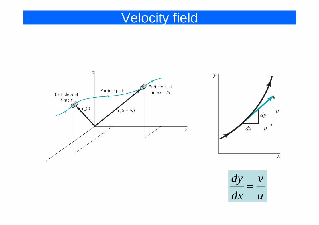
Velocity field: example
The calculated velocity field in a shipping channel is shown as the tide comes in and goes out. The fluid speed is given by the length and color of the arrows. The instantaneous flow direction is indicated by the direction that the velocity arrows point.
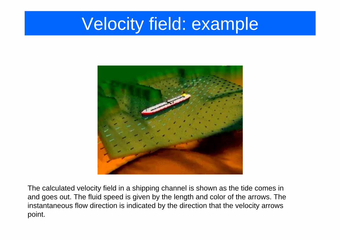
Velocity field is given by:
))(/( 0 jyixlvv −=• Sketch the field in the first quadrant• find where velocity will be equal to v0
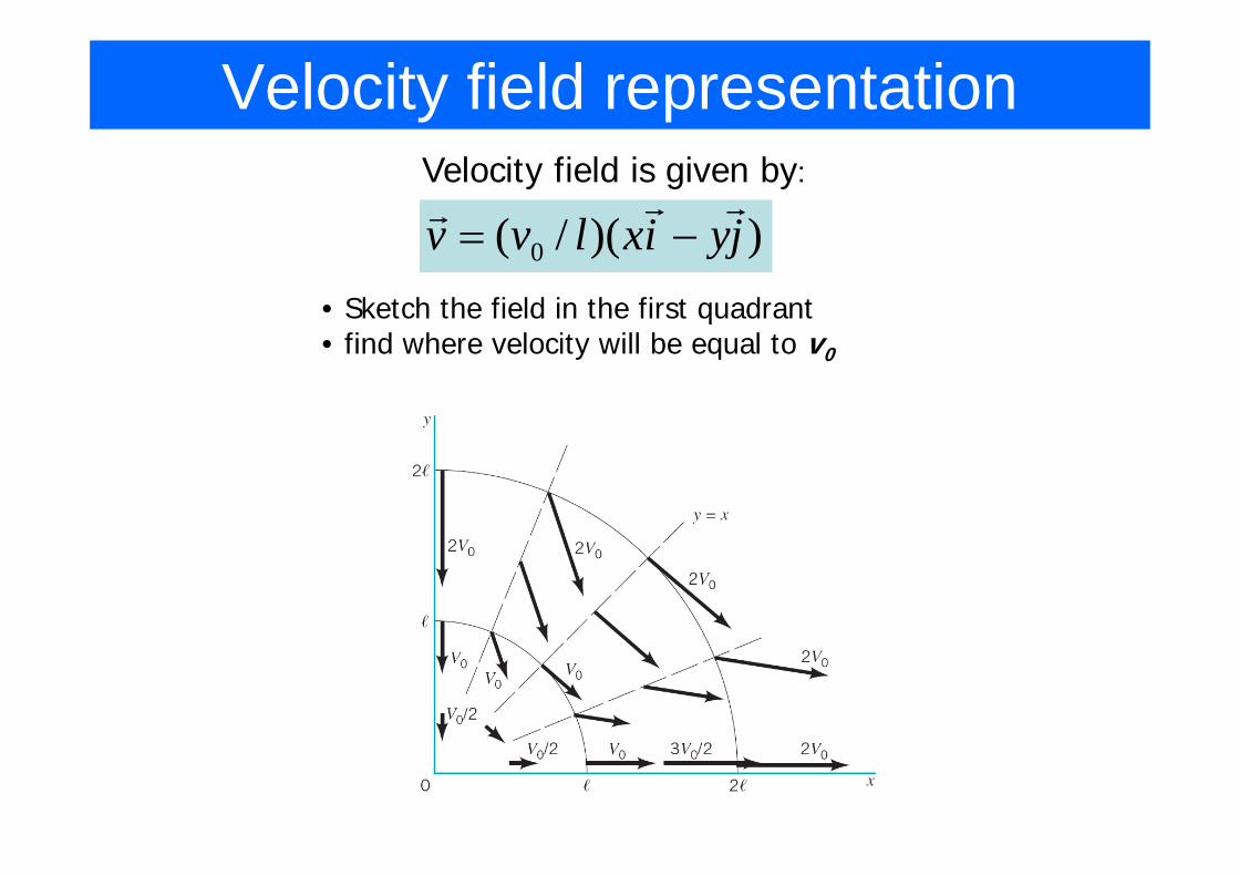
Velocity field representation

Eulerian and Lagrangian flow description
• Eulerian method – field concept is used, flow parameters (T, P, v etc.) are measured in every point in space vs. time
• Lagrangian method – an individual fluid particle is followed, parameters associated with this particle are followed in time
Example: Smoke coming out of a chimney

1D, 2D and 3D flow
Flow visualization of the complex three-dimensional flow past a model airfoil
The flow generated by an airplane is made visible by flying a model Airbus airplane through two plumes of smoke. The complex, unsteady, three-dimensional swirling motion generated at the wing tips (called trailing vorticies) is clearly visible

Flow types• Steady flow – the velocity at any given point in space doesn’t vary with
time. Otherwise the flow is called unsteady• Laminar flow – fluid particles follow well defined pathlines at any moment
in time, in turbulent flow pathlines are not defined.
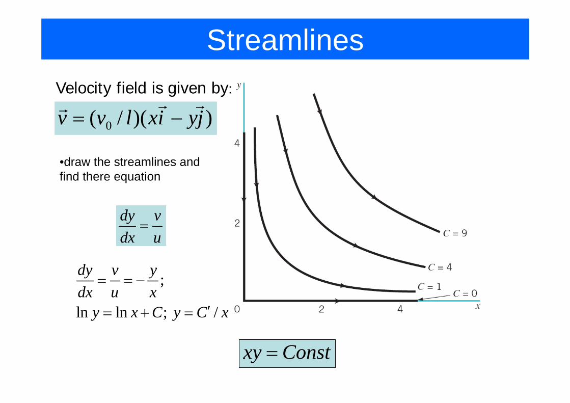
Constxy =
StreamlinesVelocity field is given by:
))(/( 0 jyixlvv −=
•draw the streamlines and find there equation
uv
dxdy
=
;
ln ln ; /
dy v ydx u x
y x C y C x
= = −
′= + =

Streamlines, Streaklines, Pathlines• Streamline – line that
everywhere tangent to velocity field
• Streakline – all particles that passed through a common point
• Pathline – line traced by a given particle as it flows
streamlines

Imaging flow in a microfluidic channel• Flow is seeded with fluorescent particles and imaged…
(Project 5th semester Fall 2006)
Flow through a loosely packed microspheres bed
Flow at a channel turn. Flow is disturbed by a microwire

Example
Water flowing from an oscillating slit:
jvivytuv 000 ))/(sin( +−= ω


Material derivative
• Particle velocity
),( trV AA
• Particle acceleration
tz
zV
ty
yV
tx
xV
tV
dtdVtra AAAAAAAA
AA ∂∂
∂∂
+∂∂
∂∂
+∂∂
∂∂
+∂∂
==),(
DtD
zw
yv
xu
ttr VVVVV
=∂∂
+∂∂
+∂∂
+∂∂
=),(a
• Material derivative )V ∇•+∂∂
=∂∂
+∂∂
+∂∂
+∂∂
= ( tz
wy
vx
utDt
D

Material derivative
• is the rate of changes for a given variable with time for a given particle of fluid.
)V ∇•+∂∂
=∂∂
+∂∂
+∂∂
+∂∂
= ( tz
wy
vx
utDt
D
Unsteadiness of the flow(local acceleration)
Convective effect(convective acceleration)

Example: acceleration
Velocity field is given by: ))(/( 0 jyixlvv −=
Find the acceleration and draw it on scheme

Example: acceleration

Control volume and system representation
• System – specific identifiable quantity of matter, that might interact with the surrounding but always contains the same mass
• Control volume – geometrical entity, a volume in space through which fluid may flow
Governing laws of fluid motion are stated in terms in system, but control volume approach is essential for practical applications

Control volume and system representation
• Extensive property: B=mb (e.g. m (b=1), mv (b=v), mv2/2 etc)
intensive property∫=sys
sys bdB Vρ
∫
∫
∂∂
=∂∂
∂∂
=∂
∂
cv
cv
sys
sys
bdtt
B
bdtt
B
V
V
ρ
ρ
0;0 <∂∂
=∂∂
=∂∂
=∂
∂∫∫cv
cv
sys
sys dtt
Bdtt
BVV ρρ
Control volume: example

The Reynolds Transport theorem (simplified)
IIICVSYSttCVSYSt
+−=+=
)(::δ
)()()()(
)()(
ttBttBttBttB
tBtB
IIIcvsys
cvsys
δδδδ +++−+=+
=
tttB
tttB
ttBttB
ttBttB IIIcvcvsyssys
δδ
δδ
δδ
δδ )()()()()()( +
++
−−+
=−+
outflowinflow
Let’s consider an extensive property B:

• For fixed control volume with one inlet, one outlet, velocity normal to inlet/outlet
outincvsys BBt
BDt
DB+−
∂∂
=
22221111 bVAbVAt
BDt
DB cvsys ρρ +−∂∂
=
• Can be easily generalized:
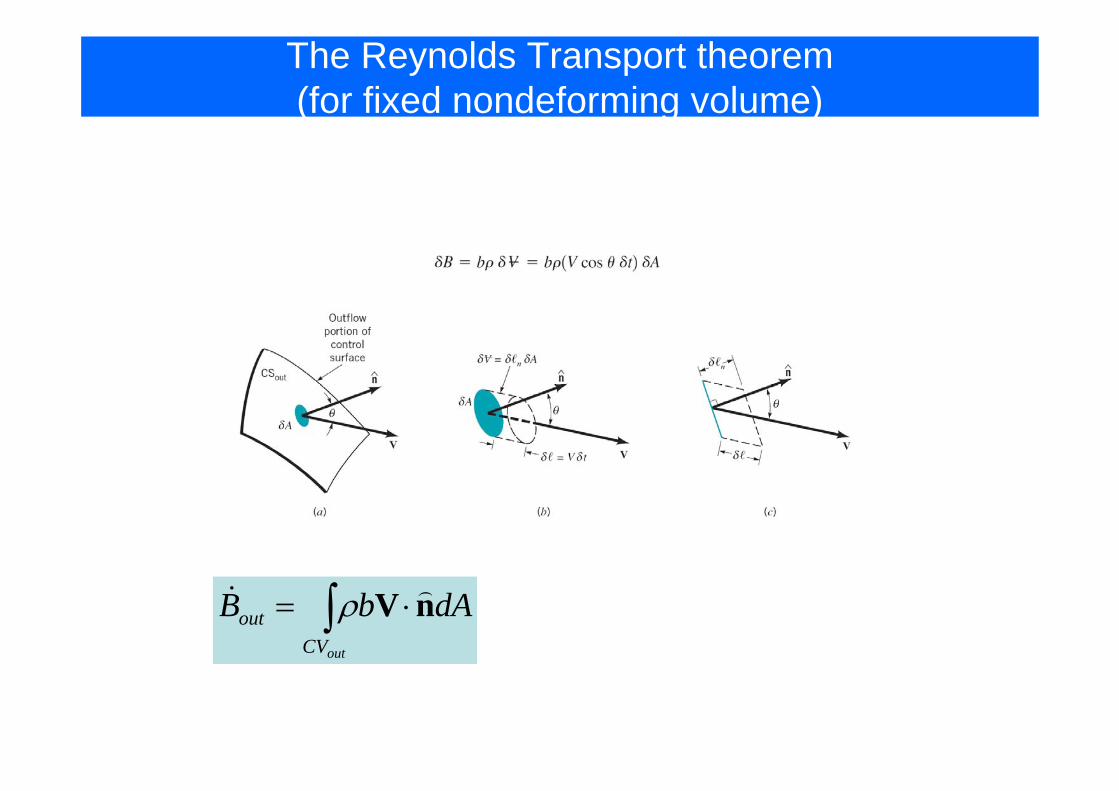
The Reynolds Transport theorem(for fixed nondeforming volume)
∫ ⋅=outCV
out dAbB nVρ

∫ ⋅+∂
∂=
CV
CVSys dAbt
BDt
DBnVρ
General Reynolds transport theorem for fixed control volume
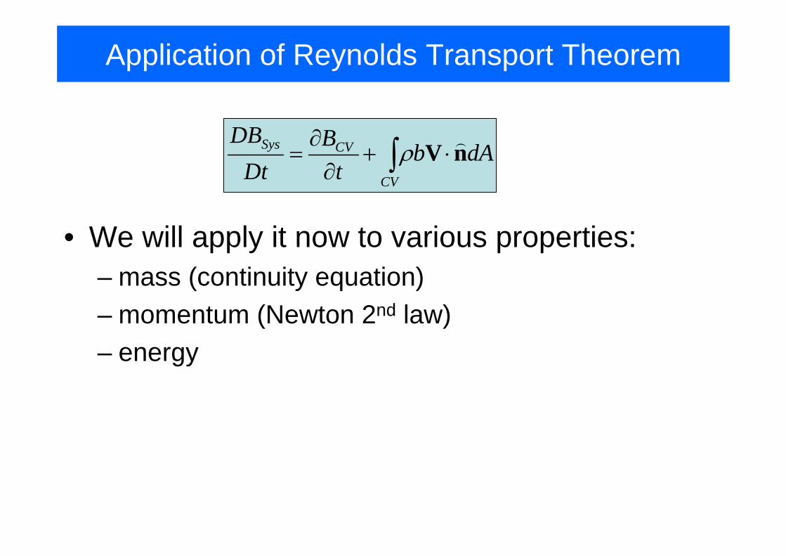
Application of Reynolds Transport Theorem
• We will apply it now to various properties:– mass (continuity equation)– momentum (Newton 2nd law)– energy
∫ ⋅+∂
∂=
CV
CVSys dAbt
BDt
DBnVρ

Conservation of mass
• The amount of mass in the system should be conserved:
0=⋅+∂∂
== ∫∫∫CVCVsys
Sys dAdt
dDtD
DtDM
nVρρρ VV
Continuity equation
m Q AVρ ρ= =
Mass flow rate through a section of control surface having area A:
Volume flow rate
A
V n dAV
A
ρ
ρ
⋅=∫
Average velocity:

• For incompressible flow, the volume flowrate into a control volume equals the volume flowrate out of it.
• The overflow drain holes in a sink must be large enough to accommodate the flowrate from the faucet if the drain hole at the bottom of the sink is closed. Since the elevation head for the flow through the overflow drain is not large, the velocity there is relatively small. Thus, the area of the overflow drain holes must be larger than the faucet outlet area

ExampleIncompressible laminar flow develops in a straight pipe of radius R. At section 1 velocity profile is uniform, at section 2 profile is axisymmetric and parabolic with maximum value umax. Find relation between U and umax, what is average velocity at section (2)?
2
1 1 2
2
1 max0
max
0
1 2 0
2
A
R
AU V n dA
rAU u rdrR
u U
ρ ρ
π
− + ⋅ =
⎡ ⎤⎛ ⎞− + − =⎢ ⎥⎜ ⎟⎝ ⎠⎢ ⎥⎣ ⎦
=
∫
∫

A jet of fluid deflected by an object puts a force on the object. This force is the result of the change of momentum of the fluid and can happen even though the speed (magnitude of velocity) remains constant.
Newton second law and conservation of momentum & momentum-of-momentum

Newton second law and conservation of momentum & momentum-of-momentum
∑∫ = syssys
FdDtD VρV
Rate of change of the momentum of the system
Sum of all external forces acting on the system
sys CV CS
D d d dADt t
ρ ρ ρ∂= + ⋅∂∫ ∫ ∫V V V V nV VOn the other hand:
In an inertial coordinate system:
At a moment when system coincide with control volume:sys contentsof
thecontrol volumeF F=∑ ∑
contentsofthecontrol volumeCV CS
d dA Ft
ρ ρ∂+ ⋅ =
∂ ∑∫ ∫V V V nV
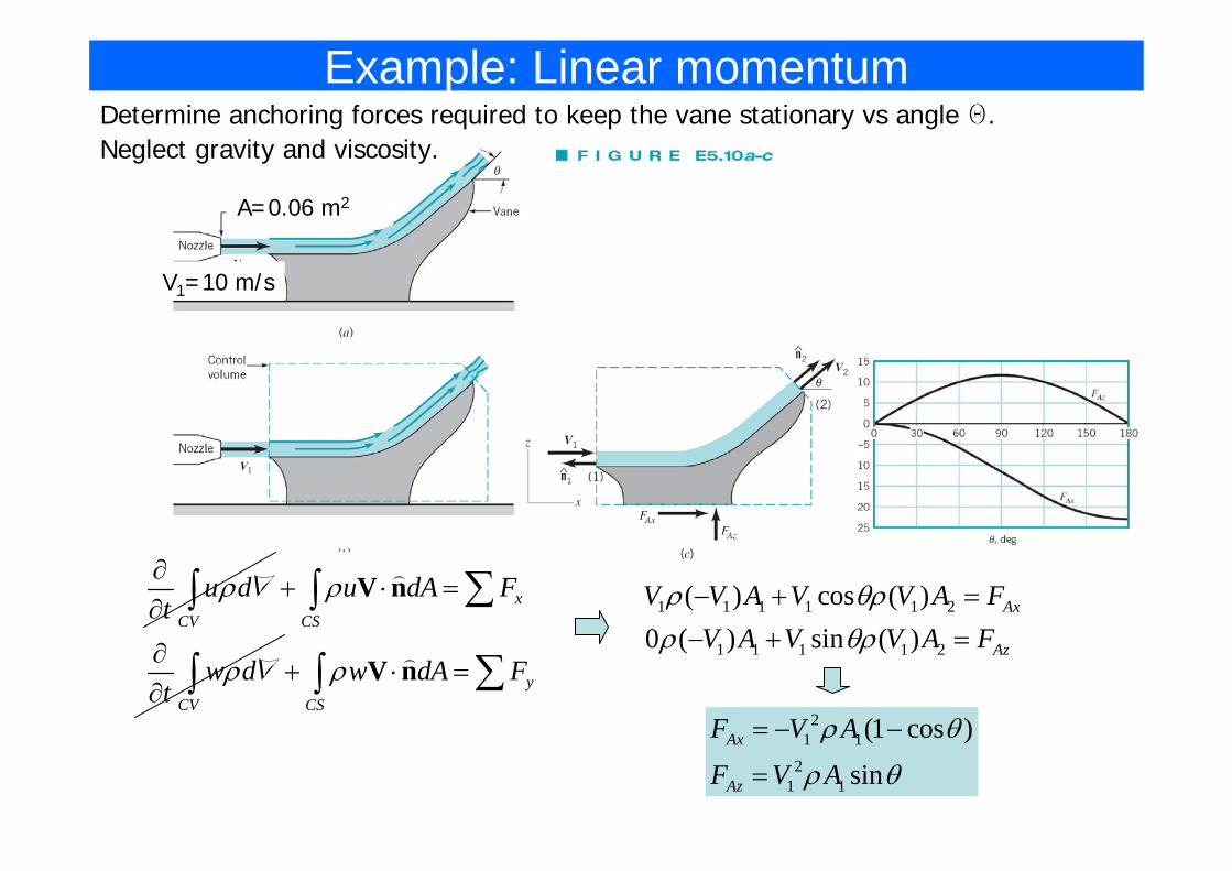
A=0.06 m2
V1=10 m/s
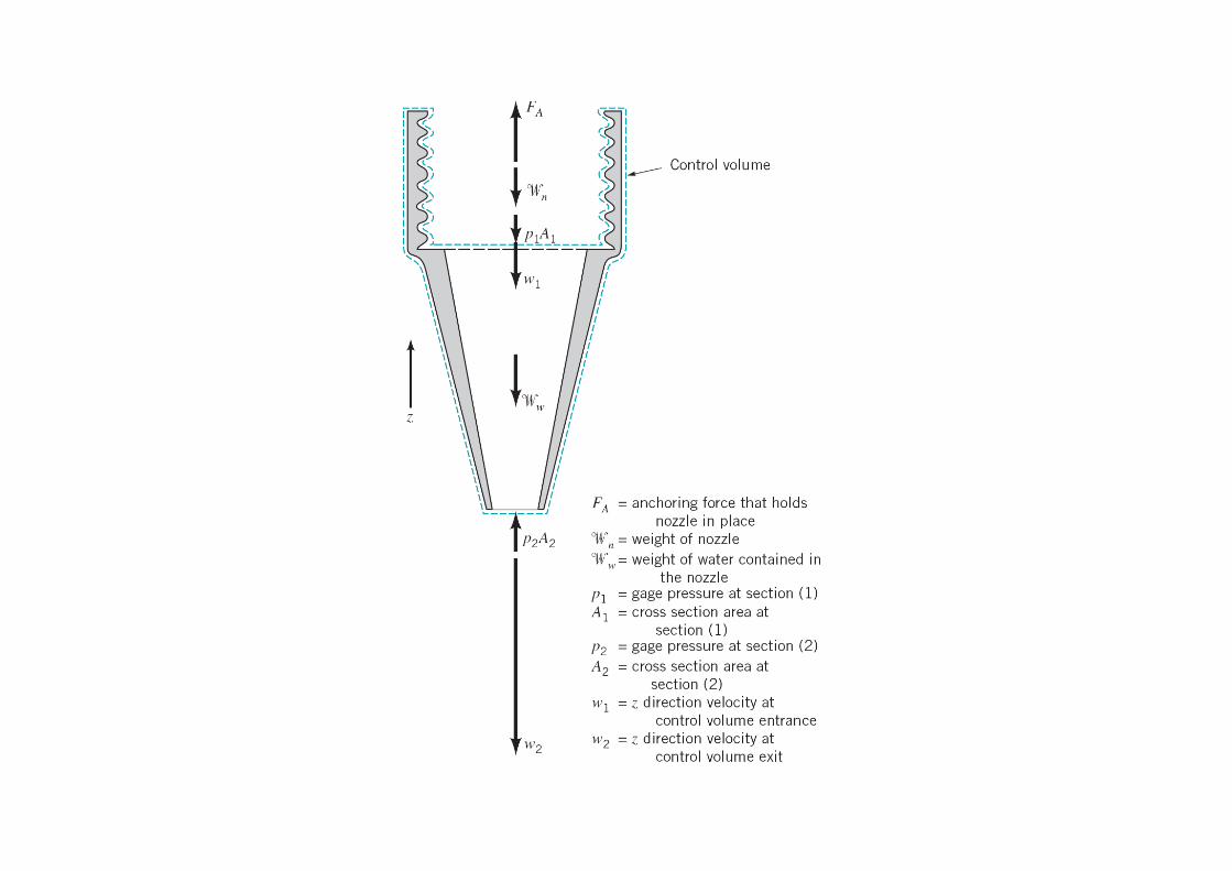
Example: Linear momentumDetermine anchoring forces required to keep the vane stationary vs angle Q. Neglect gravity and viscosity.
xCV CS
yCV CS
u d u dA Ft
w d w dA Ft
ρ ρ
ρ ρ
∂+ ⋅ =
∂
∂+ ⋅ =
∂
∑∫ ∫
∑∫ ∫
V n
V n
V
V
1 1 1 1 1 2
1 1 1 1 2
( ) cos ( )0 ( ) sin ( )
Ax
Az
V V A V V A FV A V V A F
ρ θρρ θρ
− + =
− + =
21 1
21 1
(1 cos )
sinAx
Az
F V A
F V A
ρ θ
ρ θ
= − −
=

Linear momentum: comments
• Linear momentum is a vector• As normal vector points outwards, momentum flow inside a
CV involves negative Vn product and moment flow outside of a CV involves a positive Vn product.
• The time rate of change of the linear momentum of the contents of a nondeforming CV is zero for steady flow
• Forces due to atmospheric pressure on the CV may need to be considered

Moment-of-Momentum Equation
The net rate of flow of moment-of-momentum through a control surface equals the net torque acting on the contents of the control volume.Water enters the rotating arm of a lawn sprinkler along the axis of rotation with no angular momentum about the axis. Thus, with negligible frictional torque on the rotating arm, the absolute velocity of the water exiting at the end of the arm must be in the radial direction (i.e., with zero angular momentum also). Since the sprinkler arms are angled "backwards", the arms must therefore rotate so that the circumferential velocity of the exit nozzle (radius times angular velocity) equals the oppositely directed circumferential water velocity.

The Energy Equation
Rate of increase of the total stored energy of the system
Net rate of energy addition by heat transfer into the system
Net rate of energy addition by work transfer into the system
syssys
WQdeDtD )( +=∫ Vρ
gzVue ++=2
2
Total stored energy per unit mass:

∫∫∫ ⋅+∂∂
=CSCVsys
dAedet
deDtD nVρρρ VV
Rate of increase of the total stored energy of the system
rate of increase of the total stored energy of the control volume
Net rate of energy flow out of the control volume
( )net net cvin inCV CS
e d e dA Q Wt
ρ ρ∂+ ⋅ = +
∂ ∫ ∫ V nV

Application of energy equation• Product V·n is non-zero only where liquid crosses the CS; if
we have only one stream entering and leaving control volume:
2 2 2
2 2 2out inCS out in
p V p V p Vu gz dA u gz m u gz mρρ ρ ρ
⎛ ⎞ ⎛ ⎞ ⎛ ⎞+ + + ⋅ = + + + − + + +⎜ ⎟ ⎜ ⎟ ⎜ ⎟
⎝ ⎠ ⎝ ⎠ ⎝ ⎠∫ V n
• If no shaft power is applied and we assume flow steady
2 2
( ),2 2
netinout out in in
out in out in net netin in
Qp V p Vgz gz u u q q
mρ ρ+ + = + + − − − =
lossavailable energy

Energy transfer
Work must be done on the device shown to turn it over because the system gains potential energy as the heavy (dark) liquid is raised above the light (clear) liquid. This potential energy is converted into kinetic energy which is either dissipated due to friction as the fluid flows down the ramp or is converted into power by the turbine and then dissipated by friction. The fluid finally becomes stationary again. The initial work done in turning it over eventually results in a very slight increase in the system temperature

Second law of thermodynamics
• Let’s apply “stream line energy equation” to an infinitesimally thin volume
dU TdS pdV= −
2
2 netin
p Vm du d d gdz Qδρ
⎡ ⎤⎛ ⎞⎛ ⎞+ + + =⎢ ⎥⎜ ⎟⎜ ⎟
⎝ ⎠ ⎝ ⎠⎣ ⎦
2
( )2 net
in
dp Vd gdz Tds qδρ
⎡ ⎤⎛ ⎞+ + = − −⎢ ⎥⎜ ⎟
⎝ ⎠⎣ ⎦
1( )du Tds pdρ
= −
For closed system in the absence of additional work:
0dqdST
− ≥If we take into account Clausius inequality: 2
02
dp Vd gdzρ
⎡ ⎤⎛ ⎞− + + ≥⎢ ⎥⎜ ⎟
⎝ ⎠⎣ ⎦

Application of energy equation• We can make the energy equation more concrete by noting:
– Work is usually transferred into liquid by rotating shaft:
shaft shaftT ωW =– Or by normal stress acting on a free surface
CS
ˆ ˆ
ˆnormal stress
normal stress
A p A
p dA
δ σ δ δ⋅ − ⋅
− ⋅∫W = n V = V n
W = V n
• The energy equation is now:
2
( )2 net shaft cv
in inCV CS
p Ve d u gz dA Q Wt
ρ ρρ
⎛ ⎞∂+ + + + ⋅ = +⎜ ⎟∂ ⎝ ⎠
∫ ∫ V nV

Example: Efficiency of a fan

Problem 4.20
• Determine local acceleration at points 1 and 2. Is the average convective acceleration between these points negative, zero or positive?

Problems
• 5.102 Water flows steadily down the inclined pump. Determine: – The pressure difference, p1-p2;– The loss between sections 1 and 2– The axial force exerted on the pipe
by water
• 4.20. Determine local acceleration at points 1 and 2. Is the average convective acceleration between these points negative, zero or positive?