Lecture 24: Query Execution

Monday, November 20, 2000

Outline

• Finish sorting based algorithms (6.5)

• Two pass algorithms based on hashing (6.6)

• Two pass algorithms based on indexes (6.7)

Cost Parameters

Recall:

• B(R) = number of blocks for relation R

• T(R) = number of tuples in relation R

• V(R, a) = number of distinct values of attribute a

Two-Pass Algorithms Based on Sorting

• Recall: multi-way merge sort needs only two passes !

• Assumption: B(R) <= M2

• Cost for sorting: 3B(R)

Two-Pass Algorithms Based on Sorting

Duplicate elimination (R)• Trivial idea: sort first, then eliminate duplicates• Step 1: sort chunks of size M, write

– cost 2B(R)

• Step 2: merge M-1 runs, but include each tuple only once– cost B(R)

• Total cost: 3B(R), Assumption: B(R) <= M2

Two-Pass Algorithms Based on Sorting

Grouping: city, sum(price) (R)

• Same as before: sort, then compute the sum(price) for each group

• As before: compute sum(price) during the merge phase.

• Total cost: 3B(R)

• Assumption: B(R) <= M2

Two-Pass Algorithms Based on Sorting

Binary operations: R ∩ S, R U S, R – S• Idea: sort R, sort S, then do the right thing• A closer look:

– Step 1: split R into runs of size M, then split S into runs of size M. Cost: 2B(R) + 2B(S)

– Step 2: merge M/2 runs from R; merge M/2 runs from S; ouput a tuple on a case by cases basis

• Total cost: 3B(R)+3B(S)• Assumption: B(R)+B(S)<= M2

Two-Pass Algorithms Based on Sorting

Join R S• Start by sorting both R and S on the join attribute:

– Cost: 4B(R)+4B(S) (because need to write to disk)

• Read both relations in sorted order, match tuples– Cost: B(R)+B(S)

• Difficulty: many tuples in R may match many in S– If at least one set of tuples fits in M, we are OK– Otherwise need nested loop, higher cost

• Total cost: 5B(R)+5B(S)• Assumption: B(R) <= M2, B(S) <= M2

Two-Pass Algorithms Based on Sorting

Join R S

• If the number of tuples in R matching those in S is small (or vice versa) we can compute the join during the merge phase

• Total cost: 3B(R)+3B(S)

• Assumption: B(R) + B(S) <= M2

Two Pass Algorithms Based on Hashing

• Idea: partition a relation R into buckets, on disk• Each bucket has size approx. B(R)/M

• Does each bucket fit in main memory ?– Yes if B(R)/M <= M, i.e. B(R) <= M2

M main memory buffers DiskDisk

Relation ROUTPUT

2INPUT

1

hashfunction

h M-1

Partitions

1

2

M-1

. . .

1

2

B(R)

Hash Based Algorithms for

• Recall: (R) duplicate elimination

• Step 1. Partition R into buckets

• Step 2. Apply to each bucket (may read in main memory)

• Cost: 3B(R)

• Assumption:B(R) <= M2

Hash Based Algorithms for

• Recall: (R) grouping and aggregation

• Step 1. Partition R into buckets

• Step 2. Apply to each bucket (may read in main memory)

• Cost: 3B(R)

• Assumption:B(R) <= M2

Hash-based Join

• R S

• Recall the main memory hash-based join:– Scan S, build buckets in main memory– Then scan R and join

Partitioned Hash Join

R S• Step 1:

– Hash S into M buckets– send all buckets to disk

• Step 2– Hash R into M buckets– Send all buckets to disk

• Step 3– Join every pair of buckets

Hash-Join• Partition both relations

using hash fn h: R tuples in partition i will only match S tuples in partition i.

Read in a partition of R, hash it using h2 (<> h!). Scan matching partition of S, search for matches.

Partitionsof R & S

Input bufferfor Ri

Hash table for partitionSi ( < M-1 pages)

B main memory buffersDisk

Output buffer

Disk

Join Result

hashfnh2

h2

B main memory buffers DiskDisk

Original Relation OUTPUT

2INPUT

1

hashfunction

h M-1

Partitions

1

2

M-1

. . .

Partitioned Hash Join

• Cost: 3B(R) + 3B(S)

• Assumption: min(B(R), B(S)) <= M2

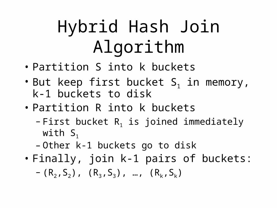
Hybrid Hash Join Algorithm

• Partition S into k buckets• But keep first bucket S1 in memory, k-1

buckets to disk• Partition R into k buckets

– First bucket R1 is joined immediately with S1 – Other k-1 buckets go to disk

• Finally, join k-1 pairs of buckets:– (R2,S2), (R3,S3), …, (Rk,Sk)

Hybrid Join Algorithm

• How big should we choose k ?

• Average bucket size for S is B(S)/k

• Need to fit B(S)/k + (k-1) blocks in memory– B(S)/k + (k-1) <= M– k slightly smaller than B(S)/M

Hybrid Join Algorithm

• How many I/Os ?• Recall: cost of partitioned hash join:

– 3B(R) + 3B(S)

• Now we save 2 disk operations for one bucket• Recall there are k buckets• Hence we save 2/k(B(R) + B(S))• Cost: (3-2/k)(B(R) + B(S)) =

(3-2M/B(S))(B(R) + B(S))

Indexed Based Algorithms

• Recall that in a clustered index all tuples with the same value of the key are clustered on as few blocks as possible

• Note: book uses another term: “clustering index”. Difference is minor…

a a a a a a a a a a

Index Based Selection

• Selection on equality: a=v(R)

• Clustered index on a: cost B(R)/V(R,a)

• Unclustered index on a: cost T(R)/V(R,a)

Index Based Selection

• Example: B(R) = 2000, T(R) = 100,000, V(R, a) = 20, compute the cost of a=v(R)

• Cost of table scan:– If R is clustered: B(R) = 2000 I/Os– If R is unclustered: T(R) = 100,000 I/Os

• Cost of index based selection:– If index is clustered: B(R)/V(R,a) = 100– If index is unclustered: T(R)/V(R,a) = 5000

• Notice: when V(R,a) is small, then unclustered index is useless

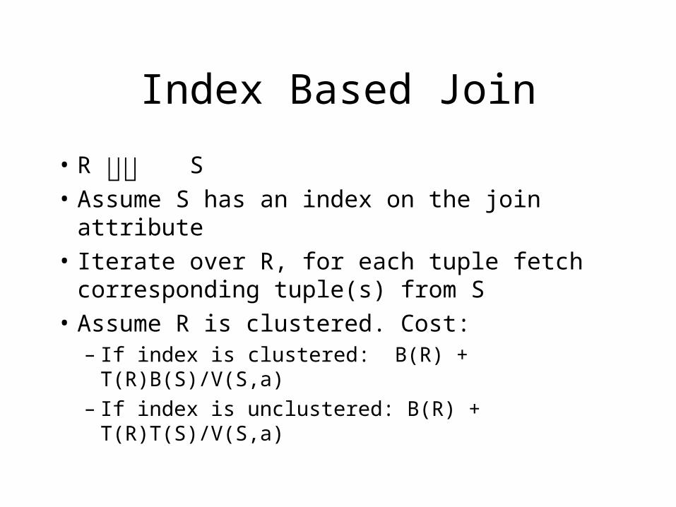
Index Based Join

• R S

• Assume S has an index on the join attribute

• Iterate over R, for each tuple fetch corresponding tuple(s) from S

• Assume R is clustered. Cost:– If index is clustered: B(R) + T(R)B(S)/V(S,a)– If index is unclustered: B(R) + T(R)T(S)/V(S,a)

Index Based Join

• Assume both R and S have a sorted index (B+ tree) on the join attribute

• Then perform a merge join (called zig-zag join)

• Cost: B(R) + B(S)