1

Lecture 2: International Real Business Cycle Models

Part1: Quantity Puzzle

a) Motivation

Issue: We now expand our study beyond consumption and the current account, to study a wider range of macroeconomic variables. We will learn about the literature studying business cycles in an international context.

Questions: - How much do national business cycles move together?

- Is this due more to similar shocks, or due to spillovers?

- Through what markets are shocks transmitted?

2

Methodology: - We here will use the approach of Real Business Cycle

(RBC) models. We start with Backus, et al (1992 JPE) which set the agenda for the resulting literature.

- This differs from models we’ve used in previous lectures, in

that output no longer is an exogenous endowment, but now is produced using capital and labor inputs.

- The vast majority of papers in this literature use two-country

models. This is different from the models considered so far in class,

which were small-open economy models.

3

b) Stylized facts:

Introduction:

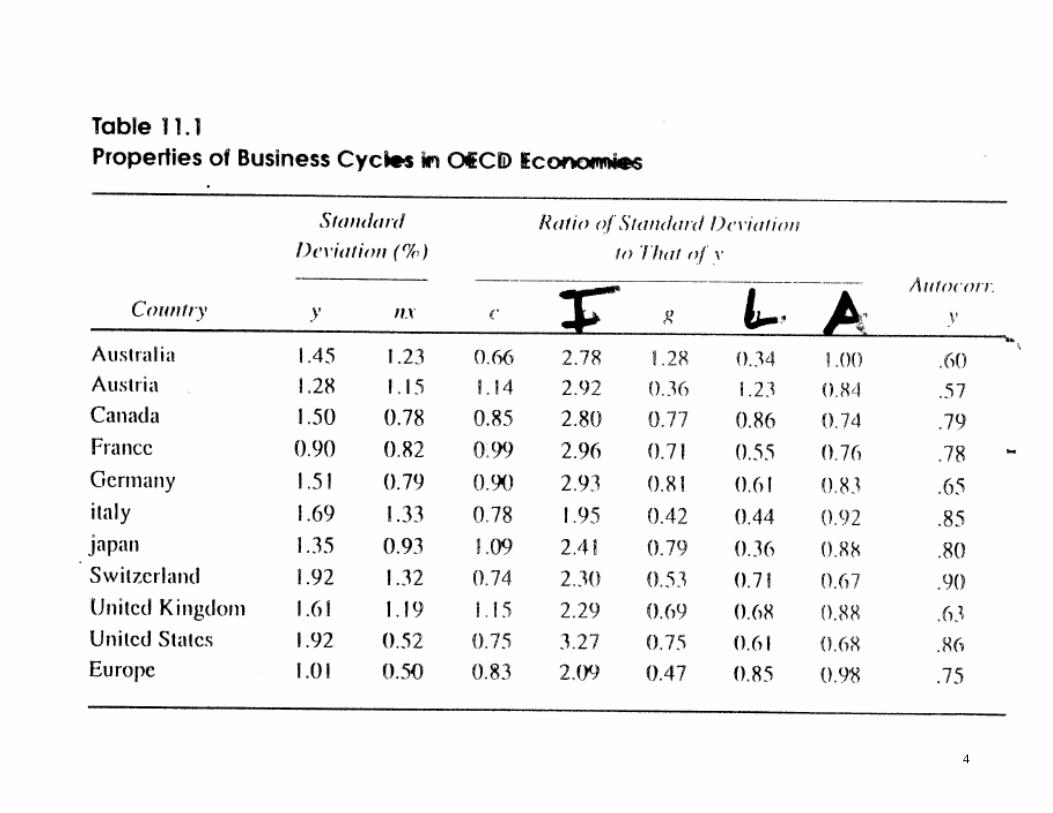
- Tables 11.1 and 11.2 from book chapter by Backus, et al.

- Data: 10 industrial countries and an aggregate of Europe, quarterly (1970:1 – 1990:2), and Hodrick-Prescott (HP) filtered to focus on business-cycle frequencies in data.

- Collect observations on the following: - Volatility: standard deviation

- Persistence: autocorrelation - Comovement: correlations

4

5

6

7

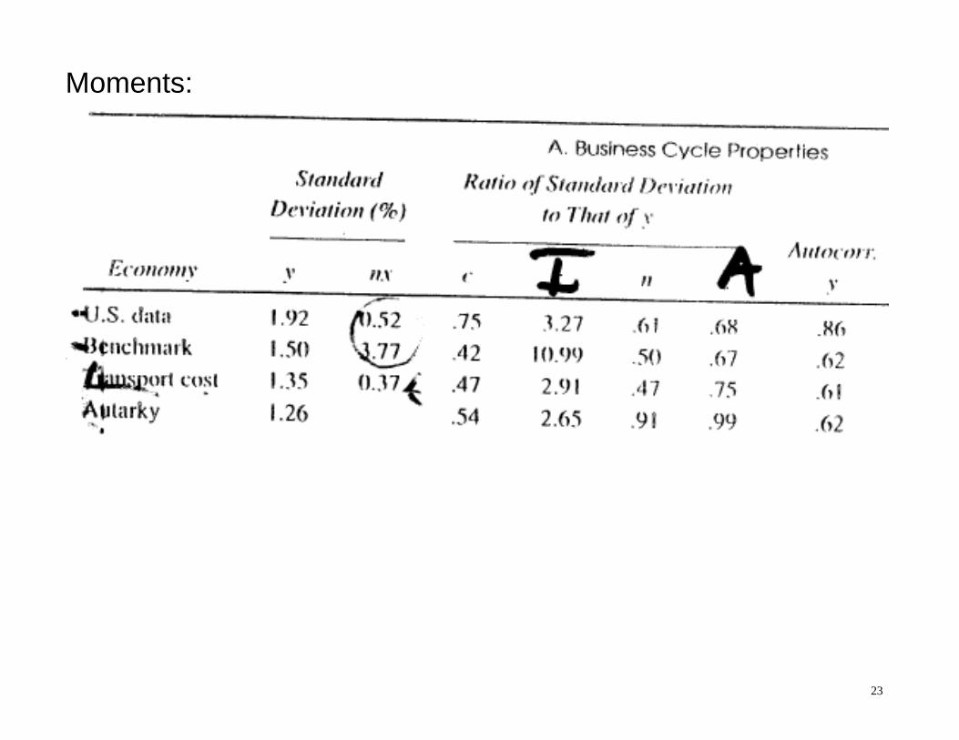
Table 11-1 Domestic Volatilities:

- Consumption is less volatile than output, reflecting consumption-smoothing.

- Investment is more volatile than output: 2-3 times.

- Countries differ much: output is more volatile in the US (sdev = 1.92); least in France (0.9).

Employment is procyclical

- The Solow residual is strongly procyclical, but less volatile than output.

- Technology shocks help explain fluctuations in output, but they need endogenous fluctuations in labor supply to amplify their effects on output.

8

Net exports:

- The trade balance is countercyclical in all 10 countries This is due to the volatile cyclical movement of investment,

which you will show in homework assignment. - This is contrary to the simple PV model of the CA we

studied where investment was exogenous. (Temporary rise in output should lead to a CA surplus.)

- Can be explained by allowing investment to rise in response

to output by large amount. (Will see this in homework assignment.)

Persistence: Output quite persistent, autocorr from 0.5 - 0.9.

9

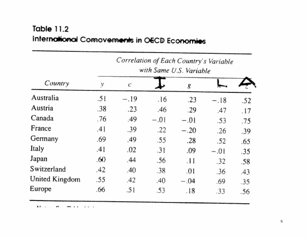
Table 11-2: International correlations: (with U.S.)

cor(Y,Y*) > cor (C,C*) for all cases

This is referred to as the Consumption Correlation Puzzle: Reasons this fact is puzzling:

- If asset markets pool consumption risk, then consumption should move similarly across countries.

- True even in a simple PV model of the CA with non-contingent bonds if think in a two-country context:

- A fall in home country endowment leads to a smaller fall in consumption because borrow from abroad.

- Foreign lenders cut their consumption in response to rise in real interest rate.

10

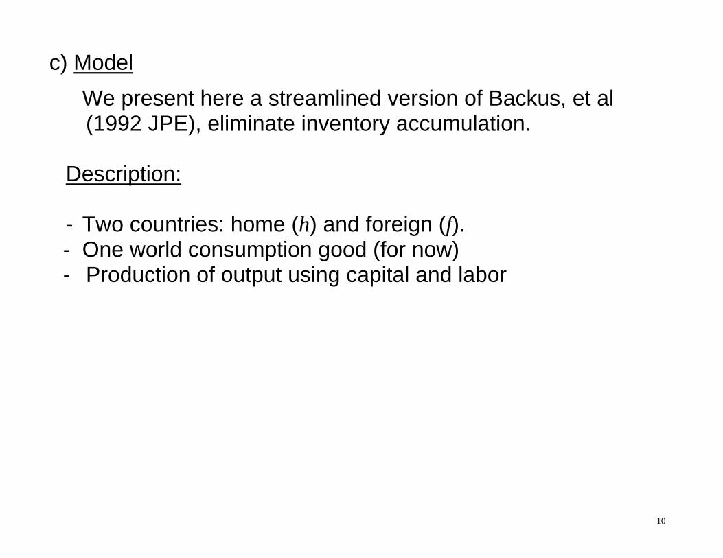
c) Model

We present here a streamlined version of Backus, et al (1992 JPE), eliminate inventory accumulation.

Description:

- Two countries: home (h) and foreign (f). - One world consumption good (for now) - Production of output using capital and labor

11

Preferences: Utility of representative household: cares about both

consumption ( C) and leisure (1-L), where L is labor.

fhiLCU ititit ,)1(111

Agent allocates one unit of time between work and leisure.

12

Production Production a function of labor (L) and capital (K) and

productivity term A: fhiLKALKFY itititititit ,, 1

Since both countries produce the same good, the resource

constraint is:

fthtfthtfthtftht GGIICCYY

13

Capital formation uses time-to-build structure. Additions to the stock of fixed capital require inputs of the

produced good for 4 periods:

ttt sKK 11 )1(

(For the home country; analogous for foreign. Skipped i subscripts on everything to avoid confusion)

Where t

js is the number of investment projects at date t that are j periods from completion.

tj

tj ss 1

1

It takes 4 periods for a capital good to be built and increase

the capital stock. So put in 1/4 of value added each period: If add up all the investment expenditure made in a period on

the projects at various stages of completion, it equals:

4

1 41

j

jtt sI

14

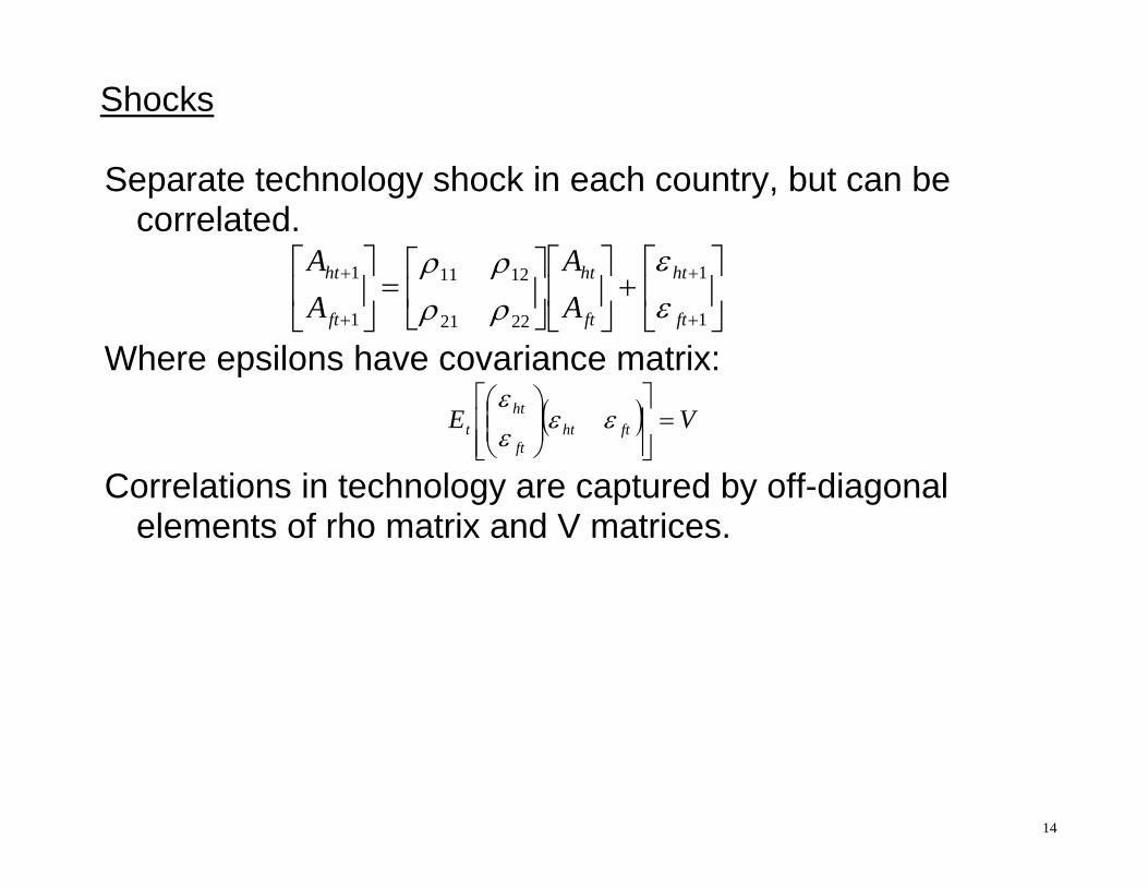
Shocks Separate technology shock in each country, but can be

correlated.

1

1

2221

1211

1

1

ft

ht

ft

ht

ft

ht

AA

AA

Where epsilons have covariance matrix:

VE ftht

ft

htt

Correlations in technology are captured by off-diagonal

elements of rho matrix and V matrices.

15

Equilibrium:

- We will assume that financial markets are complete. People in either country have access to a full set of conditional assets they can buy to insure against shocks.

- We could try to model explicitly all the assets and find the solution for the competitive equilibrium: see notes further below.

- Under complete markets, solution will be Pareto optimum.

- So we can also solve for the equilibrium as a single optimization problem of a social planner that maximizes the weighted sum of utilities of the two countries.

- So solve following subject to the constraints above:

0

max , 1 1 , 1tt ht ht ft ft

t

E U C L U C L

16

- Combining FOC for consumption with that for labor). ,

,,

''

'h

h

h

L tL t

C t

UF

U

equating marginal utility of lost leisure to marginal utility of extra consumption if provide additional labor.

- Combining FOC for home and foreign consumptions):

, ,1' '

h fC t C tU U

International Risk sharing condition, equating changes in marginal utility across countries.

17

Solution:

- Combine these optimality conditions with the resource constraints.

- Solve for a deterministic steady state (dropping uncertainty)

- Take a log-Linear approximation around the steady state. - Solve the linear system of equations, such as by method of

Blanchard and Kahn (1980): find unstable roots of system by eigen values; imposing the associated eigenvectors.

18

- Calibration:

o discount factor = 0.99 (assume quarterly period). o Intertemporal elasticity equals 0.5. o Technology shocks have persistence 0.9, and cross

persistence of 0.09. Correlation of epsilons are 0.258. - Simulate: 20 runs of 100 periods each. - Hodrick-Prescott (HP) filter and compute same statistics as

for actual data from the real economy. - Compare the moments from simulated data to those from

actual data.

19

d) Results: Consider a 1 % rise in A (positive epsilon for one period) in home country.

20

First do impulse responses: Home: - Rise in productivity raises output. - Also raises investment because of marginal productivity of

capital. Investment is very volatile in an open economy since it easy to borrow from abroad to finance investment.

- This makes net exports go negative (not shown explicitly,

but is apparent). - Also raises consumption as smoothed.

21

Foreign response:

22

Foreign: - Foreign investment moves the opposite way because want

to shift resources to where are the most productive. As a result output moves opposite as well. Falls at first.

- But consumption moves very similarly. Even though output

falls, consumption rises like in home country. - This is due to social planner / risk sharing.

23

Moments:

24

25

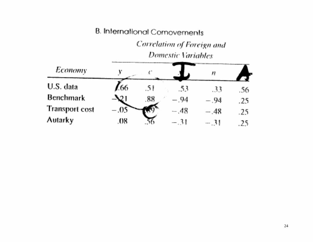
Correlations:

- Also see in correlations: output correlation is less than in data (-0.21 versus 0.66), but consumption correlation is higher than in data (.88 versus .51).

- Otherwise match things pretty well. (Investment a bit too volatile)

- Main problem is consumption correlation puzzle: consumption is less correlated in data than is output. Model says the opposite.

26

One Possible solution: Transport costs: - Try a version of model with costs of trading goods. - In a world budget constraint, impose a cost that is a

quadratic function of net exports. So if try to import goods to raise investment, becomes expensive.

hthththtt

tfthtfthtfthtftht

GICYnxwhere

nxGGIICCYY

2

- Mechanically, just add this term on to budget constraint

before do first order conditions. Calibrate, so on average cost is only about 1%.

- Result: lower response of net exports, and thereby

investment response to technology shock. But not affect consumption or output correlation much. Output cor rise from -.21 to -.05. Consumption cor rise from 0.88 to 0.89.

27

e) One explanation: Kollmann (JEDC 1996)

- Consider two-country RBC model like above, but replace complete asset market with one-period non-contingent bond (as in our simple intertemporal models earlier.

- It does not help in insuring against unforeseen shocks, but recall that it permits borrowing to smooth effects of shocks.

- If a temporary negative home technology shock lowers output, country can borrow abroad to boost consumption.

- Since a large country, the borrowing raises world interest rate, inducing foreign country to lower consumption, lend.

- So consumption falls in the foreign country, and this helps offset part of the fall in consumption in home country. So national consumption levels still move together.

28

- But different story if permanent shock: consumption smoothing implies home country lowers its consumption with output; with no impact on foreign consumption.

- Since most technology shocks are thought to be pretty persistent, this could provide a reasonable explanation for relatively low consumption correlations.

- Kollmann finds that for rho = 0.95, the cross-country consumption correlation falls from 0.72 to 0.38.

- In general, there are many papers offering potential explanations. Any new paper proposing a model of international business cycles must address this question.

29

Aside: Working through a complete markets case (from Obstfeld and Rogoff Book, ch. 5) Lecture above claimed assuming complete asset markets produced a perfect-pooling equilibrium. Let’s show this. Model setup: - Two countries, denoted home and foreign - Only one good in the world. - Two periods: denoted 1 and 2. - Output in period 1 is known. - Output in period 2 varies by state of nature, s=1,2,...,S. - Assume output is an endowment. - Worldwide asset market in Arrow-Debreu securities, with

period 2 payoffs that vary according to state of nature.

30

Notation: 1Y is home output endowment in period 1 2 ( )Y s is home output endowment in period 2 if state s occurs *

1Y is home output endowment in period 1 *

2 ( )Y s is home output endowment in period 2 if state s occurs 1C is home consumption in period 1 2 ( )C s is home consumption in period 2 if state s occurs *

1C is home consumption in period 1 *

2 ( )C s is home consumption in period 2 if state s occurs 2 ( )B s is home net purchase of state s A-D securities in period 1 (for payoff in period 2 if state s occurs) ( )p s is world price of one of state-s security. ( )s is probability of state s occurring, where

1( ) 1.

S

s

s

31

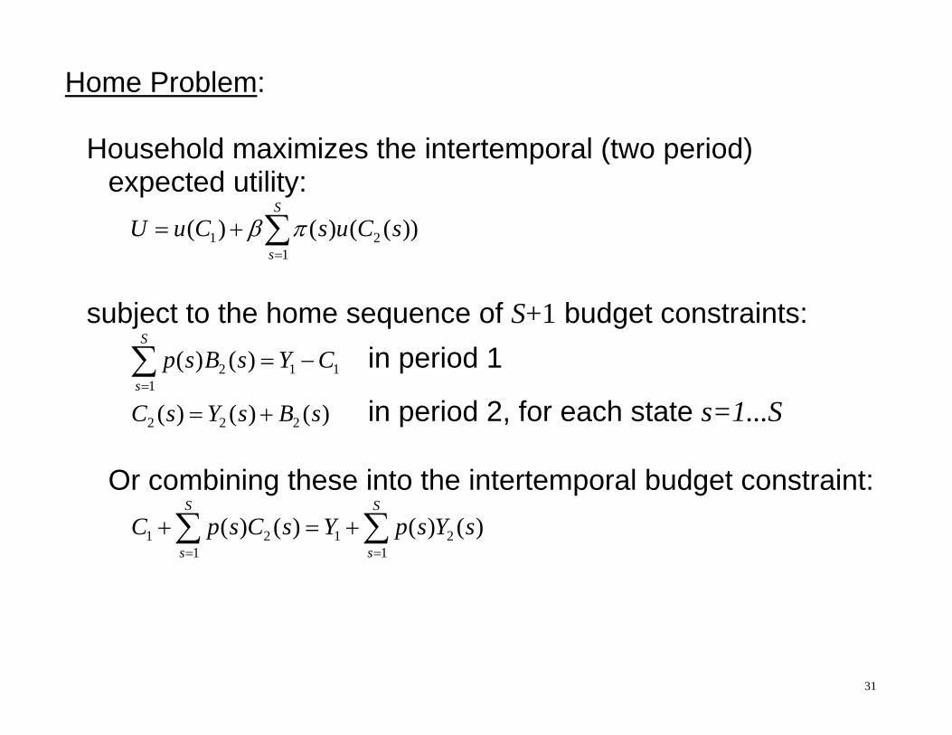
Home Problem: Household maximizes the intertemporal (two period)

expected utility: 1 2

1( ) ( ) ( ( ))

S

s

U u C s u C s

subject to the home sequence of S+1 budget constraints: 2 1 1

1( ) ( )

S

s

p s B s Y C

in period 1

2 2 2( ) ( ) ( )C s Y s B s in period 2, for each state s=1...S Or combining these into the intertemporal budget constraint: 1 2 1 2

1 1( ) ( ) ( ) ( )

S S

s s

C p s C s Y p s Y s

32

First order conditions: 1 2( ) '( ) ( ) '( ( ))p s u C s u C s for each s=1...S or rewriting this: 2

1

( ) '( ( )) ( )'( )

s u C s p su C

This is a form of intertemporal consumption smoothing. It also implies consumption smoothing across states: 2

2

( ) '( ( )) ( )( ') '( ( ')) ( ')

s u C s p ss u C s p s

An analogous problem applies to the foreign household,

and will produce analogous first order conditions. Note that the security prices in these conditions ( )p s will be

identical, since same securities being traded globally.

33

Implications: So we have the following implications:

*22

*11

( ) '( ( )) ( ) '( ( ))( )'( ) '( )

s u C s s u C sp su C u C

and

*22

*22

( ) '( ( )) ( ) ( ) '( ( ))( ') '( ( ')) ( ') ( ') '( ( '))

s u C s p s s u C ss u C s p s s u C s

This indicates that that home and foreign marginal rates of

substitution in consumption are equal – across time and states.

If we assume a standard CRRA utility function 11( )

1U C C

and define world output: *WY Y Y

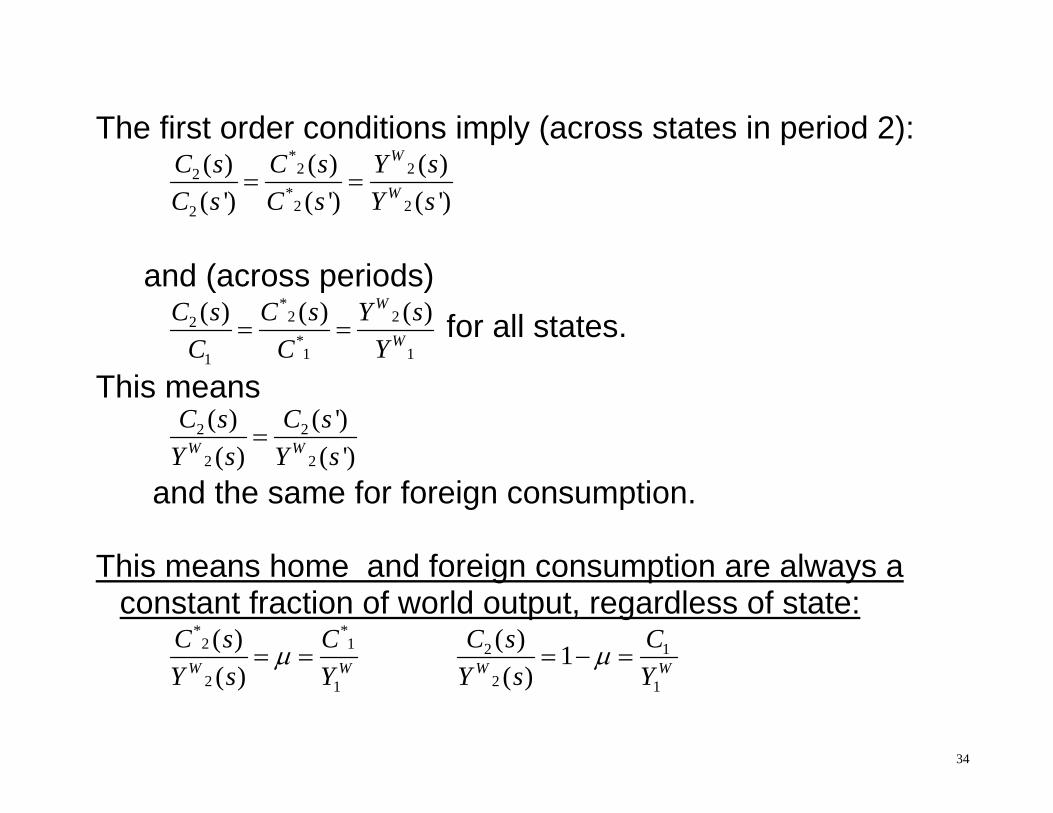
34

The first order conditions imply (across states in period 2):

*2 22

*2 22

( ) ( ) ( )( ') ( ') ( ')

W

W

C s C s Y sC s C s Y s

and (across periods)

*2 22

*1 11

( ) ( ) ( )W

W

C s C s Y sC C Y

for all states.

This means 2 2

2 2

( ) ( ')( ) ( ')W W

C s C sY s Y s

and the same for foreign consumption. This means home and foreign consumption are always a

constant fraction of world output, regardless of state:

* *2 1

2 1

( )( )W W

C s CY s Y

2 1

2 1

( ) 1( )W W

C s CY s Y

35

Or taking a ratio of the conditions above: *

1 11C C

This property of complete assets markets helps explain why

models like Backus et al (1992) have such a hard time reproducing low consumption correlations seen in the data.

36

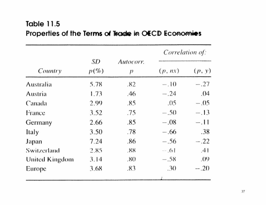
Part2: Puzzle of Relative Prices Stylized facts - Define: Terms of Trade (TOT) = price of exports / price of

imports. - The relative price data reported here is the inverse of the

usual definition of the TOT given above. - Regularities: Look at table 11.5 - The ‘terms of trade’ is highly variable: Standard deviations

are usually 2-3 times that of output. - It is also highly persistent, with an autocorrelation near 0.8.

37

38

Model - To describe relative prices, we need two types of goods. - Assume each country produces a distinctive good. Home

produces good 1; foreign good 2. Households in each country consume both goods.

- Changes in model: Use star to indicate foreign variable, H

and F to indicate good. - Two goods market clearing conditions:

ftftftftftftft

hththththththt

GGIICCYGGIICCY

*******

- Budget constraint is (using home goods as a numeraire) ...*** ftftththtfttht CCpCCYpY

39

where pt is the relative price of foreign goods in terms of home goods (pf/ph), or from home perspective, the relative price of imported goods in terms of exported goods

So pt is the inverse of the terms of trade as conventionally

defined above.

- Model home consumption as an aggregation (a function “g”) over home and foreign good:

1),( fthtfthtt CCCCgC Where start off using Cobb-Douglas for the aggregation

function. (Can use same aggregation function for investment and government demands.)

40

- Put this in utility function, and derive optimal choice between the two goods based on relative price. Intratemporal substitution again:

t

ch

cf pUU

''

- Using chain rule over the utility function, can express pt (the

inverse TOT) as the ratio of derivatives of the aggregation function over the two types of goods.

ft

ht

ht

ftht

ft

fthtt C

CC

CCgC

CCgp

1),(

/),(

- Can compute net exports (in units of home goods):

ftthtt CpCnx *

41

Results Calibrate: - Share of imports in GNP = 0.15 Simulation results for TOT: - Persistence: 0.83, similar to data. Inherit persistence from

technology shock. - Correlation of TOT with NX is negative, similar to data.

- Volatility: Sdev of TOT is much less in model than in data (data is 7X larger).

42

43

Puzzle: - So have a “relative price puzzle.” It is clear we can’t resolve this puzzle in this model just by

varying parameter values. - Discuss Ideas of how to resolve? - Recall that the intratemporal optimality condition shows that

the relative price is directly related to the ratio of imports to consumption of domestic goods.

ft

ht

ht

ftht

ft

fthtt

CC

CCCg

CCCg

p

1

),(/

),(

in percent changes fthtt CCp ~~~

44

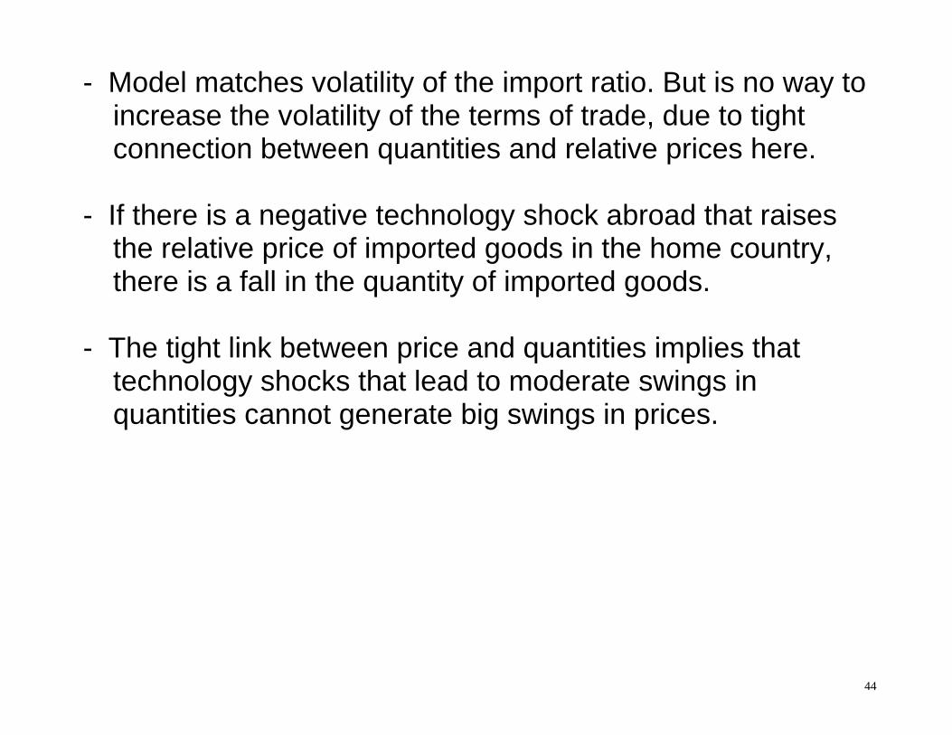
- Model matches volatility of the import ratio. But is no way to increase the volatility of the terms of trade, due to tight connection between quantities and relative prices here.

- If there is a negative technology shock abroad that raises

the relative price of imported goods in the home country, there is a fall in the quantity of imported goods.

- The tight link between price and quantities implies that

technology shocks that lead to moderate swings in quantities cannot generate big swings in prices.

45

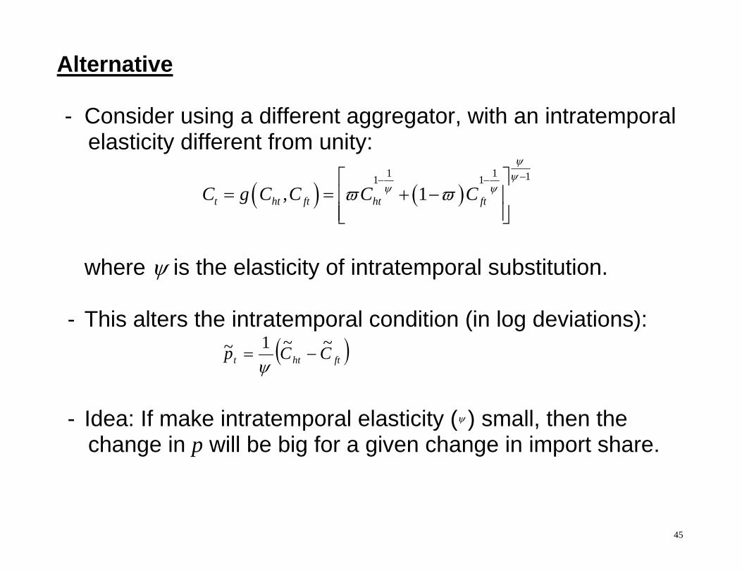
Alternative - Consider using a different aggregator, with an intratemporal

elasticity different from unity:

1 1 11 1

, 1t ht ft ht ftC g C C C C

where is the elasticity of intratemporal substitution. - This alters the intratemporal condition (in log deviations):

fthtt CCp ~~1~

- Idea: If make intratemporal elasticity ( ) small, then the

change in p will be big for a given change in import share.

46

- If goods are not very substitutable, a fall in supply of import-able good will require a very big rise in the price of import-ables to make everyone willingly consume less of them.

- But empirical estimates imply a range of 0.5 to 5 for the

elasticity; even a small value of 0.5 is not small enough to generate the observed price volatility.

Conclusion: How to break the tight link between relative prices

and quantities is a topic pursued in subsequent literature, and we will discuss this further in later lectures.

47

Backus-Smith puzzle - A related puzzle involves the comovement of international

relative prices and relative consumption levels. - The real exchange rate, q, is defined as the ratio of national

consumer price indexes in each country, foreign to home.

- Note: The national price indexes and real exchange rate are functions of the terms of traded used above (see below).

- Backus and Smith (1993) documented that correlations

between international relative consumption ratios and real exchange rates are negative or zero.

- Confirmed with more recent data, as in table below taken

from Corsetti et al (REStud 2008).

48

Aside: Derive national price index: Define the consumption index as above: 1

, ,t h t f tC C C Define the price index, P, as the minimum expenditure required

to purchase one unit of the consumption index 1

, , , ,min s.t. 1t h t t f t t h t f tP C p C C C C Implies demands:

1

1, , and

1 1h t t f t tC p C p

Plug into definition: , ,t h t t f tP C p C

1 11 1

1 1 1 1t t t t tP p p p p

49

Aside cont.: Find the real exchange rate:

Assume symmetry: foreign consumption index has weight on foreign good consumption. Note:

1* 1 1t tP p

Note: Implies consumption home bias if >½. Plug into definition of real exchange rate:

*2 1t

t tt

Pq pP

So the real exchange rate, qt, is a direct function of the (inverse) terms of trade used in the model above, pt. Note: if there is no home bias ( =1/2), so that preferences identical across countries, then q is constant at unity.

50

Annual data 1970-2001, from OECD.

51

52

- This empirical finding is contrary to economic theory, which

predicts that with full risk sharing relative consumption is perfectly positively correlated with the real exchange rate.

- Intuition: Countries with relative low prices should receive a transfer to take advantage of cheap consumption.

- This is true either for a central planner problem studied above or complete asset market. Consider again a social planner problem from above:

0

max , 1 1 , 1tt ht ht ft ft

t

E U C L U C L

where the budget constraint is written in terms of the aggregate consumption bundle, C and price index, P:

53

Budget constraint:

* * ...ht t ft t t t tY p Y PC P C First order conditions: ' *' * and 1ct t t ct t tU P U P So:

*' *

'

1 ct t

ct t

U PU P

The international ratio of marginal utilities of consumption is directly tied to the real exchange rate. In particular, assuming the marginal utility is a negative function of consumption, a rise in real exchange rate (P*/P) requires a rise in relative home consumption (C/C*).

54

Generalizations:

- This result also holds for an economy with only bonds or even financial autarky: Cole and Obstfeld (1991)

- A rise in the endowment of a country’s good usually coincides with a fall in the relative price of that good.

- This allows overall consumption in the foreign country to rise. A positive transmission.

55

- Explanations: Explaining this puzzle is ongoing in the literature. Some hypothesis in recent papers:

- Shocks to demand: such as tastes which shock the marginal utility. Or monetary policy shocks in sticky price model (Devereux and Hnatkovska, 2010)

- News shocks about future productivity have similar effect (dissertation of UCD student)

- Low elasticity of substitution between home and foreign goods with incomplete markets (Corsetti et al, RES 2008). See below.

56

Corsetti, Dedola, Leduc (RES 2008)

This paper shows that incomplete asset markets and low trade elasticities can provide an explanation for BS puzzle.

Analytical results available for case of full financial autarky and endowment. Simulations generalize the result.

Model Assumptions: - Two countries - Endowment - Each country endowed with one good; consumers

consume both national goods. - CES preferences specifying home bias and elasticity of

substitution

57

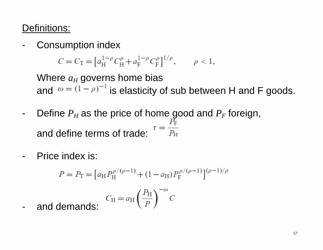
Definitions:

- Consumption index

Where aH governs home bias and is elasticity of sub between H and F goods. - Define PH as the price of home good and PF foreign,

and define terms of trade: - Price index is:

- and demands:

58

Logic of the result: - Resource constraint under autarky: PC/PH = YH .

Rewrite demand:

Take derivative with respect to terms of trade, decompose into substitution effect (SE) and income effect (IE).

- IE negative: worsening terms of trade makes home country poorer, lowering home demand for home good.

- SE positive: home good cheaper raises demand for it.

- IE can dominate if elasticity ( ) low.

59

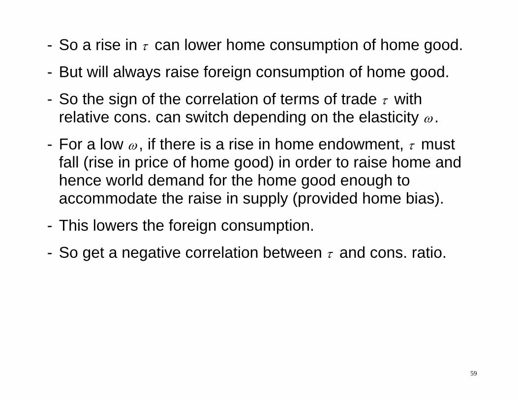
- So a rise in can lower home consumption of home good.

- But will always raise foreign consumption of home good.

- So the sign of the correlation of terms of trade with relative cons. can switch depending on the elasticity .

- For a low , if there is a rise in home endowment, must fall (rise in price of home good) in order to raise home and hence world demand for the home good enough to accommodate the raise in supply (provided home bias).

- This lowers the foreign consumption.

- So get a negative correlation between and cons. ratio.

60

More formally, manipulate balanced trade condition to get:

Use this to solve log-linearized relationship:

Conclude: Can get negative correlation if (if trade elasticity low and have home bias (aH>1/2)).

Also shows that autarky is not automatically immune to the BS puzzle: get positive correlation if elasticity too high: ie. if =1 , RER = (C=C*)

61

Simulations: Generalize model:

- Bonds in asset market - Production using labor and capital - Investment - Nontaded goods representing domestic distribution services

62

Calibration:

Macro estimates of trade elasticity vary between 0.1 and 2 (higher in trade literature)

63

Simulation Results:

64

Simulation Results:

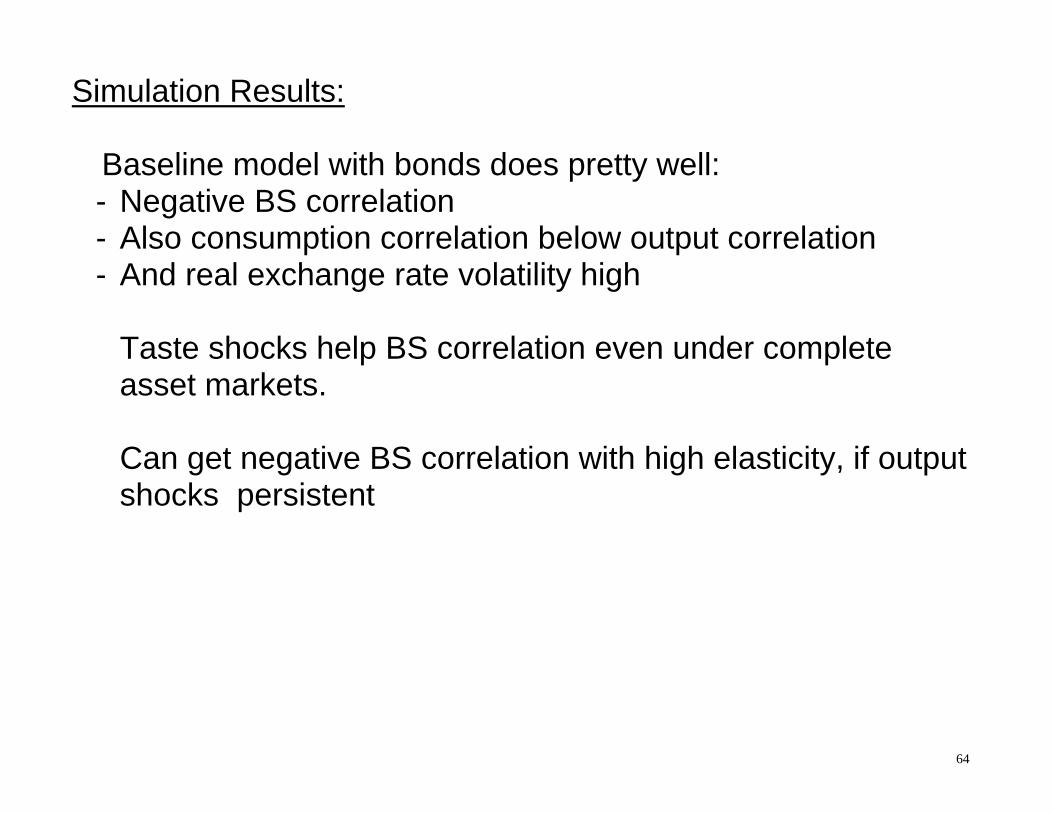
Baseline model with bonds does pretty well: - Negative BS correlation - Also consumption correlation below output correlation - And real exchange rate volatility high

Taste shocks help BS correlation even under complete asset markets.

Can get negative BS correlation with high elasticity, if output shocks persistent

65

Intuition for last finding:

- Get hump-shaped output response under endogenous labor supply and capital

- Anticipate higher future income: consumption smoothing raises current demand for home good more than supply

- This is an alternative reason why terms of trade improve upon a supply shock rather than worsen as in usual case (where BS is a puzzle).

66

Part 3: Some Examples:

A. Burstein, Kurz, Tesar (JME 2008) Question: Does international trade transmit business cycles

across countries? Past empirical work often inconclusive.

The new idea: One must distinguish different types of trade, because they have different effects on transmission.

Production sharing: as international integration increases, it is becoming for common for different stages of the production process to take place in different countries.

Observation: Countries that engage in internationalized production with each other have higher output correlations.

67

Objective: Paper models internationalized production in terms of intermediate inputs being complementary, and sees if it can replicate the positive effect on output correlation.

Observation: Production sharing has become important for US relationship with NAFTA countries, but not with EU or Japan.

Data: sales of US affiliates abroad back to US, as collected by US Bureau of Economic Analysis (BEA)

68

Observation: Trade flows associate with production sharing are more correlated with US output than are other types of trade.

69

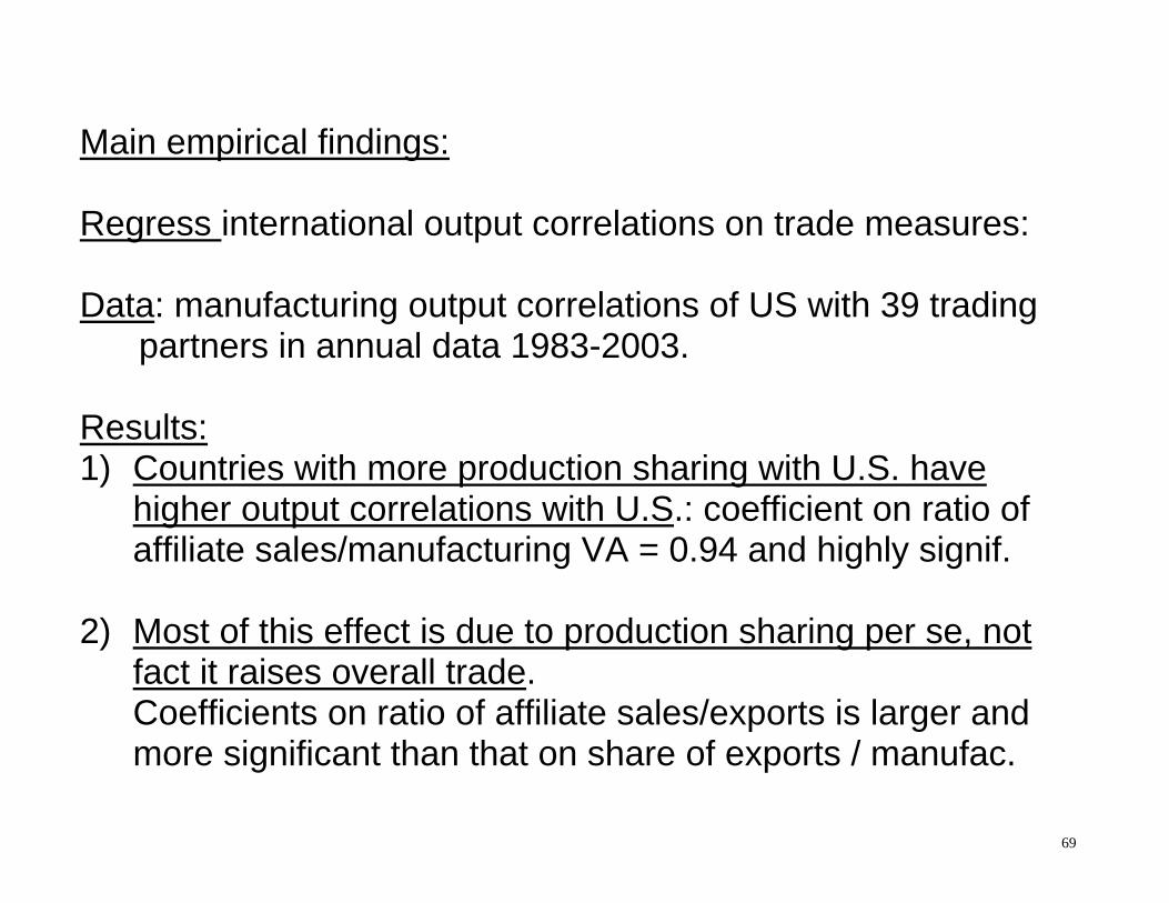
Main empirical findings: Regress international output correlations on trade measures: Data: manufacturing output correlations of US with 39 trading

partners in annual data 1983-2003. Results: 1) Countries with more production sharing with U.S. have

higher output correlations with U.S.: coefficient on ratio of affiliate sales/manufacturing VA = 0.94 and highly signif.

2) Most of this effect is due to production sharing per se, not

fact it raises overall trade. Coefficients on ratio of affiliate sales/exports is larger and

more significant than that on share of exports / manufac.

70

71

Model setup: - Extension of BKK two-country business cycle model. - Can think of the two countries as U.S. and Mexico - Introduce production sharing, in the form of complementarity

between domestic and imported intermediate inputs.

72

Multi-layered production market structure:

- Each country (i =1 or 2) uses labor and capital to produce a traded country-specific intermediate input (zi).

- These intermediate goods are combined in two ways to

create two composite final goods: 1) One final good is vertically integrated (v1), combining US and Mexican inputs as complements. Only US consumes this good. Reflects US offshoring to Mexico.

2) The other final good is horizontally integrated (xi), combining US and Mexican inputs as substitutes. Both countries consume this good.

- Distinction between goods is the elasticity of substitution.

- Model nests BKK, if the share of vertical good is set small.

73

Model equations: - Intermediate good for country i:

- Production of horizontal composite good for country i:

where the elasticity of substitution is assumed high. - Production of the vertical composite good (only country 1):

where the elasticity of substitution between inputs here is assumed smaller than .

74

- U.S. combines the two composite goods into a final tradable manufactured good using both types of composite goods:

Mexican final good is just the horizontal composite good:

- Lastly, traded good is combined with a nontraded service to

produce a final good, usable for consumption or investment:

- The resource constraint for intermediate goods: used locally to produce x1, v1, or y1

N or exported to produce x2

1 11 21 11 1

2 22 12 12 2

Nt t t t t

Nt t t t t

z x x v y

z x x v y

75

Standard preferences and resource constraints:

- Preferences like BKK:

- Resource constraint:

where

76

Definitions for comparison with data:

- Manufacturing output: T Nit it itz z y

- Volume of exports as a fraction of manufacturing output:

country 1: 1 21 1/X Ts x z

country 2: 2 12 12 2( ) /X Ts x v z - Share of country 2 exports due to production sharing

2 12 12 12/( )Ps v x v

- And country 2’s share of production share in manufac GDP

2 2P Xs x

(assumes v11 not shipped from 2 to 1, so not in export)

77

Calibration: - Mainly from BKK:

- Elasticity of sub between home and foreign intermediates in

Horizontal composite: 2. Vertical composite: 0.05

- Share of intermediate in vertical composite equal share of US imports in Mexican maquiladora gross output:

Standard stochastic simulations Conducted under alternative calibrations of trade share

( 2Xs ) and production sharing share ( 2

Ps ).

78

Simulation results: international correlation of manufac. output rises with share of trade due to production sharing

and overall trade: corr( 1 2,T Tz z ) rises with 2Ps and 2

Xs

79

Intuition: consider positive productivity shock to country 1:

- Raises supply of both horizontal and vertical composites in country 1.

- Raises demand for imports of all types from country 2

- And raises the relative price of country 2 exports.

- Some of the rise in demand for country 2 exports is offset by rise in price.

- This substitution effect due to price is smaller for vertical composite, so exports of vertical good from country 2 rise more than horizontal good.

- So there is a larger spillover to country 2 when there is a larger share of vertical goods.

80

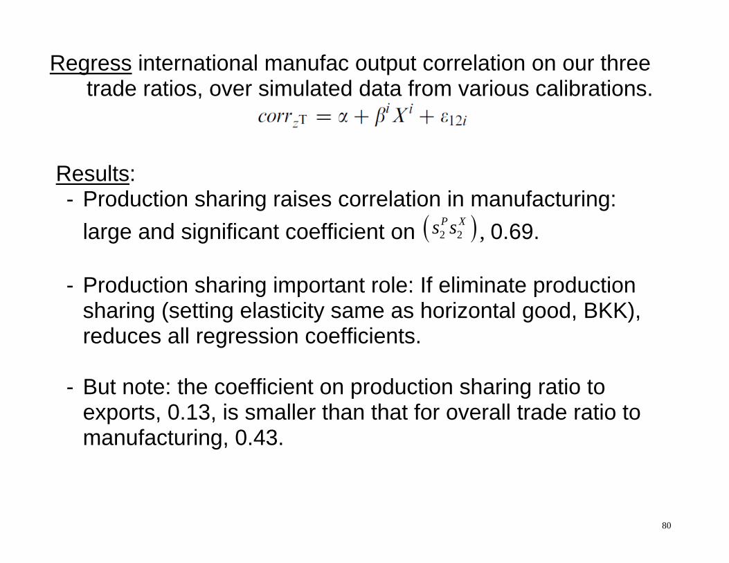
Regress international manufac output correlation on our three trade ratios, over simulated data from various calibrations.

Results:

- Production sharing raises correlation in manufacturing: large and significant coefficient on 2 2

P Xs s , 0.69.

- Production sharing important role: If eliminate production sharing (setting elasticity same as horizontal good, BKK), reduces all regression coefficients.

- But note: the coefficient on production sharing ratio to exports, 0.13, is smaller than that for overall trade ratio to manufacturing, 0.43.

81

82

Extensions and limitations:

- Is it problematic that in the model production sharing is less important than overall trade for promoting international output correlations?

- The model takes international production as exogenous, but might respond to shocks. Consider model of entry subject to fixed costs.

- Authors note that countries with shared production might be subject to more correlated productivity shocks.

83

B. Engel and Wang (2011) Some Questions: 1) What is main question addressed. What new stylized fact? 2) What would standard RBC model of BKK predict? 3) why can’t explain even if add higher real exch. rate volatility? 4) What do they add to model, and how model it? 5) What is the main result? 6) What is the intuition for the result? 7) critiques/comments? Counterfactual implications,

questionable calibrations, alternative explanations 8) Interesting implications or extensions come to mind?

104

Part 4: Effects of great recession on trade:

- Alessandria, Kaboski, and Midrigan (2010): Student presentation.

- Levchenko, Lewis and Tesar (2010):

Student presentation. Questions to consider: 1) Was the recent dramatic downturn in trade unusual?

2) Can the downturn in trade be understood in terms of standard real business cycle mechanisms?

3) Do you think we need additional frictions, such as trade financing and financial market shocks to understand the trade downturn?