lecture 2: a crash course in rSTAT 545: Introduction to computational statistics

Vinayak RaoDepartment of Statistics, Purdue University

August 25, 2016

The R programming language

From the manual,

• R is a system for statistical computation and graphics• R provides a programming language, high level graphics,interfaces to other languages and debugging facilities

It is possible to go far using R interactively

Better:

• Organize code for debugging/reproducibility/homework

1/43

The R programming language

John Chambers:

• Everything that exists is an object• Everything that happens is a function call

• typeof() gives the type or internal storage mode of an object• str() provides a summary of the R object• class() returns the object’s class

2/43

Atomic vectors

Collections of objects of the same type

Common types include: “logical”, “integer”, “double”,“complex”, “character”, “raw”

R has no scalars, just vectors of length 1

3/43

Creating vectors

One-dimensional vectors:age <- 25 # 1-dimensional vectorname <- ”Alice”; undergrad <- FALSEtypeof(age) # Note: age is a double#> [1] ”double”class(age)#> [1] ”numeric”

age <- 15L # L for long integertypeof(age)#> [1] ”integer”

4/43

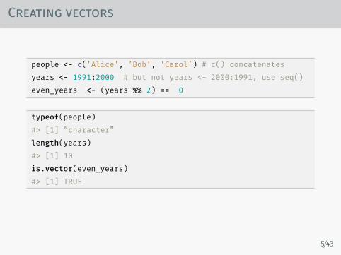
Creating vectors

people <- c(’Alice’, ’Bob’, ’Carol’) # c() concatenatesyears <- 1991:2000 # but not years <- 2000:1991, use seq()even_years <- (years %% 2) == 0

typeof(people)#> [1] ”character”length(years)#> [1] 10is.vector(even_years)#> [1] TRUE

5/43

Indexing elements of a vector

Use brackets [] to index subelements of a vectorpeople[1] # First element is indexed by 1#> [1] ”Alice”years[1:5] # Index with a subvector of integers#> [1] 1991 1992 1993 1994 1995years[c(1, 3, length(years))]#> [1] 1991 1993 2000

6/43

Indexing elements of a vector

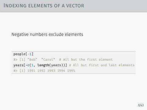
Negative numbers exclude elements

people[-1]#> [1] ”Bob” ”Carol” # All but the first elementyears[-c(1, length(years))] # All but first and last elements#> [1] 1991 1992 1993 1994 1995

6/43

Indexing elements of a vector

Index with logical vectors

even_years <- (years %% 2) == 0#> [1] FALSE TRUE FALSE TRUE FALSE TRUE FALSE TRUE FALSE TRUEyears[even_years] # Index with a logical vector#> [1] 1992 1994 1996 1998 2000

6/43

Indexing elements of a vector

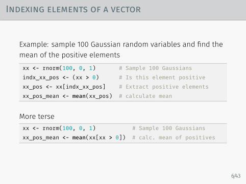
Example: sample 100 Gaussian random variables and find themean of the positive elementsxx <- rnorm(100, 0, 1) # Sample 100 Gaussiansindx_xx_pos <- (xx > 0) # Is this element positivexx_pos <- xx[indx_xx_pos] # Extract positive elementsxx_pos_mean <- mean(xx_pos) # calculate mean

More tersexx <- rnorm(100, 0, 1) # Sample 100 Gaussiansxx_pos_mean <- mean(xx[xx > 0]) # calc. mean of positives

6/43

Replacing elements of a vector

Can assign single elementspeople[1] <- ”Dave”; print(people)#> [1] ”Dave” ”Bob” ”Carol”

or multiple elementsyears[even_years] <- years[even_years] + 1#> [1] 1991 1993 1993 1995 1995 1997 1997 1999 1999 2001

(more on this when we look at recycling)years[-c(1,length(years)] <- 0#> [1] 1991 0 0 0 0 0 0 0 0 2001

7/43

Replacing elements of a vector

What if we assign to an element outside the vector?years[length(years) + 1] <- 2015years#> [1] 1991 0 0 0 0 0 0 0 0 2001 2015length(years)#> [1] 11

We have increased the vector length by 1

In general, this is an inefficient way to go about things

Much more efficient is to first allocate the entire vector

8/43

Recycling

vals <- 1:6#> [1] 1 2 3 4 5 6vals + 1#> [1] 2 3 4 5 6 7

vals + c(1, 2)#> [1] 2 4 4 6 6 8

Can repeat explicitly toorep(c(1, 2),3)#> [1] 1 2 1 2 1 2rep(c(1, 2),each=3)#> [1] 1 1 1 2 2 2

9/43

Some useful R functions

seq(), min(), max(), length(), range(), any(), all(),

Comparison operators: <, <=, >, >=, ==, !=

Logical operators: &&, ||, !, &, |, xor()

is.logical(), is.integer(), is.double(), is.character()as.logical(), as.integer(), as.double(), as.character()

‘Coercion’ often happens implicitly in function calls:sum(rnorm(10) > 0)

10/43

Lists (generic vectors) in R

Elements of a list can be any R object (including other lists)

Lists are created using list():> car <- list(”Ford”, ”Mustang”, 1999, TRUE)> length(car)

Can have nested lists:# car, house, cat and sofa are other lists> possessions <- list(car, house, cat, sofa, ”3000USD”)

11/43

Indexing elements of a list

Use brackets [] and double brackets [[]]

Brackets [] return a sublist of indexed elements

12/43

Indexing elements of a list

Use brackets [] and double brackets [[]]

Brackets [] return a sublist of indexed elements

> car[1][[1]][1] ”Ford”

> typeof(car[1])[1] ”list”

12/43

Indexing elements of a list

Use brackets [] and double brackets [[]]

Double brackets [[]] return element of list

> car[[1]][1] ”Ford”

> typeof(car[[1]])[1] ”character”

12/43

Named lists

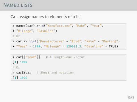
Can assign names to elements of a list

> names(car) <- c(”Manufacturer”, ”Make”, ”Year”,+ ”Mileage”, ”Gasoline”)# Or> car <- list(”Manufacturer” = ”Ford”, ”Make” = ”Mustang”,+ ”Year” = 1999, ”Mileage” = 120021.3, ”Gasoline” = TRUE)

13/43

Named lists

Can assign names to elements of a list

> names(car) <- c(”Manufacturer”, ”Make”, ”Year”,+ ”Mileage”, ”Gasoline”)# Or> car <- list(”Manufacturer” = ”Ford”, ”Make” = ”Mustang”,+ ”Year” = 1999, ”Mileage” = 120021.3, ”Gasoline” = TRUE)

> car[[”Year”]] # A length-one vector[1] 1999# Or> car$Year # Shorthand notation[1] 1999

13/43

Object attributes

names() is an instance of an object attribute

These store useful information about the object

Other common attributes: class, dim and dimnames.

Many have specific accessor functions e.g. class() or dim()

You can create your own

14/43

Matrices and arrays

Are two- and higher-dimensional collections of objects

These have an appropriate dim attribute> my_mat <- 1:6 # vector[1] 1 2 3 4 5 6> dim(my_mat) <- c(3,2) # 3 rows and 2 columns> my_mat

[,1] [,2][1,] 1 4[2,] 2 5[3,] 3 6

> my_arr <- array(1:8, c(2,2,2)), , 1

[,1] [,2][1,] 1 3[2,] 2 4

, , 2[,1] [,2]

[1,] 5 7[2,] 6 8

15/43

Matrices and arrays

Are two- and higher-dimensional collections of objects

These have an appropriate dim attribute> my_mat <- 1:6 # vector[1] 1 2 3 4 5 6> dim(my_mat) <- c(3,2) # 3 rows and 2 columns> my_mat

[,1] [,2][1,] 1 4[2,] 2 5[3,] 3 6

Equivalently (and better)> my_mat <- matrix(1:6, nrow = 3, ncol = 2) # ncol is redundant

> my_arr <- array(1:8, c(2,2,2)), , 1

[,1] [,2][1,] 1 3[2,] 2 4

, , 2[,1] [,2]

[1,] 5 7[2,] 6 8

15/43

Matrices and arrays

Are two- and higher-dimensional collections of objects

These have an appropriate dim attribute> my_arr <- array(1:8, c(2,2,2)), , 1

[,1] [,2][1,] 1 3[2,] 2 4

, , 2[,1] [,2]

[1,] 5 7[2,] 6 8

15/43

Matrices and arrays

Useful functions include

• typeof(), class(), str()

• dim(), nrow(), ncol()

• is.matrix(), as.matrix(), …

16/43

Matrices and arrays

A vector/list is NOT an 1-d matrix (no dim attribute)> is.matrix(1:6)[1] FALSE

Use drop() to eliminate empty dimensions> my_mat <- array(1:6, c(2,3,1)) # dim(my_mat) is (2,3,1), , 1

[,1] [,2] [,3][1,] 1 3 5[2,] 2 4 6

> my_mat <- array(1:6, c(2,3,1)) # dim(my_mat) is (2,3,1), , 1

[,1] [,2] [,3][1,] 1 3 5[2,] 2 4 6> my_mat <- drop(my_mat) # dim is now (2,3)

[,1] [,2] [,3][1,] 1 3 5[2,] 2 4 6

17/43

Matrices and arrays

A vector/list is NOT an 1-d matrix (no dim attribute)> is.matrix(1:6)[1] FALSE

Use drop() to eliminate empty dimensions> my_mat <- array(1:6, c(2,3,1)) # dim(my_mat) is (2,3,1), , 1

[,1] [,2] [,3][1,] 1 3 5[2,] 2 4 6> my_mat <- drop(my_mat) # dim is now (2,3)

[,1] [,2] [,3][1,] 1 3 5[2,] 2 4 6

17/43

Indexing matrices and arrays

> my_mat[2,1] # Again, use square brackets[1] 2

Excluding an index returns the entire dimension> my_mat[2,][1] 2 4 6> my_arr[1,,1] # slice along dim 2, with dims 1, 3 equal to 1[1] 6 8

Usual ideas from indexing vectors still apply> my_mat[c(2,3),]

[,1] [,2][1,] 2 5[2,] 3 6

18/43

Column-major order

We saw how to create a matrix from an array> my_mat <- matrix(1:6, nrow = 3, ncol = 2)

[,1] [,2][1,] 1 4[2,] 2 5[3,] 3 6

In R matrices are stored in column-major order(like Fortran, and unlike C and Python)> my_mat[1:6][1] 1 2 3 4 5 6

19/43

Recycling

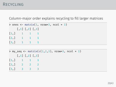
Column-major order explains recycling to fill larger matrices> ones <- matrix(1, nrow=3, ncol = 3)

[,1] [,2] [,3][1,] 1 1 1[2,] 1 1 1[3,] 1 1 1

> my_seq <- matrix(c(1,2,3), nrow=3, ncol = 3)[,1] [,2] [,3]

[1,] 1 1 1[2,] 2 2 2[3,] 3 3 3

20/43

Data frames

Very common and convenient data structures

Used to store tables:

Columns are variables and rows are observations

Age PhD GPAAlice 25 TRUE 3.6Bob 24 TRUE 3.4Carol 21 FALSE 3.8

An R data frame is a list of equal length vectors and specialconvenience syntax

21/43

Data frames

> df <- data.frame(age = c(25L,24L,21L),PhD = c(T,T,F),GPA = c(3.6,2.4,2.8))

> dfage PhD GPA

1 25 TRUE 3.62 24 TRUE 2.43 21 FALSE 2.8> typeof(df)[1] ”list”> class(df)[1] ”data.frame”

> str(df) # Try yourself

22/43

Data frames

Since data frames are lists, we can use list indexing

Can also use matrix indexing (more convenient)> df[2,3][1] 2.4> df[2,]

age PhD GPA2 24 TRUE 2.4> df$GPA[1] 3.6 2.4 2.8

• list functions apply as usual• matrix functions are also interpreted intuitively

23/43

Data frames

Many datasets are data frames and many packages expectdataframes> library(”datasets”)> class(mtcars)[1] ”data.frame”

> head(mtcars) # Print part of a large objectmpg cyl disp hp drat wt qsec vs am gear

Mazda RX4 21.0 6 160 110 3.90 2.620 16.46 0 1 4Mazda RX4 Wag 21.0 6 160 110 3.90 2.875 17.02 0 1 4Datsun 710 22.8 4 108 93 3.85 2.320 18.61 1 1 4Hornet 4 Drive 21.4 6 258 110 3.08 3.215 19.44 1 0 3Hornet Sportabout 18.7 8 360 175 3.15 3.440 17.02 0 0 3Valiant 18.1 6 225 105 2.76 3.460 20.22 1 0 3

24/43

if statements

Allow conditional execution of statementsif( condition1 ) {

statement1} else if( condition2 ) {

statement2} else {

statement3}

25/43

Logical operators

!: logical negation

& and &&: logical ‘and’

| and ||: logical ‘or’

& and | perform elementwise comparisons on vectors

&& and ||:

• evaluate from left to right• look at first element of each vector• evaluation proceeds only until the result is determined

26/43

explicit looping: for(), while() and repeat()

for(elem in vect) { # Can be atomic vector or listDo_stuff_with_elem # over successive elements of vect

}

x <- 0for(ii in 1:50000) x <- x + log(ii) # Horriblex <- sum(log(1:50000)) # Much more simple and efficient!> system.time({x<-0; for(i in 1:50000) x[i] <- i})

user system elapsed0.048 0.000 0.048

> system.time(x <- log(sum(1:50000))user system elapsed0.001 0 0.002

27/43

Vectorization

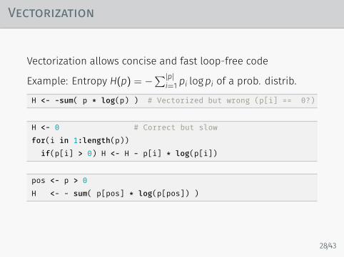
Vectorization allows concise and fast loop-free code

Example: Entropy H(p) = −∑|p|

i=1 pi logpi of a prob. distrib.

H <- -sum( p * log(p) ) # Vectorized but wrong (p[i] == 0?)

H <- 0 # Correct but slowfor(i in 1:length(p))

if(p[i] > 0) H <- H - p[i] * log(p[i])

pos <- p > 0H <- - sum( p[pos] * log(p[pos]) )

28/43

While loops

while( condition ) {stuff # Repeat stuff while condition evaluates to TRUE

}

If stuff doesn’t affect condition, we loop forever.

Then, we need a break statement. Useful if many conditionswhile( TRUE ) { # Or use ‘repeat { ... }’

stuff1if( condition1 ) breakstuff2if( condition2 ) break

}

29/43

The *apply family

Useful functions for repeated operations on vectors, lists etc.

Sample usage:# Calc. mean of each element of my_listrslt_list <- lapply(my_list, FUN = mean)

Stackexchange has a nice summary: [url]

Note (Circle 4 of the R inferno):

• These are not vectorized operations but are loop-hiding• Cleaner code, but comparable speeds to explicit for loops

30/43

R functions

R comes with its own suite of built-in functions

• An important part of learning R is learning the vocabularySee e.g. http://adv-r.had.co.nz/Vocabulary.html

Non-trivial applications require you build your own functions

• Reuse the same set of commands• Apply the same commands to different inputs• Cleaner, more modular code• Easier testing/debugging

31/43

Creating functions

Create functions using function:my_func <- function( formal_arguments ) body

The above statement creates a function called my_func

formal_arguments comma separated namesdescribes inputs my_func expects

function_body a statement or a blockdescribes what my_func does with inputs

32/43

An example function

normalize_mtrx <- function( ip_mat, row = TRUE ) {# Normalizes columns to add up to one if row = FALSE# If row = TRUE or row not specified, normalizes columns

if(!is.mat(ip_mat)) {warning(”Expecting a matrix as input”);return(NULL)

}# You can define objects inside a function# You can even define other functionsrslt <- if(row) ip_mat / rowSums(ip_mat) else

t( t(ip_mat) / colSums(ip_mat))}

n_mtrx <- normalize_mtrx(mtrx)

33/43

Argument matching

Proceeds by a three-pass process

• Exact matching on tags• Partial matching on tags: multiple matches gives an error• Positional matching

Any remaining unmatched arguments triggers an error

34/43

Environments in R

R follows what is called lexical scoping

Lexical scoping:

• To evaluate a symbol R checks current environment• If not present, move to parent environment and repeat• Value of the variable at the time of calling is used• Assignments are made in current environment

Here, environments are those at time of definition

Where the function is defined (rather than how it is called)determines which variables to use

Values of these variables at the time of calling are used

35/43

Scoping in R

> x <- 5; y <- 6> func1 <- function(x) {x + 1}> func1(1)

> func2 <- function() {x + 1}> func2()> x <- 10; func2() # use new x or x at the time of definition?

> func3 <- function(x) {func1(x)}> func3(2)

> func4 <- function(x) {func2()}> func4(2) # func2 uses x from calling or global environment?

36/43

Scoping in R

For more on scoping, see (Advanced R, Hadley Wickham)

The bottomline

• Avoid using global variables• Always define and use clear interfaces to functions• Warning: you are always implicitly using global objects in R

> ’+’ <- function(x,y) x*y # Open a new RStudio session!> 2 + 10

37/43

Creating functions

R’s base graphics supports some plotting commands

E.g. plot(), hist(), barplot()

Extending these standard graphics to custom plots is tedious

ggplot is much more flexible, and pretty

•• View different graphs as sharing common structure• Grammar of graphics breaks everything down into a set ofcomponents and rules relating them,

Install like you’d install any other package:install.packages(’ggplot2’)library(ggplot2)

38/43

Plotting in base R

> str(diamonds)’data.frame’: 53940 obs. of 10 variables:$ carat : num 0.23 0.21 0.23 0.29 0.31 0.24 0.24 0.26 ...$ cut : Ord.factor w/ 5 levels ”Fair”<”Good”<..: 5 4 2 ...$ color : Ord.factor w/ 7 levels ”D”<”E”<”F”<”G”<..: 2 2 ...$ clarity: Ord.factor w/ 8 levels ”I1”<”SI2”<”SI1”<..: 2 3 ...$ depth : num 61.5 59.8 56.9 62.4 63.3 62.8 62.3 61.9 ...$ table : num 55 61 65 58 58 57 57 55 61 61 ...$ price : int 326 326 327 334 335 336 336 337 337 338 ...$ x : num 3.95 3.89 4.05 4.2 4.34 3.94 3.95 4.07 ...$ y : num 3.98 3.84 4.07 4.23 4.35 3.96 3.98 4.11 ...$ z : num 2.43 2.31 2.31 2.63 2.75 2.48 2.47 2.53 ...

plot(diamonds$carat, diamonds$price) # plot(x,y)

39/43

Plotting in ggplot

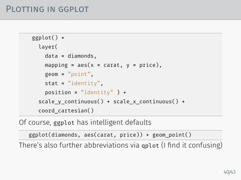
ggplot() +layer(

data = diamonds,mapping = aes(x = carat, y = price),geom = ”point”,stat = ”identity”,position = ”identity” ) +

scale_y_continuous() + scale_x_continuous() +coord_cartesian()

Of course, ggplot has intelligent defaultsggplot(diamonds, aes(carat, price)) + geom_point()

There’s also further abbreviations via qplot (I find it confusing)

40/43

Layers

ggplot produces an object that is rendered into a plot

This object consists of a number of layers

Each layer can get own inputs or share arguments to ggplot()

Add another layer to previous plot:ggplot(diamonds, aes(x=carat, y = price)) + geom_point()

+ geom_line(stat= ”smooth”, color=”blue”, size=5, alpha=0.7)

41/43

More Examples

ggplot(diamonds, aes(x=carat, y = price,colour=cut)) +geom_point() +geom_line(stat= ”smooth”, size=5, alpha= 0.7)

ggplot(diamonds, aes(x=carat, y = price,colour=cut)) +geom_point() +geom_line(stat= ”smooth”, method=lm, size=5, alpha= 0.7) +scale_x_log10()+ scale_y_log10()

ggplot(diamonds, aes(x=carat, fill=cut)) +geom_histogram(alpha=0.7, binwidth=.4, color=”black”,position=”dodge”) + xlim(0,2) + coord_cartesian(xlim=c(.1,5))

42/43

A more complicated example

Kowno

Wilna

SmorgoniMoiodexno

Gloubokoe

Minsk

Studienska

Polotzk

Bobr

Witebsk

Orscha

Mohilow

SmolenskDorogobouge

Wixma

Chjat Mojaisk

Moscou

Tarantino

Malo−Jarosewii

54.0

54.5

55.0

55.5

24 28 32 36

direction

A

R

survivors

1e+05

2e+05

3e+05

‘A Layered Grammar of Graphics’, Hadlay Wickham, Journal ofComputational and Graphical Statistics, 2010

ggplot documentation: http://docs.ggplot2.org/current/

Search ‘ggplot’ on Google Images for inspiration

Play around to make your own figures

43/43