
Lecture 18 FFT
61
Dr. Iman Abuel Maaly 1 م ي ح ر ل ا ن م ح ر ل له ا ل م ا س بDigital Signal processing Lecture (18) Fast Fourier Transform Algorithms (FFT) University of Khartoum Department of Electrical and Electronic Engineering Fourth Year
-
Upload
mohamed-alser -
Category
Documents
-
view
234 -
download
2
description
fast fouir transfomatim
Transcript of Lecture 18 FFT

Dr. Iman Abuel Maaly 1
الرحيم الرحمن الله بسم
Digital Signal processingLecture (18)
Fast Fourier Transform Algorithms (FFT)
2009-2010
University of Khartoum
Department of Electrical and Electronic Engineering
Fourth Year
Introduction
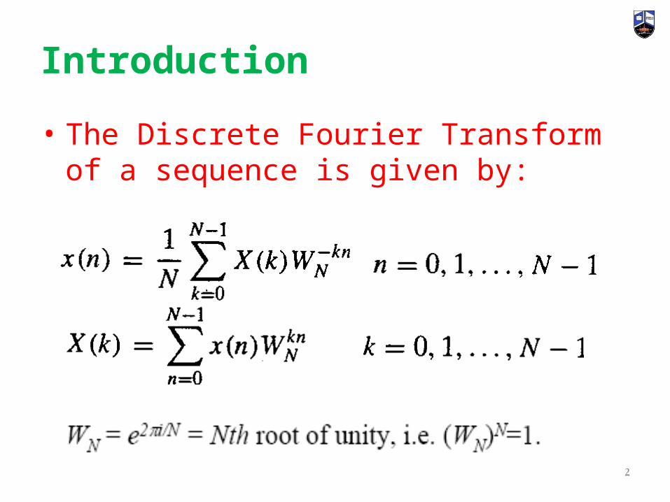
• The Discrete Fourier Transform of a sequence is given by:
2

How much computations does it require?
For a complex valued sequence x(n) of N points, DFT may be expressed as :
3
Introduction
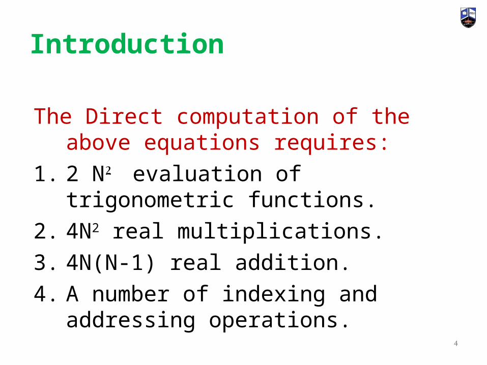
The Direct computation of the above equations requires:
1. 2 N2 evaluation of trigonometric functions.
2. 4N2 real multiplications.
3. 4N(N-1) real addition.
4. A number of indexing and addressing operations.
4
Introduction

Can we speed this up?.......
• Exploit the symmetry and periodicity property of the phase factor
• Symmetry property:
• Periodicity property:
• This led to Divide and conquer approach.
5

Efficient computation of t he DFT: Fast Fourier Transform FFT• There are two approaches for the efficient
computation of the DFT1.The Divide and Conquer Approach.2.An approach based on the formulation of the
DFT as a linear filtering operation on the data:a) Goertzel Algorithmb) Chirp-z transform algorithm
6

• This approach is based on the decomposition of an N-point DFT into successively smaller DFTs.
• Let N= L M• x(n) can be stored in a one dimensional array
indexed by n, 0≤ n≤ N-1, or as a two-dimensional array indexed by l, m where
• 0≤ l≤ L-1 and 0≤ m≤ M-1
7
Divide and conquer approach to Computation of the DFT.

Divide and conquer approach.• A one dimensional array
• A two dimensional array
8

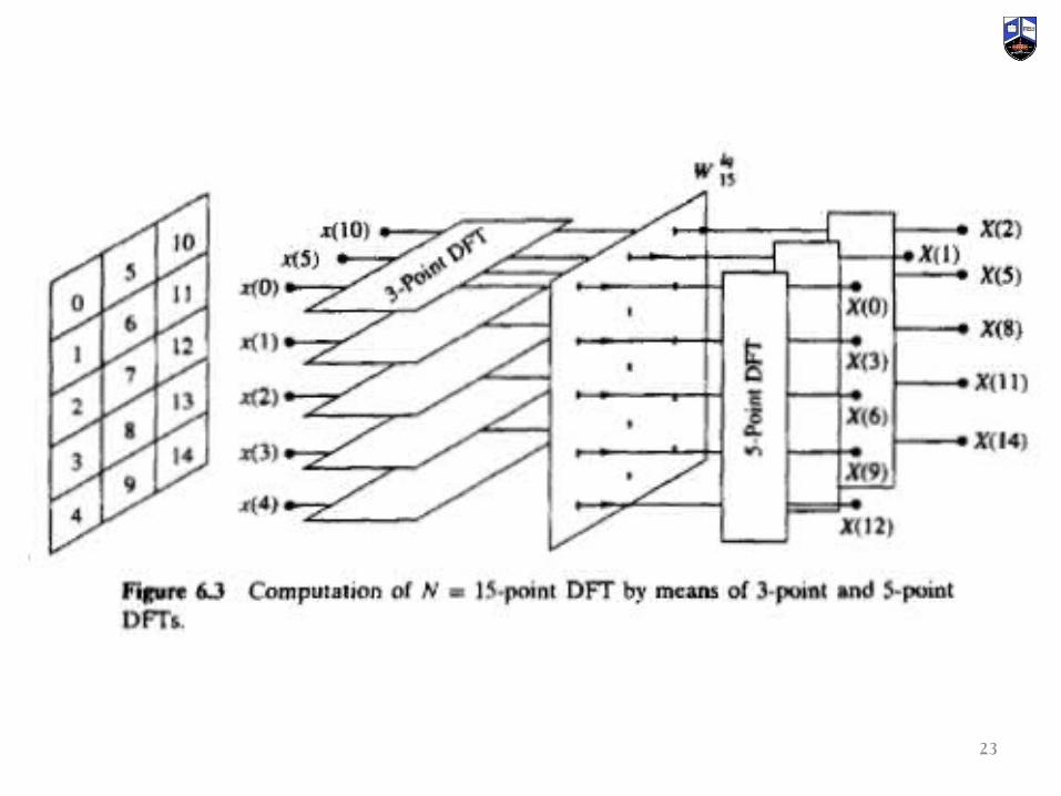
• Suppose that we select the mapping
• n= Ml+m
• See the figure below in which the first row contains the first M elements and the second row contains the next M elements an so on.
9
Divide and conquer approach to Computation of the DFT.

10
n = Ml +m
Divide and conquer approach to Computation of the DFT.
Row wise base
11
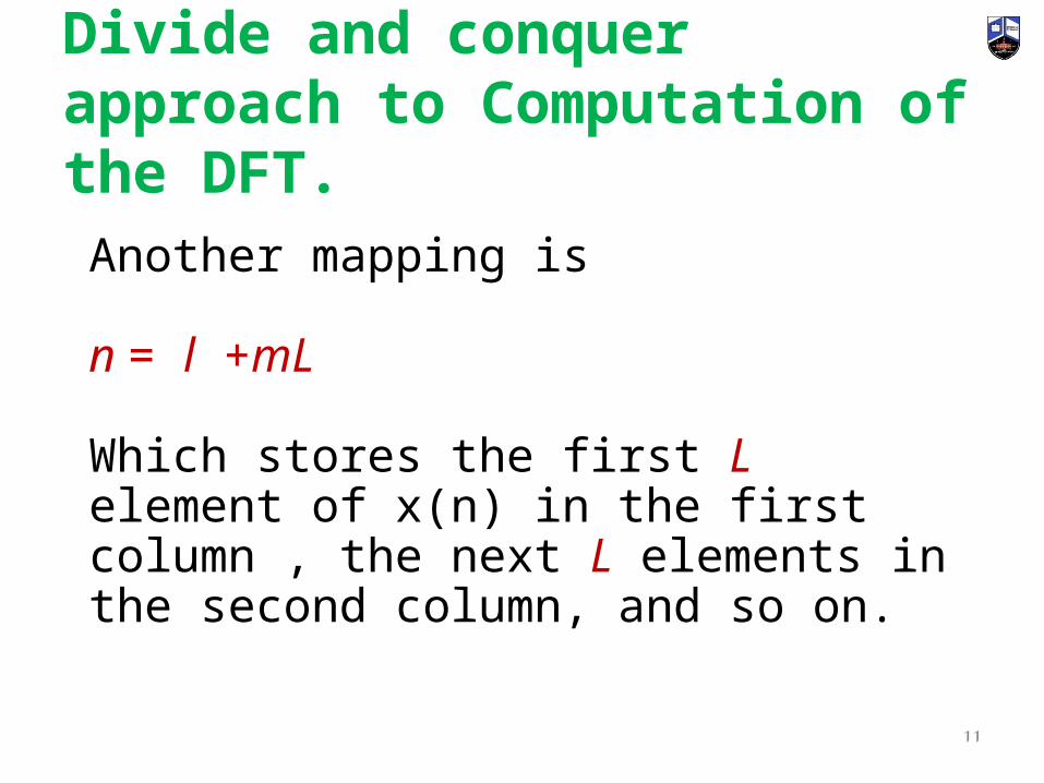
Another mapping is
n = l +mL
Which stores the first L element of x(n) in the first column , the next L elements in the second column, and so on.
Divide and conquer approach to Computation of the DFT.

Divide and conquer approach.
12
n = l +mLColumn wise base

• The same arrangement can be used to store the computed DFT values.
• Select the mapping of the index k into p and q where:
0≤ p≤ L-1 , 0≤ q≤ M-1• We can select either • k = Mp +q ( a row-wise basis)or • k = qL +p (a column-wise basis)
13
Divide and conquer approach.

• If x(n) is mapped into x(l,m)
and X(k) is mapped into X(p,q),
then we adopt a column wise basis for x(n) and a row-wise basis for X(k)
• i.e.,
n = l +mL
k = Mp +q
14
Divide and conquer approach.

15
• Then the DFT can be expressed as a double sum over the elements of the rectangular array multiplied by the corresponding phase factors.
1
0
1
0
))((),(),(M
m
L
l
lmLqMpNWmlxqpX
But
lqN
MplN
mLqN
MLmpN
lmLqMpN WWWWW ))((

16
1MLmpNW
mqM
mqLN
mqLN WWW /
plL
plMN
MplN WWW /
However
lqN
MplN
mLqN
MLmpN
lmLqMpN WWWWW ))((
lqN
plL
mqM
lmLqMpN WWWW ))((
17
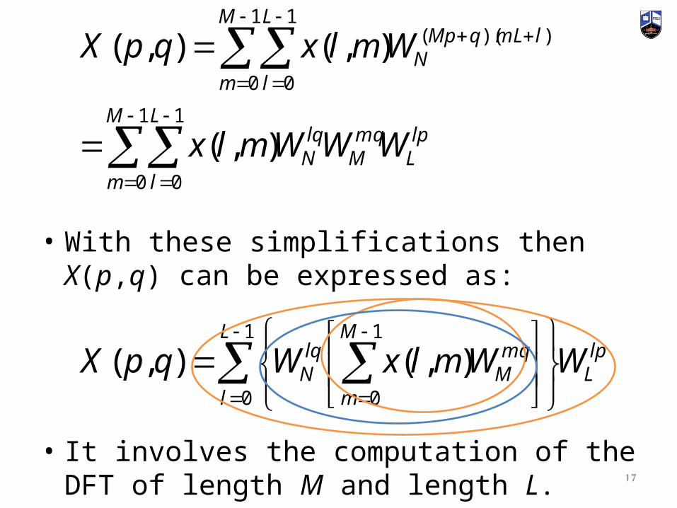
• With these simplifications then X(p,q) can be expressed as:
• It involves the computation of the DFT of length M and length L.
lpL
L
l
M
m
mqM
lqN WWmlxWqpX
1
0
1
0
),(),(
lpL
mqM
M
m
L
l
lqN
M
m
L
l
lmLqMpN
WWWmlx
WmlxqpX
1
0
1
0
1
0
1
0
))((
),(
),(),(

1. First we compute the M-point DFTs
For each of the rows l =0,1,2,…..L-1
2. Second, we compute a new rectangular array G(l,q) defined as
3. Finally, we compute the L-point DFTs
for each column q = 0, 1,…,M-1 of the array G(l,q)18
10,),(),(1
0
MqWmlxqlFM
m
mqM
10
10,),(),(
Mqand
LlqlFWqlG lqN
lpL
L
l
WqlGqpX
1
0
),(),(
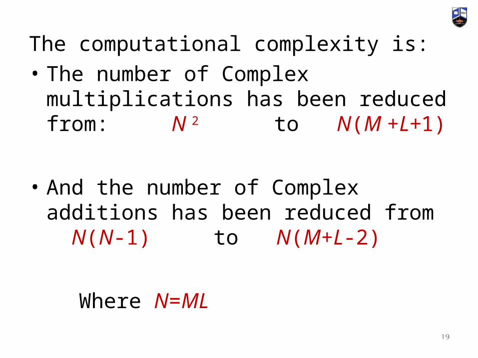
The computational complexity is:
• The number of Complex multiplications has been reduced from: N 2 to N(M +L+1)
• And the number of Complex additions has been reduced from N(N-1) to N(M+L-2)
Where N=ML
19
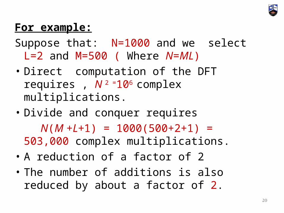
For example:
Suppose that: N=1000 and we select L=2 and M=500 ( Where N=ML)
• Direct computation of the DFT requires , N 2
=106 complex multiplications.
• Divide and conquer requires
N(M +L+1) = 1000(500+2+1) = 503,000 complex multiplications.
• A reduction of a factor of 2
• The number of additions is also reduced by about a factor of 2.
20
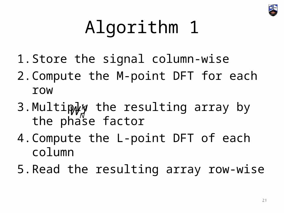
Algorithm 1
1. Store the signal column-wise
2. Compute the M-point DFT for each row
3. Multiply the resulting array by the phase factor
4. Compute the L-point DFT of each column
5. Read the resulting array row-wise
21
lqNW

Algorithm 2
1. Store the signal row-wise
2. Compute the L-point DFT for each column
3. Multiply the resulting array by the phase factor
4. Compute the M-point DFT of each row
5. Read the resulting array column-wise
22
pmNW
23
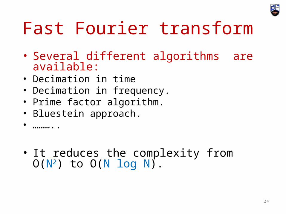
Fast Fourier transform • Several different algorithms are available:• Decimation in time• Decimation in frequency.• Prime factor algorithm.• Bluestein approach.• ………..
• It reduces the complexity from O(N2) to O(N log N).
24

Radix-2 FFT Algorithm
• If N is highly composite, N= r1 r2 r3 …… rv
where ri are prime .
• If r1 =r2 =r3≡ rv so that N = r v ,the DFT of size r is called the radix of the FFT section.
In Radix-2 algorithm In Radix-2 algorithm r r =2.=2.
25

Radix-2 FFT Algorithm (cont)
• Let us consider the computation of the N = 2v point DFT by the divide-and conquer approach. We select L=2 and M=N/2.
• We split the N-point data sequence x(n) into two N/2-point data sequences f1(n) and f2(n), corresponding to the even-numbered and odd-numbered samples of x(n), respectively, that is,
26
{x(0), x(2), x(4), …}
{x(1), x(3), x(5), …}
Radix-2 FFT Algorithm (cont)
• Thus f1(n) and f2(n) are obtained by decimating x(n) by a factor of 2, and hence the resulting FFT algorithm is called a decimation-in-time algorithm.
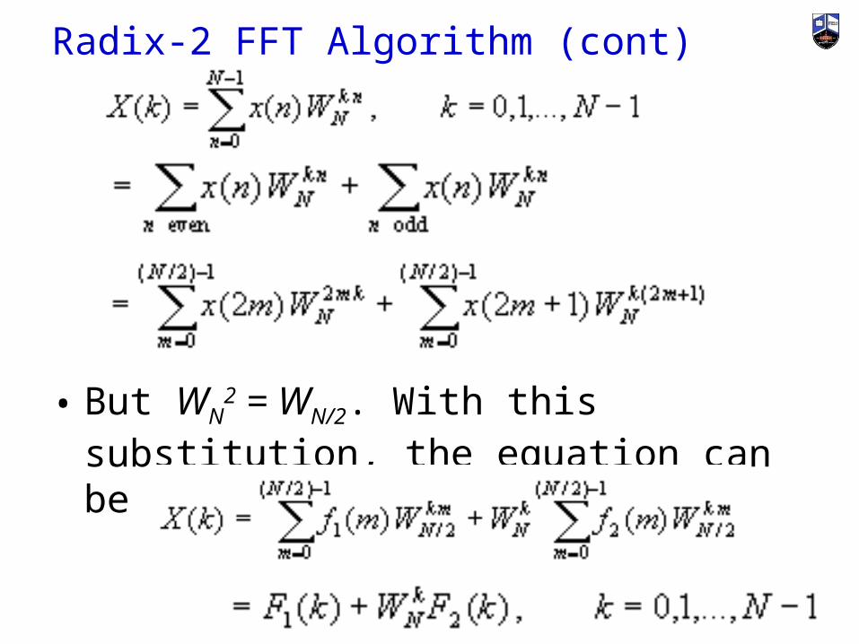
• Now the N-point DFT can be expressed in terms of the DFTs of the decimated sequences as follows:
27
Radix-2 FFT Algorithm (cont)
• But WN2 = WN/2. With this substitution, the
equation can be expressed as
28

Radix-2 FFT Algorithm (cont)
• where F1(k) and F2(k) are the N/2-point DFTs of the sequences f1(m) and f2(m), respectively.
• Since F1(k) and F2(k) are periodic, with period N/2, we have
• F1(k+N/2) = F1(k) and F2(k+N/2) = F2(k).
• In addition, the factor WNk+N/2 = -WN
k. Hence the equation may be expressed as
29

Radix-2 FFT Algorithm (cont)Computation:
• We observe that the direct computation of F1(k) requires (N/2)2 complex multiplications. The same applies to the computation of F2(k).
• Furthermore, there are N/2 additional complex multiplications required to compute WN
kF2(k).
• Hence the computation of X(k) requires 2(N/2)2 + N/2 = N 2/2 + N/2 complex multiplications. 30
Radix-2 FFT Algorithm (cont)
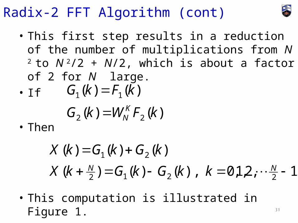
• This first step results in a reduction of the number of multiplications from N 2 to N 2/2 + N/2, which is about a factor of 2 for N large.
• If
• Then
• This computation is illustrated in Figure 1.31
)()(
)()(
22
11
kFWkG
kFkGK
N
1,2,1,0),()()(
)()()(
2212
21
NN kkGkGkX
kGkGkX

Radix-2 FFT Algorithm (cont)
32
Figure 1. First step in the decimation-in-time algorithm

Radix-2 FFT Algorithm (cont)
• We can repeat the sequence for each f1(n) and f2(n).
• Thus f1(n) would result in the two N/4 point sequences,
• And f2(n) yields:
33
1,2,1,0),12()(
1,2,1,0),2()(
4112
4111
N
N
nnfnv
nnfnv
1,2,1,0),12()(
1,2,1,0),2()(
4222
4221
N
N
nnfnv
nnfnv
Radix-2 FFT Algorithm (cont)
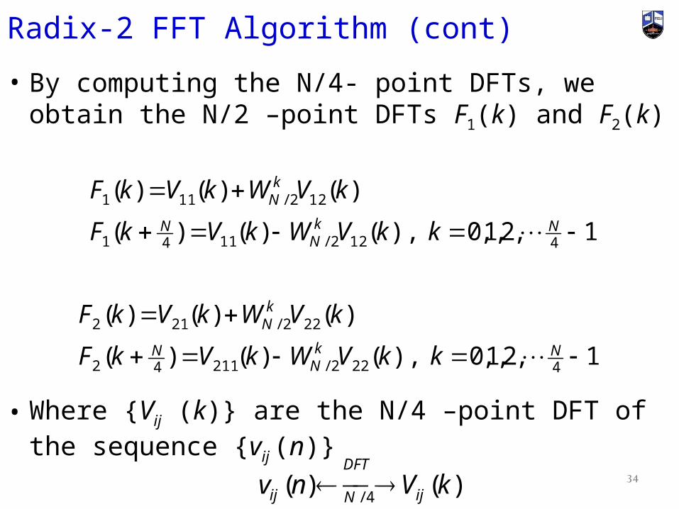
• By computing the N/4- point DFTs, we obtain the N/2 –point DFTs F1(k) and F2(k)
• Where {Vij (k)} are the N/4 –point DFT of the sequence {vij (n)} 34
1,2,1,0),()()(
)()()(
4122/1141
122/111
Nk
NN
kN
kkVWkVkF
kVWkVkF
1,2,1,0),()()(
)()()(
4222/21142
222/212
Nk
NN
kN
kkVWkVkF
kVWkVkF
)()(4/
kVnv ij
DFT
Nij

Radix-2 FFT Algorithm (cont)Computation:
• {Vij (k)} requires 4(N/4)2 complex multiplications and hence
• The computation of F1(k) and F2(k) can be accomplished with complex multiplications
• To compute X(k) from F1(k) and F2(k) requires N/2 complex multiplications
• The total is computation is reduced by a factor of 2
35
24
2 NN
NNNNN
4224
22

Radix-2 FFT Algorithm (cont)Computation:
• The decimation of the data sequence can be repeated again and again until the resulting sequences are reduced to one-point sequences. For N = 2v,
• this decimation can be performed v = log2N times.
• Thus the total number of complex multiplications is reduced to (N/2)log2N.
• The number of complex additions is N log2N.36

Radix-2 FFT Algorithm (cont)
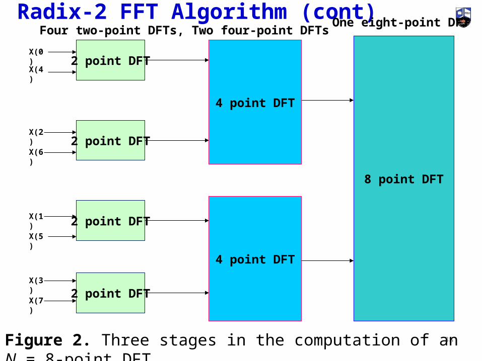
• For illustrative purposes, Figure 2 depicts the computation of N = 8 point DFT.
• We observe that the computation is performed in three stages,
• beginning with the computations of four two-point DFTs,
• then two four-point DFTs,
• and finally, one eight-point DFT.
37
2 point DFTX(0)
X(4)
X(2)
X(6)
X(1)
X(5)
X(3)
X(7)
4 point DFT
8 point DFT
4 point DFT
2 point DFT
2 point DFT
2 point DFT
38
Radix-2 FFT Algorithm (cont)
Figure 2. Three stages in the computation of an N = 8-point DFT.
Four two-point DFTs, Two four-point DFTsOne eight-point DFT
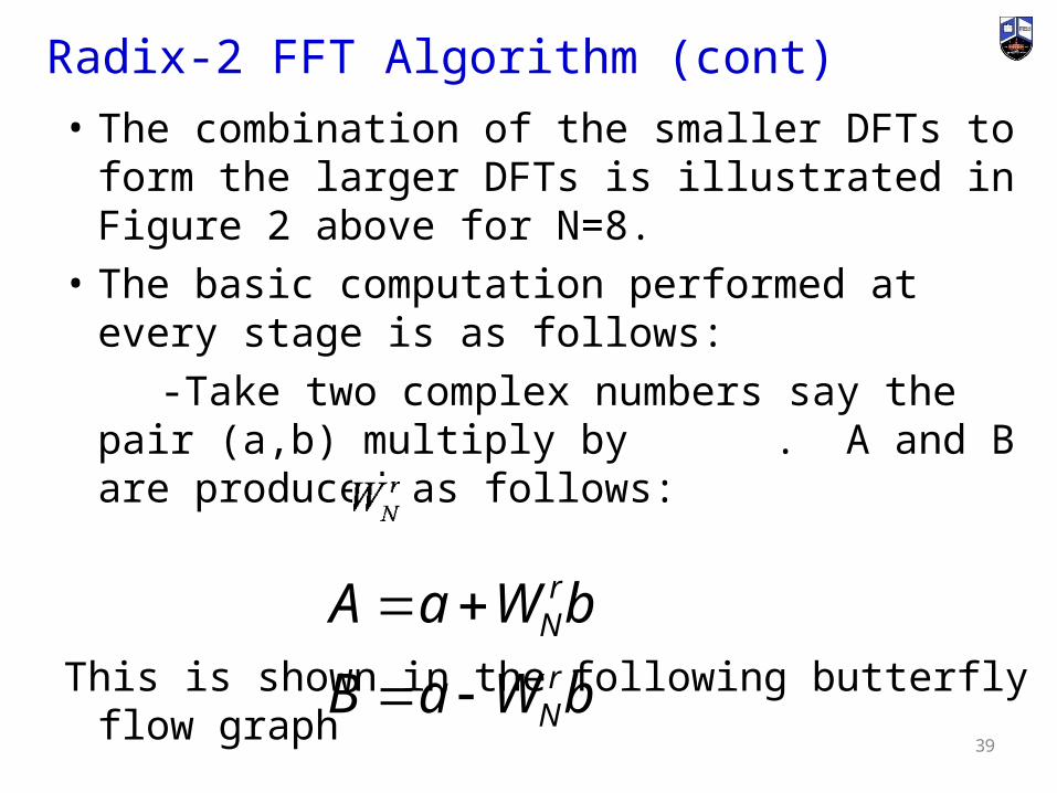
Radix-2 FFT Algorithm (cont)• The combination of the smaller DFTs to form the
larger DFTs is illustrated in Figure 2 above for N=8.
• The basic computation performed at every stage is as follows:
-Take two complex numbers say the pair (a,b) multiply by . A and B are produced as follows:
This is shown in the following butterfly flow graph
39
bWaB
bWaAr
N
rN

Radix-2 FFT Algorithm (cont)
• Figure .3 Basic butterfly computation in the decimation-in-time FFT algorithm.
40

Radix-2 FFT Algorithm (cont)
41Figure .4 Eight-point decimation-in-time FFT algorithm.

Radix-2 FFT Algorithm (cont)
• Storage
• For each stage we store (A,B) after computation in the same location as (a,b)
• The required storage is of size 2N to store N complex number of the computation of each stage.
• The computations are done in place.
42

Radix-2 FFT Algorithm (cont)• Order of Input Data
• An important observation is concerned with the order of the input data sequence after it is decimated (v-1) times.
• For example, if we consider the case where N = 8, we know that the first decimation yeilds the sequence
• x(0), x(2), x(4), x(6), x(1), x(3), x(5), x(7),
• and the second decimation results in the sequence
• x(0), x(4), x(2), x(6), x(1), x(5), x(3), x(7).
43

Radix-2 FFT Algorithm (cont)
• Order of Input Data
• This shuffling of the input data sequence has a well-defined order as can be ascertained from observing Figure .5, which illustrates the decimation of the eight-point sequence.
•
44

45
Order of Input DataShuffling of data and bit reversal
Figure .5 a Shuffling of the data and bit reversal
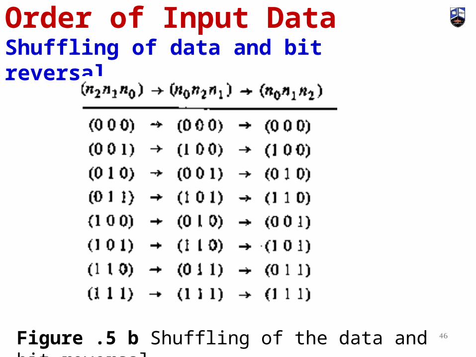
Order of Input DataShuffling of data and bit reversal
46Figure .5 b Shuffling of the data and bit reversal
Radix-2 FFT Algorithm (cont)
• Thus we say that that data x(n) after decimation is stored in bit reversal order.
• After the input data stored in bit reversal order and the butterfly computation performed in place the resultant DFT sequence X(k) is easily obtained in natural order. (k=0,1,2,,…, N-1)
We can arrange the FFT algorithm such that-input data is left in natural order
- DFT will occur in reversal order
47

Radix-2 Algorithm Decimation in Frequency
48

Radix-2 Algorithm Decimation in Frequency
• Another important radix-2 FFT algorithm, called the decimation-in-frequency algorithm, is obtained by using the divide-and-conquer approach. (N=LM , M=2 and L=N/2)
• To derive the algorithm, we begin by splitting the DFT formula into two summations, one of which involves the sum over the first N/2 data points and the second sum involves the last N/2 data points.
49

Radix-2 FFT Algorithm (Decimation in Frequency(cont)• Thus we obtain:
50

Radix-2 FFT Algorithm (Decimation in Frequency(cont)
• Now, let us split (decimate) X(k) into the even- and odd-numbered samples. Thus we obtain
• where we have used the fact that WN2 = WN/2
51

Radix-2 FFT Algorithm (Decimation in Frequency(cont)
• The computational procedure above can be repeated through decimation of the N/2-point DFTs X(2k) and X(2k+1).
• The entire process involves v = log2N stages of decimation, where each stage involves N/2 butterflies of the type shown in Figure 6.
52
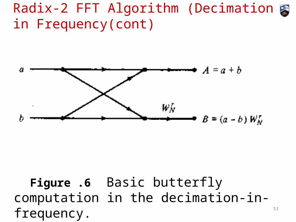
Radix-2 FFT Algorithm (Decimation in Frequency(cont)
Figure .6 Basic butterfly computation in the decimation-in-frequency.
53

Radix-2 FFT Algorithm (Decimation in Frequency (cont)Computations
• Consequently, the computation of the N-point DFT via the decimation-in-frequency FFT requires (N/2)log2N complex multiplications and N log2N complex additions, just as in the decimation-in-time algorithm.
• For illustrative purposes, the eight-point decimation-in-frequency algorithm is given in Figure 7.
•
54
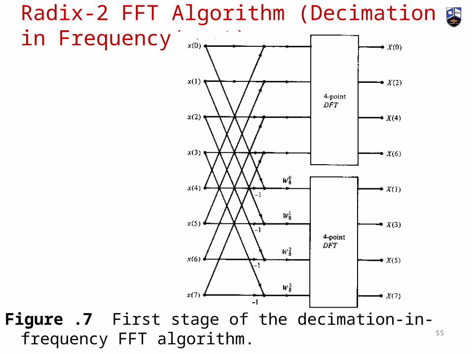
Radix-2 FFT Algorithm (Decimation in Frequency(cont)
Figure .7 First stage of the decimation-in-frequency FFT algorithm.
55

Radix-2 FFT Algorithm (Decimation in Frequency(cont)
56Figure .8 N = 8-piont decimation-in-frequency FFT algorithm.
Radix-2 FFT Algorithm (Decimation in Frequency(cont)
• We observe from Figure .8 that the input data x(n) occurs in natural order, but the output DFT occurs in bit-reversed order.
• We also note that the computations are performed in place.
• However, it is possible to reconfigure the decimation-in-frequency algorithm so that the input sequence occurs in bit-reversed order while the output DFT occurs in normal order.
57

Radix-2 FFT Algorithm (Decimation in Frequency(cont)
• Furthermore, if we abandon the requirement that the computations be done in place, it is also possible to have both the input data and the output DFT in normal order.
58
Applications
59
The Fast Fourier Transform (FFT) is one of the most important tools in Digital Signal Processing.
First, the FFT can calculate a signal's frequency spectrum. This is a direct examination of information encoded in the frequency, phase, and amplitude of the component sinusoids.

• Second, the FFT can find a system's frequency response from the system's impulse response, and vice versa. This allows systems to be analyzed in the frequency domain, just as convolution allows systems to be analyzed in the time domain.
• Third, the FFT can be used as an intermediate step in more elaborate signal processing techniques. The classic example of this is FFT convolution, an algorithm for convolving signals that is hundreds of times faster than conventional methods.
60

الله ،،، وفقكم
61
تعالى الله بحمد تم