• Lecture 16

• Readings on Simple & Multiple Regression

• Outliers

• Interaction Effects

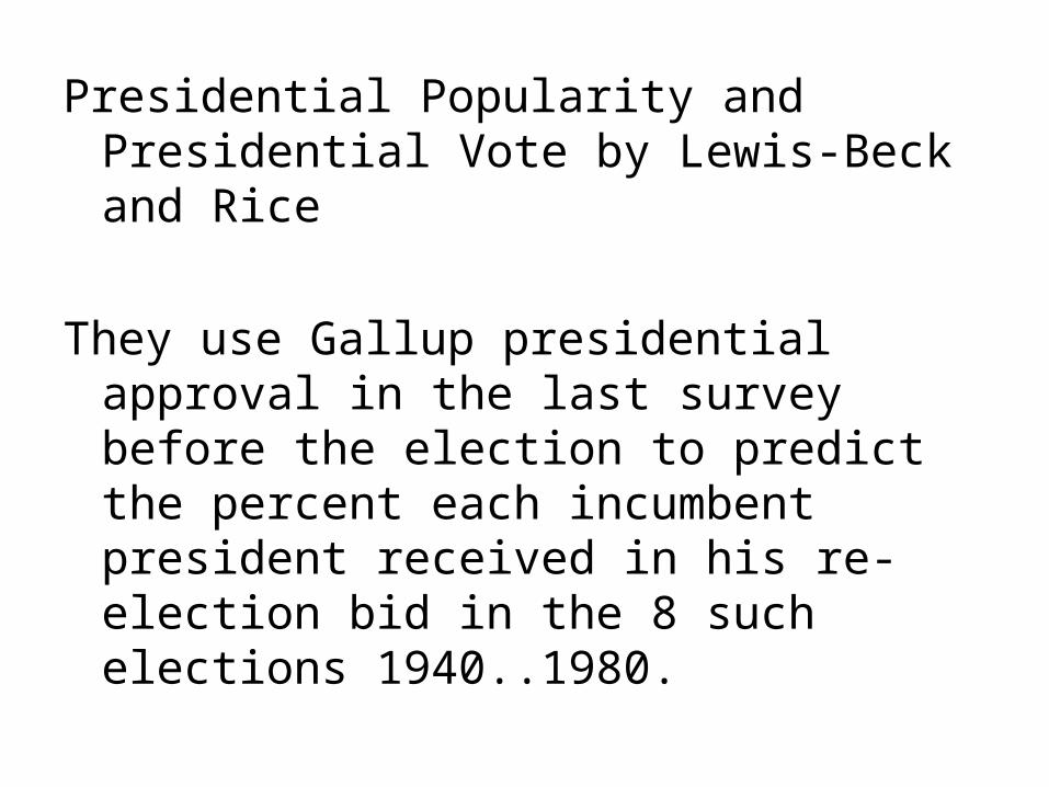
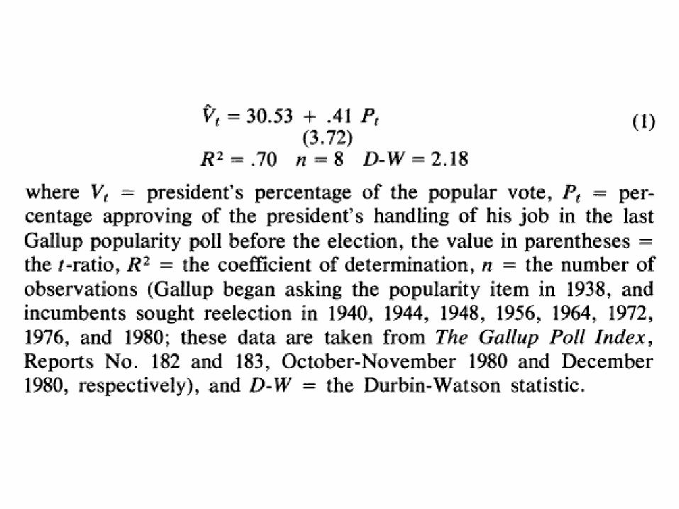
Presidential Popularity and Presidential Vote

by Lewis-Beck and Rice

They use Gallup presidential approval in the last survey before the election to predict the percent each incumbent president received in his re-election bid in the 8 such elections 1940..1980.

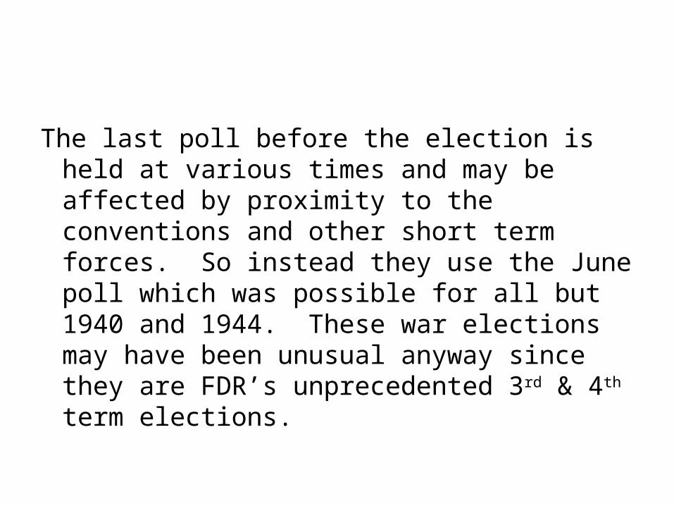
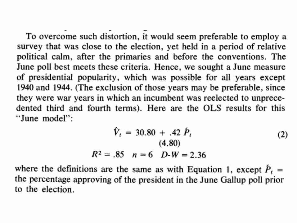
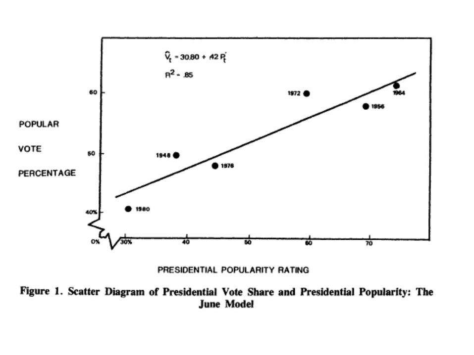
The last poll before the election is held at various times and may be affected by proximity to the conventions and other short term forces. So instead they use the June poll which was possible for all but 1940 and 1944. These war elections may have been unusual anyway since they are FDR’s unprecedented 3rd & 4th term elections.

The paper we just looked at was a very early publication in this area. Predicting national presidential vote outcomes has become a cottage industry with a reasonable number of scholars submitting their model and prediction of the result before each election.

This is intrinsically an interesting topic and since there are very few data points the models must be kept quite simple with few independent variables.

Here I’ll just give an example of one model for 2004 by Alan Abramowitz

V=50.3 + .81*GDP+.113*NETAPP-4.7*TFC

V=predicted major party vote for incumbent party

GDP=growth rate of real gross domestic product during the first two quarters of the year

NETAPP=incumbent president’s approval-disapproval in the final Gallup Poll in June

TFC=0 of pres party has controlled the White House for one term and 1 if two terms or more

The national economy also has an impact on congressional elections.

Now let’s look at:

Economic Conditions and the Forgotten Side of Congress: A Foray into US Senate Elections

Hibbing & Alford

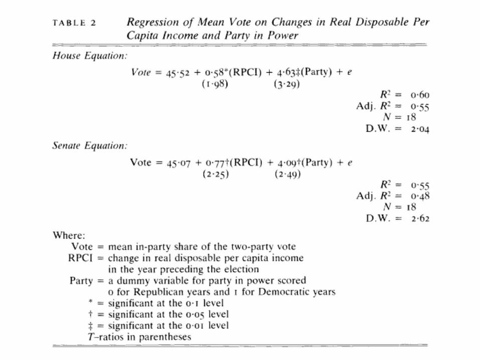
They wish to compare the impact of economic conditions on the electoral support for congressional candidates of the president’s party.

Here they look separately at House and Senate elections 1946—1980.

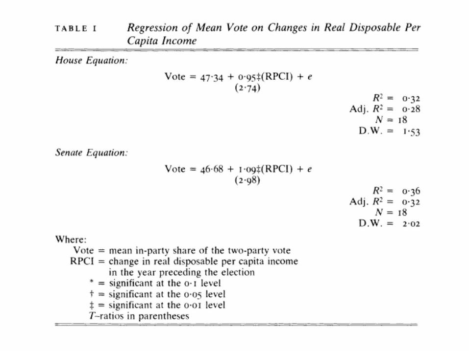
If one party is stronger than the other during the period, we may misestimate the effect of the economy on vote. When a control for party is included the coefficient on the economy is smaller than in the simple bivariate regression. The coefficients are still sig although now only at the .1 and .05 levels. The R square increases.

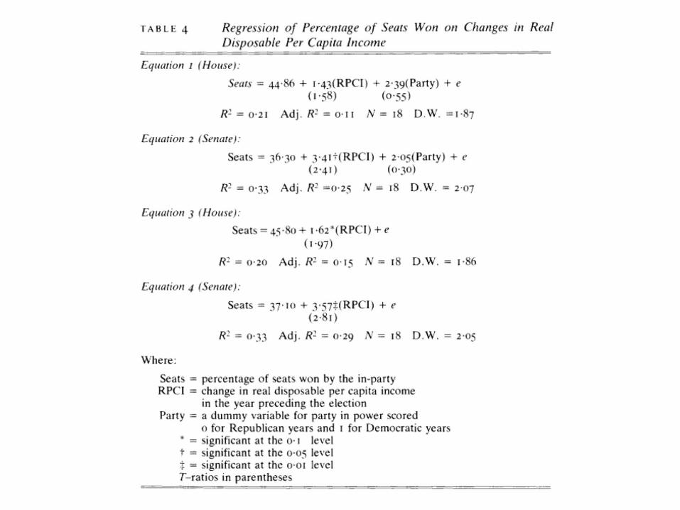
Now the authors change the dependent variable to look at the percent of seats won by the president’s party.

Here we see that the coefficient for the economy in the Senate equation is much larger than in the House equation.

For the Senate a 1% change in RPCI yields a 3.5% change in the proportion of seats. Or with about 33 Senate elections in a year—one seat difference.

For the House a 1% change yields less than half that % change.

• For an updated model, we can examine one by Gary Jacobson.

• For the House, he predicts the percentage of seats gained or lost by the president’s party.

• %seat change=

• -17.70-.76 Exposure+1.29 change in real income per capita+.25 pres approval

• Adjusted Rsq=.70 N of elections=29

• Next we can take a look at the final regression article by Gary Jacobson.

• The Effect of the AFL-CIO’s “Voter Education” Campaigns on the 1996 House Elections

Jacobson indicates that the Republican takeover of the House in 1994 provoked a swift response from labor.

• Outliers.• We didn’t have time to cover the section

that dealt with outliers and non-linear regression

• There is one article in that section that I did want to mention. Earlier in the course we read several articles on electoral competitiveness. One of these was by Jacobson.

• To refresh your memory, Jacobson argued that marginals had not vanished. Although incumbents were winning by larger margins, vote margins were more variable and just about as many incumbents were losing office as had previously.

• Bauer and Hibbing update Jacobson’s data adding the 1980s. They argue that incumbents are safer. The 1970s are an outlier—an unusual decade.

• The 1970s included Watergate, several House scandals, and a major redistricting.—altogether an atypical decade.

• Jacobson’s conclusions rested on few instances of actual incumbent defeats. A longer time period provided a better perspective.

Dummy Variables and Interactive Terms

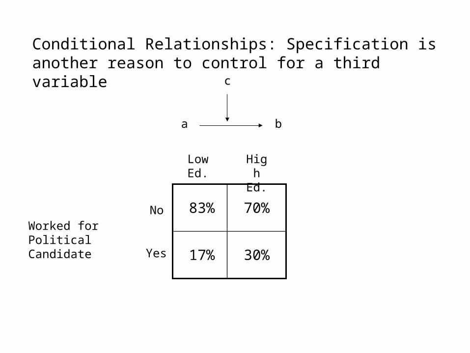
70%83%

17% 30%

Conditional Relationships: Specification is another reason to control for a third variable

a b

c

Low Ed.

High Ed.

No

Yes

Worked for Political Candidate

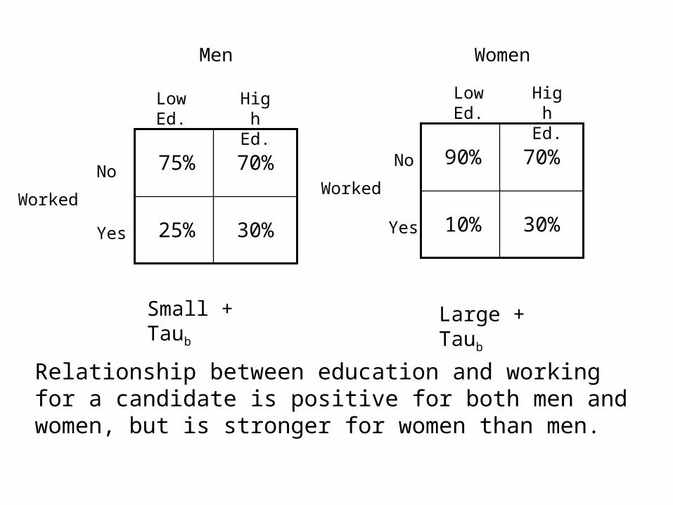
70%75%

25% 30%

70%90%

10% 30%

Low Ed.

Low Ed.

High Ed.

High Ed.

NoNo

Yes Yes

WorkedWorked

Small + Taub Large + Taub

Men Women

Relationship between education and working for a candidate is positive for both men and women, but is stronger for women than men.

• We haven’t talked about how to look at conditional relationships with regression.

• We know from our earlier work, that better educated constituencies are more likely to be represented by women in the legislature.

• We could ask whether this relationship is stronger in the South than in the rest of the US.

• Women are more likely to be elected outside the south. Education might make more difference in the south.

• We could simply do one regression for the south and another for the rest of the country.

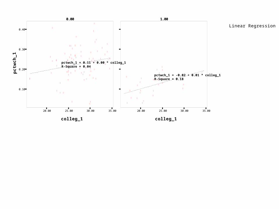
Linear Regression

20.00 25.00 30.00 35.00

colleg_1

0.10

0.20

0.30

0.40

pct

wch

_1

pctwch_1 = 0.11 + 0.00 * colleg_1R-Square = 0.04

0.00 1.00

20.00 25.00 30.00 35.00

colleg_1

pctwch_1 = -0.02 + 0.01 * colleg_1R-Square = 0.18

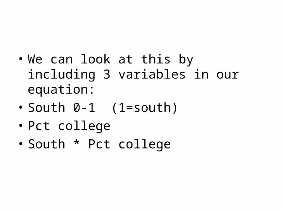
• We can look at this by including 3 variables in our equation:

• South 0-1 (1=south)

• Pct college

• South * Pct college

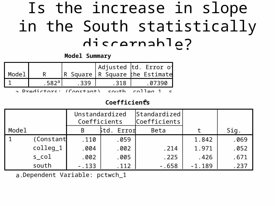
Is the increase in slope in the South statistically discernable?

• Model Summary

.582a .339 .318 .07390Model1

R R SquareAdjustedR Square

Std. Error ofthe Estimate

Predictors: (Constant), south, colleg_1, s_cola.

Coefficientsa

.110 .059 1.842 .069

.004 .002 .214 1.971 .052

.002 .005 .225 .426 .671

-.133 .112 -.658 -1.189 .237

(Constant)

colleg_1

s_col

south

Model1

B Std. Error

UnstandardizedCoefficients

Beta

StandardizedCoefficients

t Sig.

Dependent Variable: pctwch_1a.

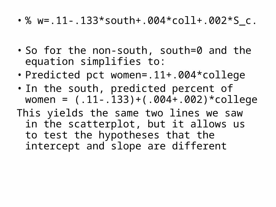
• % w=.11-.133*south+.004*coll+.002*S_c.

• So for the non-south, south=0 and the equation simplifies to:

• Predicted pct women=.11+.004*college• In the south, predicted percent of women

= (.11-.133)+(.004+.002)*collegeThis yields the same two lines we saw in the

scatterplot, but it allows us to test the hypotheses that the intercept and slope are different