211

LECTURE 14: DEVELOPING THE EQUATIONS OFMOTION FOR TWO-MASS VIBRATION EXAMPLES

Figure 3.47 a. Two-mass, linear vibration system with springconnections. b. Free-body diagrams. c. Alternative free-bodydiagram.

212

(3.123)

(3.122)

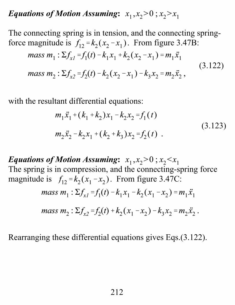
Equations of Motion Assuming:

The connecting spring is in tension, and the connecting spring-force magnitude is . From figure 3.47B:

with the resultant differential equations:

Equations of Motion Assuming: The spring is in compression, and the connecting-spring forcemagnitude is . From figure 3.47C:

Rearranging these differential equations gives Eqs.(3.122).

213

(3.124)

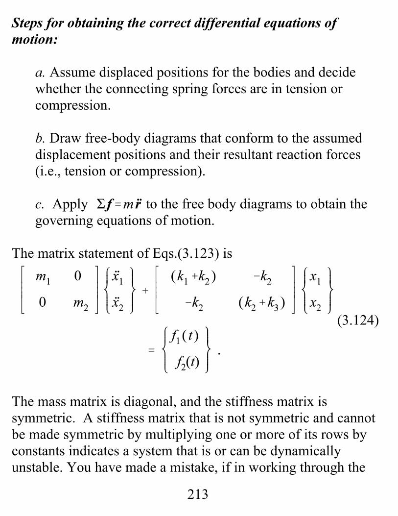
Steps for obtaining the correct differential equations ofmotion:

a. Assume displaced positions for the bodies and decidewhether the connecting spring forces are in tension orcompression.

b. Draw free-body diagrams that conform to the assumeddisplacement positions and their resultant reaction forces(i.e., tension or compression).

c. Apply to the free body diagrams to obtain thegoverning equations of motion.

The matrix statement of Eqs.(3.123) is

The mass matrix is diagonal, and the stiffness matrix issymmetric. A stiffness matrix that is not symmetric and cannotbe made symmetric by multiplying one or more of its rows byconstants indicates a system that is or can be dynamicallyunstable. You have made a mistake, if in working through the

214

example problems, you arrive at a nonsymmetric stiffnessmatrix. Also, for a neutrally-stable system, the diagonal entriesfor the mass and stiffness matrices must be greater than zero.

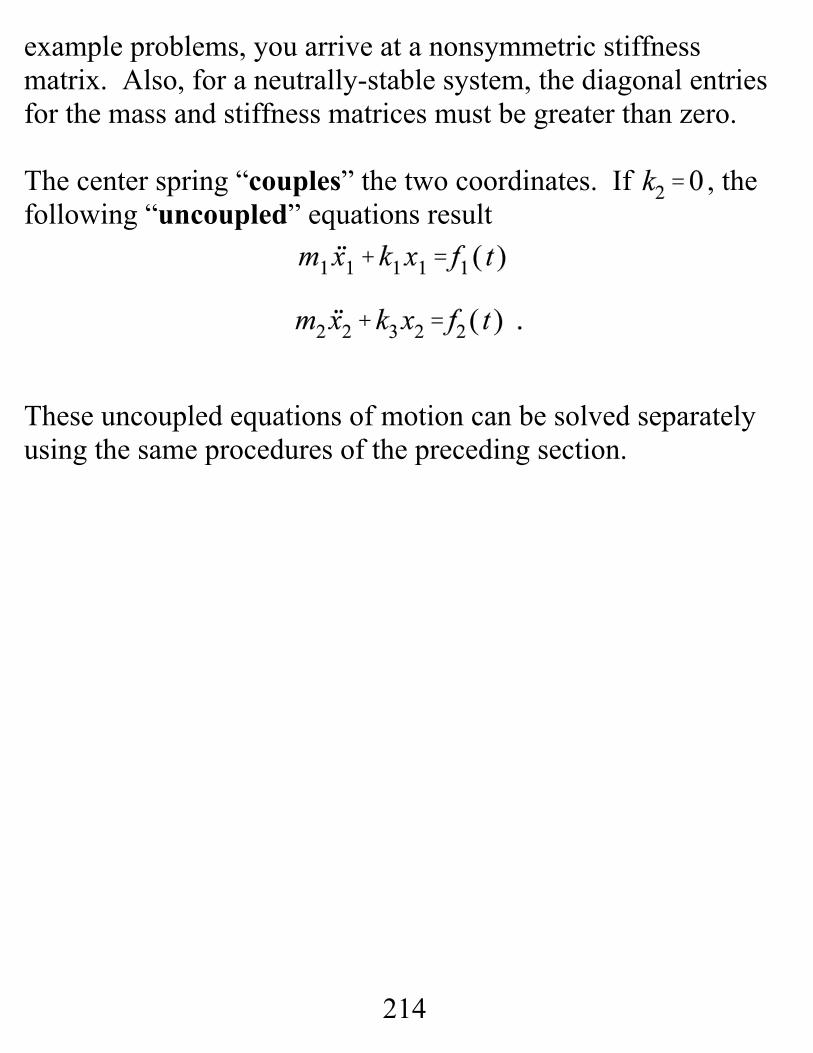
The center spring “couples” the two coordinates. If , thefollowing “uncoupled” equations result

These uncoupled equations of motion can be solved separatelyusing the same procedures of the preceding section.

215

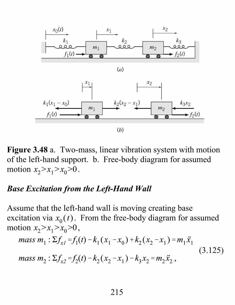
(3.125)

Figure 3.48 a. Two-mass, linear vibration system with motionof the left-hand support. b. Free-body diagram for assumedmotion .

Base Excitation from the Left-Hand Wall

Assume that the left-hand wall is moving creating base excitation via . From the free-body diagram for assumedmotion ,

216

(3.126)

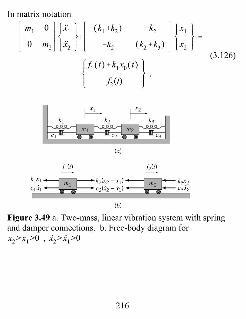
In matrix notation

Figure 3.49 a. Two-mass, linear vibration system with springand damper connections. b. Free-body diagram for

217

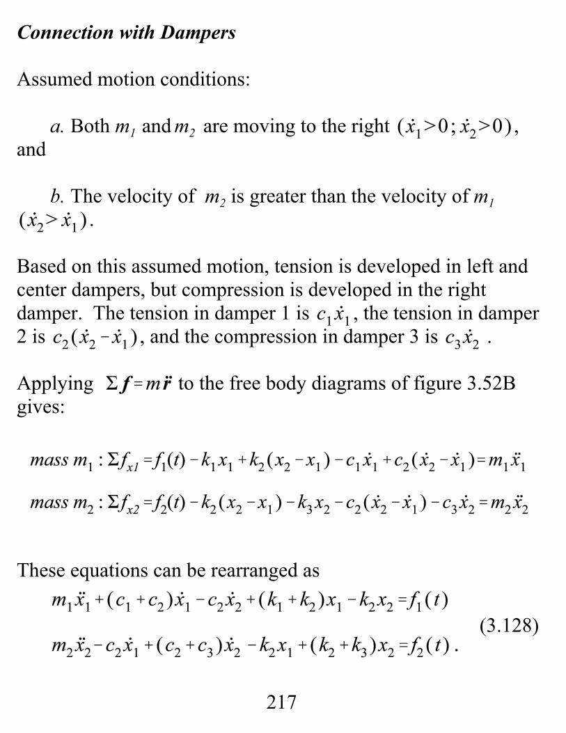
(3.128)

Connection with Dampers

Assumed motion conditions:

a. Both m1 and m2 are moving to the right ,and

b. The velocity of m2 is greater than the velocity of m1.

Based on this assumed motion, tension is developed in left andcenter dampers, but compression is developed in the rightdamper. The tension in damper 1 is , the tension in damper2 is , and the compression in damper 3 is .

Applying to the free body diagrams of figure 3.52Bgives:

These equations can be rearranged as

218

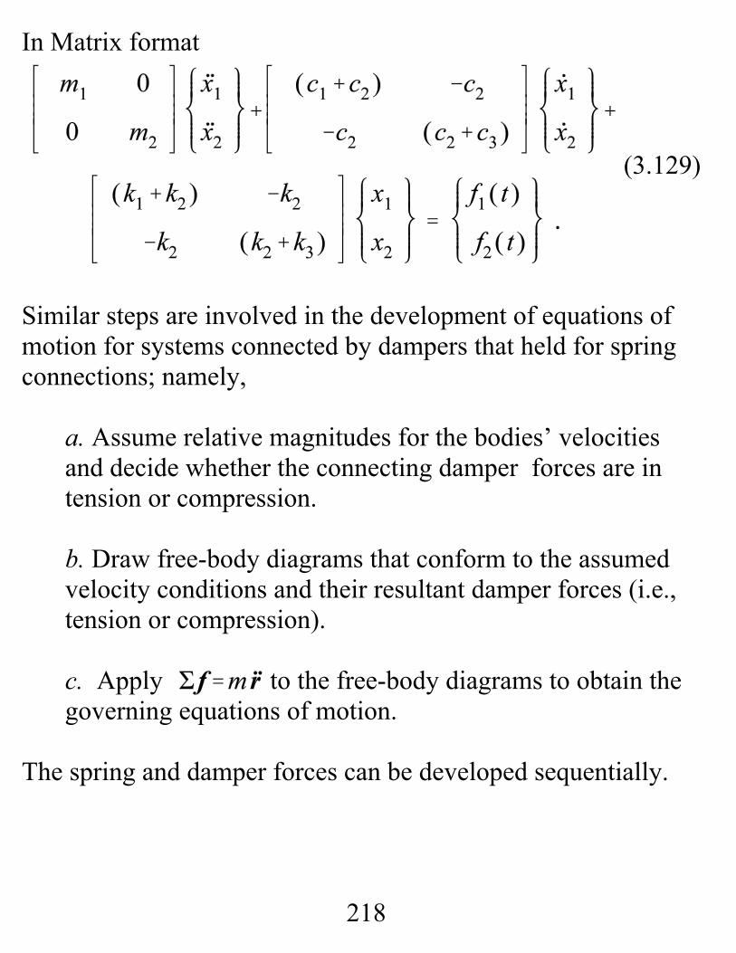
(3.129)

In Matrix format

Similar steps are involved in the development of equations ofmotion for systems connected by dampers that held for springconnections; namely,

a. Assume relative magnitudes for the bodies’ velocities and decide whether the connecting damper forces are intension or compression.

b. Draw free-body diagrams that conform to the assumedvelocity conditions and their resultant damper forces (i.e.,tension or compression).

c. Apply to the free-body diagrams to obtain thegoverning equations of motion.

The spring and damper forces can be developed sequentially.

219

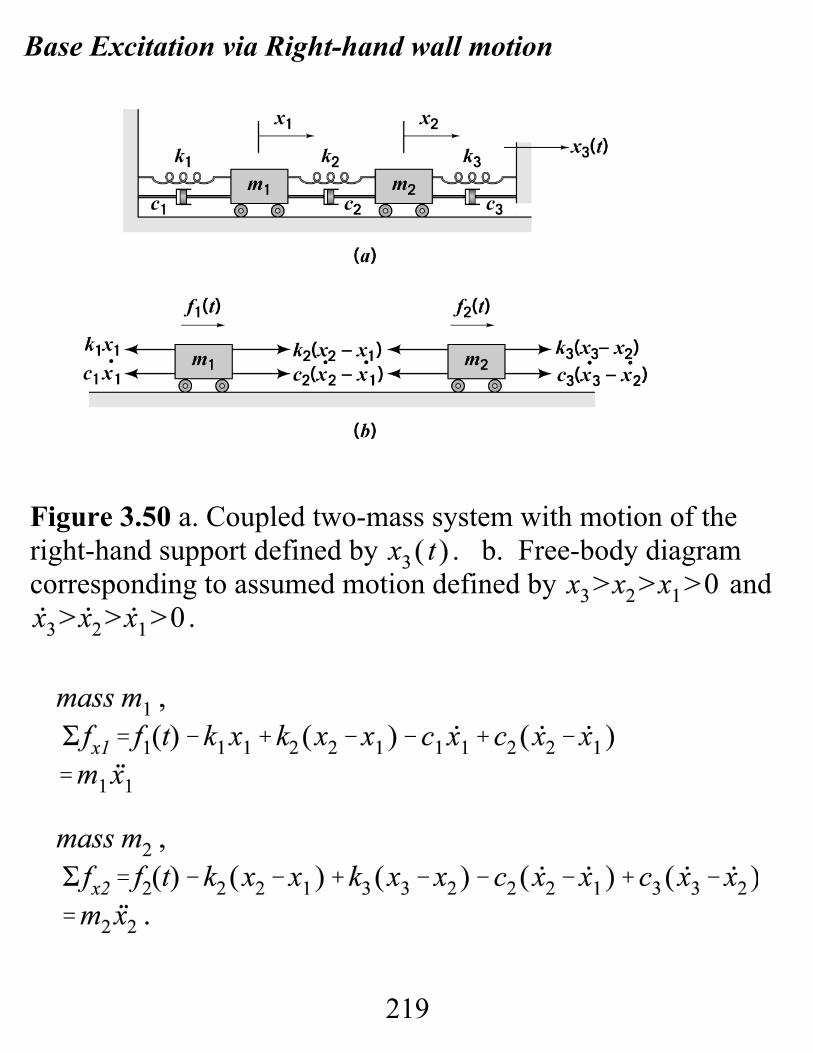
Base Excitation via Right-hand wall motion

Figure 3.50 a. Coupled two-mass system with motion of theright-hand support defined by . b. Free-body diagramcorresponding to assumed motion defined by and

.

220

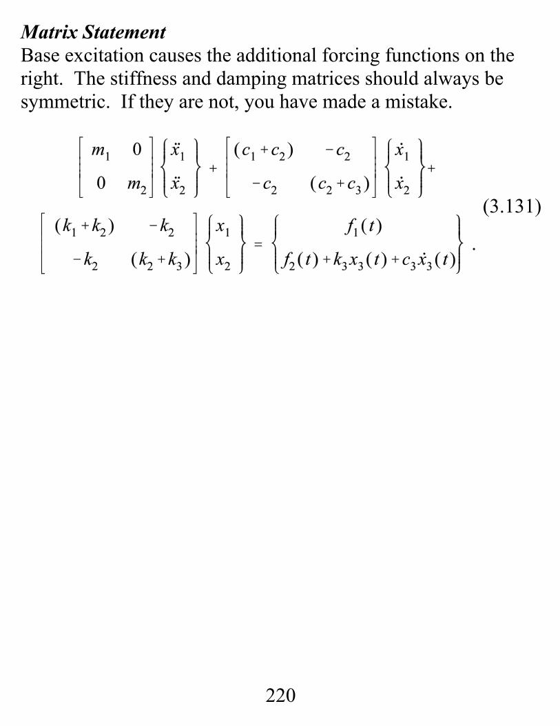
(3.131)

Matrix StatementBase excitation causes the additional forcing functions on theright. The stiffness and damping matrices should always besymmetric. If they are not, you have made a mistake.

221

(3.131)

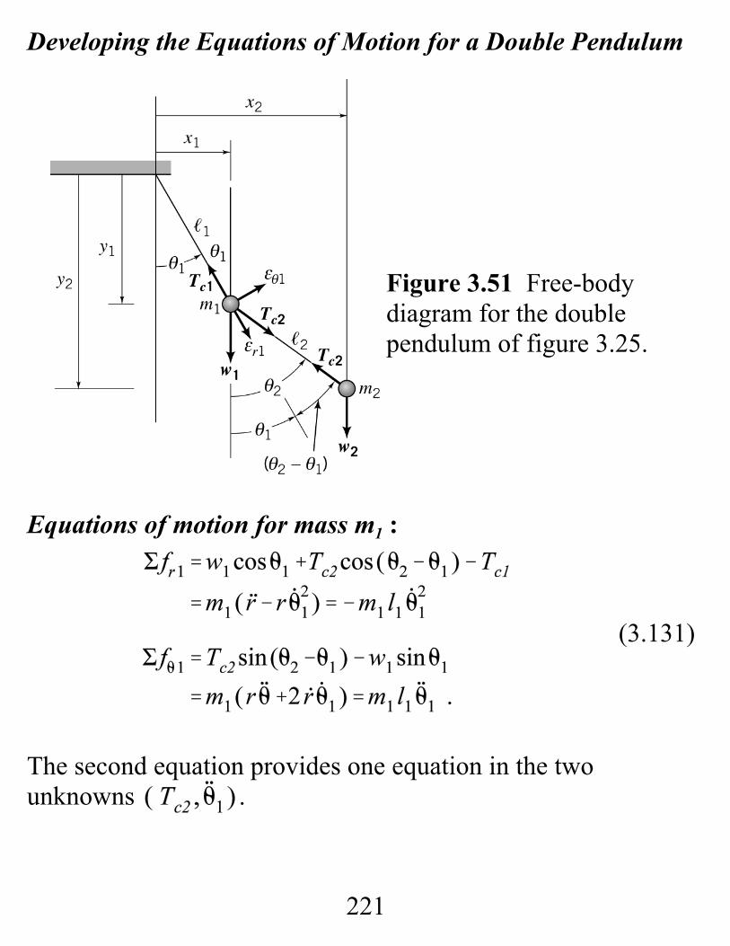
Developing the Equations of Motion for a Double Pendulum

Figure 3.51 Free-bodydiagram for the doublependulum of figure 3.25.

Equations of motion for mass m1 :

The second equation provides one equation in the twounknowns .

222

(3.82)

(3.132)

(3.133a)

(3.133b)

Simple -pendulum equations of motion,

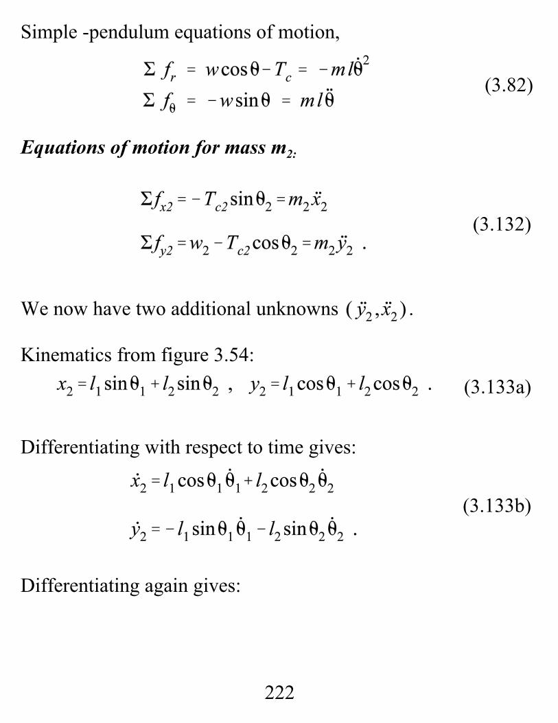
Equations of motion for mass m2:

We now have two additional unknowns .

Kinematics from figure 3.54:

Differentiating with respect to time gives:

Differentiating again gives:

223

(3.133c)

(3.134)

(3.135)

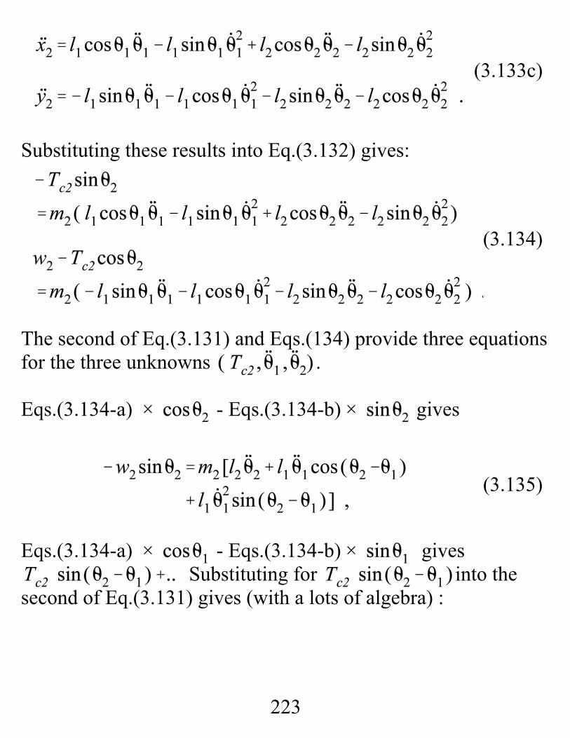
Substituting these results into Eq.(3.132) gives:

The second of Eq.(3.131) and Eqs.(134) provide three equationsfor the three unknowns .

Eqs.(3.134-a) - Eqs.(3.134-b) gives

Eqs.(3.134-a) - Eqs.(3.134-b) gives Substituting for into the

second of Eq.(3.131) gives (with a lots of algebra) :

224

(3.137)

This the second of the two required differential equations. Inmatrix format the model is

Note that this inertia matrix is neither diagonal nor symmetric,but it can be made symmetric; e.g., multiply the first equationby l1 and the second equation by l2. As with the stiffnessmatrix, the inertia matrix should be either symmetric, or capableof being made symmetric. Also, correct diagonal entries arepositive.

The linearized version of this equation is obtained by assumingthat both θ1 and θ2 are small (i.e., , etc.) and can be stated

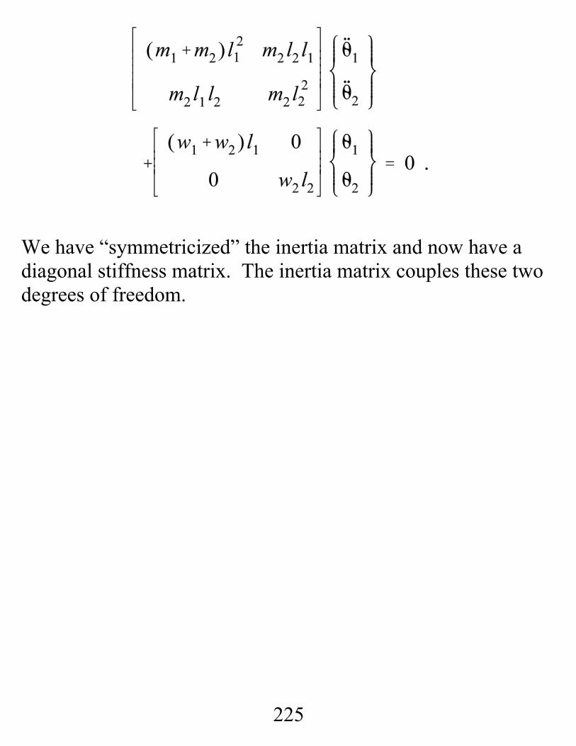
225

We have “symmetricized” the inertia matrix and now have adiagonal stiffness matrix. The inertia matrix couples these twodegrees of freedom.

226

(3.139)

(3.140)

Lecture 15. EIGENANALYSIS FOR 2DOF VIBRATIONEXAMPLES

Thinking about solving coupled linear differential equations byconsidering the problem of developing a solution to thefollowing homogeneous version of Eq.(3.124)

To find a solution to the one-degree-of-freedom problem, we “guessed” a solution of the form

. Substituting this guess netted

A nontrivial solution ( A … 0 ) requires that .

For Eq.(3.139) we will guess

Substituting this guessed solution gives

227

(3.141)

or

Solving for via Cramer’s rule gives:

where Δ is the determinant of the coefficient matrix. For anontrivial solution , Δ = 0; i.e., the coefficientmatrix must be singular.

228

(3.142)

(3.143)

(3.144)

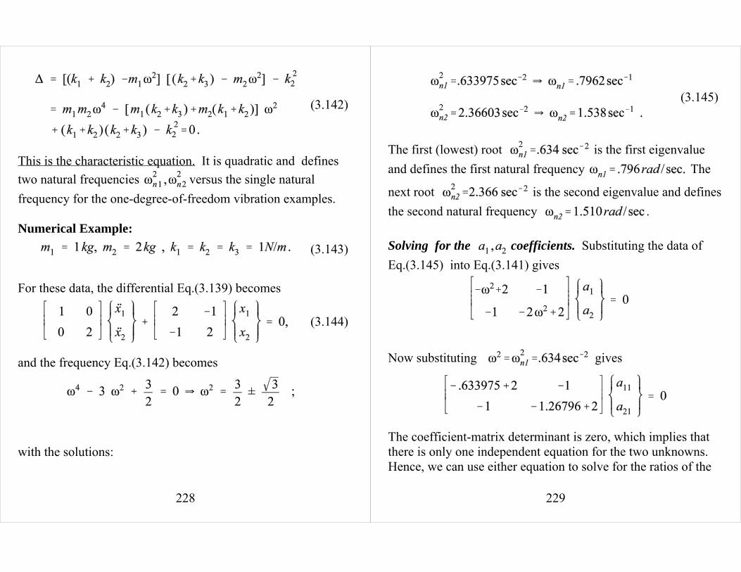
This is the characteristic equation. It is quadratic and definestwo natural frequencies versus the single naturalfrequency for the one-degree-of-freedom vibration examples.

Numerical Example:

For these data, the differential Eq.(3.139) becomes

and the frequency Eq.(3.142) becomes

with the solutions:

229

(3.145)

The first (lowest) root is the first eigenvalueand defines the first natural frequency The

next root is the second eigenvalue and definesthe second natural frequency . Solving for the coefficients. Substituting the data ofEq.(3.145) into Eq.(3.141) gives

Now substituting gives

The coefficient-matrix determinant is zero, which implies thatthere is only one independent equation for the two unknowns. Hence, we can use either equation to solve for the ratios of the

230

(3.147)

(3.146)

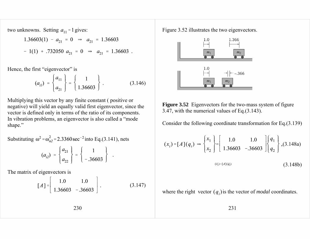
two unknowns. Setting gives:

Hence, the first “eigenvector” is

Multiplying this vector by any finite constant ( positive ornegative) will yield an equally valid first eigenvector, since thevector is defined only in terms of the ratio of its components. In vibration problems, an eigenvector is also called a “modeshape.”

Substituting into Eq.(3.141), nets

The matrix of eigenvectors is

231

(3.148a)

(3.148b)

Figure 3.52 illustrates the two eigenvectors.

Figure 3.52 Eigenvectors for the two-mass system of figure3.47, with the numerical values of Eq.(3.143).

Consider the following coordinate transformation for Eq.(3.139)

where the right vector is the vector of modal coordinates.

232

(3.150)

(3.149)

(3.148)

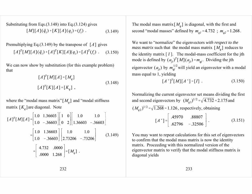
(3.149)Substituting from Eqs.(3.148) into Eq.(3.124) gives

Premultiplying Eq.(3.149) by the transpose of gives

We can now show by substitution (for this example problem)that

where the “modal mass matrix” and “modal stiffnessmatrix are diagonal. Note

233

(3.150)

(3.151)

The modal mass matrix is diagonal, with the first andsecond “modal masses” defined by .

We want to “normalize” the eigenvectors with respect to themass matrix such that the modal mass matrix reduces tothe identity matrix [ I ]. The modal-mass coefficient for the jthmode is defined by . Dividing the jth

eigenvector by will yield an eigenvector with a modalmass equal to 1, yielding

Normalizing the current eigenvector set means dividing the firstand second eigenvectors by and

, respectively, obtaining

You may want to repeat calculations for this set of eigenvectorsto confirm that the modal mass matrix is now the identitymatrix. Proceeding with this normalized version of theeigenvector matrix to verify that the modal stiffness matrix isdiagonal yields

234

(3.152)

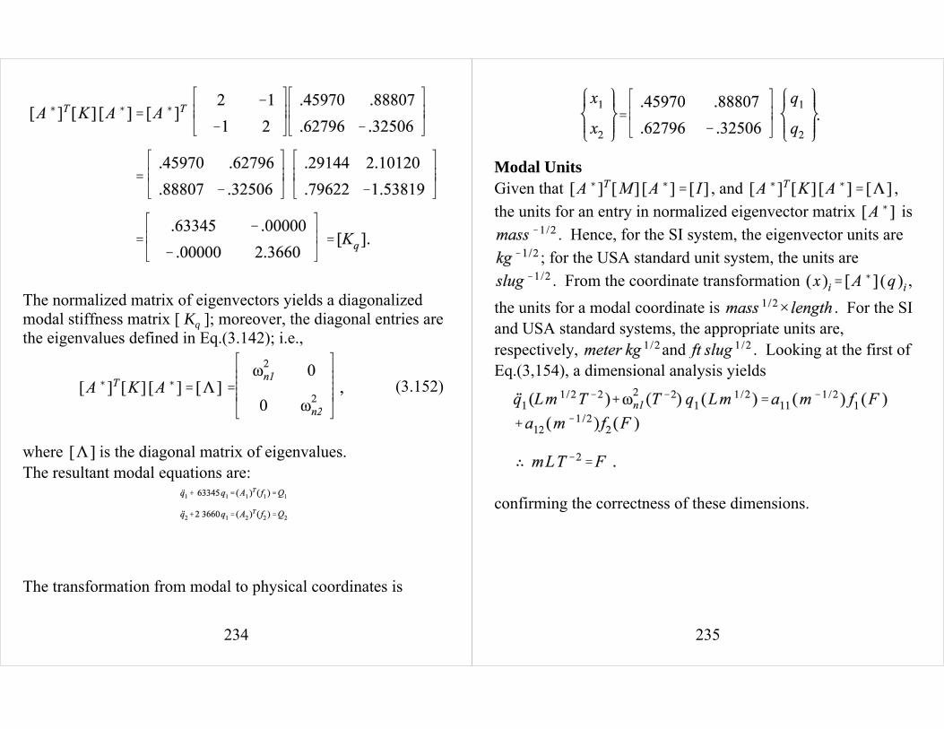
The normalized matrix of eigenvectors yields a diagonalizedmodal stiffness matrix [ Kq ]; moreover, the diagonal entries arethe eigenvalues defined in Eq.(3.142); i.e.,

where is the diagonal matrix of eigenvalues.The resultant modal equations are:

The transformation from modal to physical coordinates is

235

Modal UnitsGiven that , and ,the units for an entry in normalized eigenvector matrix is

. Hence, for the SI system, the eigenvector units are; for the USA standard unit system, the units are

. From the coordinate transformation ,the units for a modal coordinate is . For the SIand USA standard systems, the appropriate units are,respectively, and . Looking at the first ofEq.(3,154), a dimensional analysis yields

confirming the correctness of these dimensions.

236

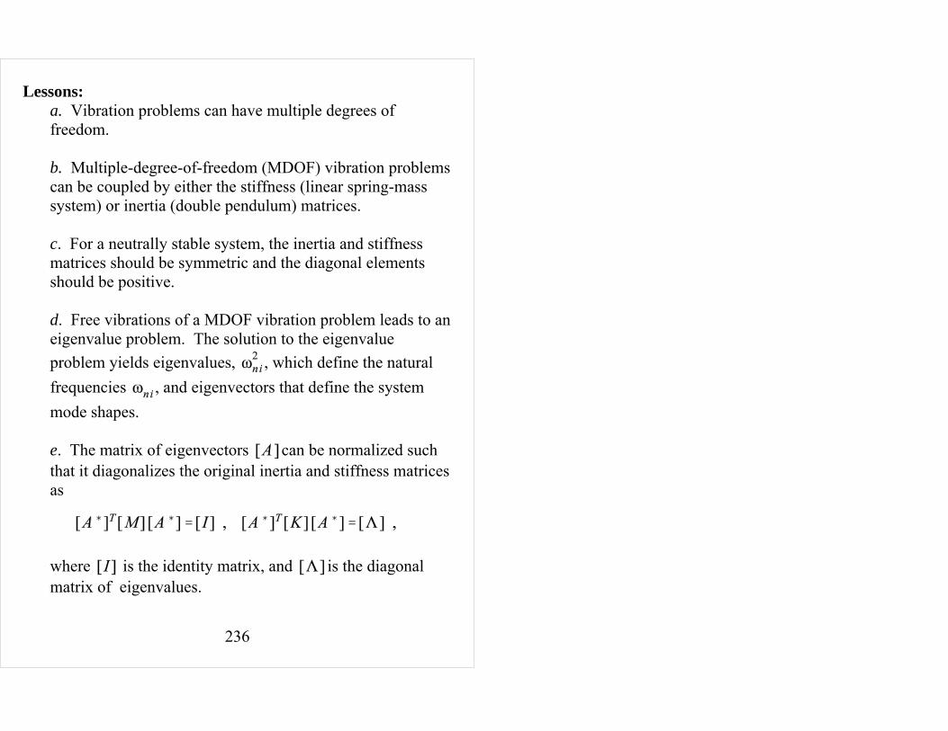
Lessons:a. Vibration problems can have multiple degrees offreedom.

b. Multiple-degree-of-freedom (MDOF) vibration problemscan be coupled by either the stiffness (linear spring-masssystem) or inertia (double pendulum) matrices.

c. For a neutrally stable system, the inertia and stiffnessmatrices should be symmetric and the diagonal elementsshould be positive.

d. Free vibrations of a MDOF vibration problem leads to aneigenvalue problem. The solution to the eigenvalueproblem yields eigenvalues, , which define the naturalfrequencies , and eigenvectors that define the systemmode shapes.

e. The matrix of eigenvectors can be normalized suchthat it diagonalizes the original inertia and stiffness matricesas

where is the identity matrix, and is the diagonalmatrix of eigenvalues.

237

(3.154)

(3.153)

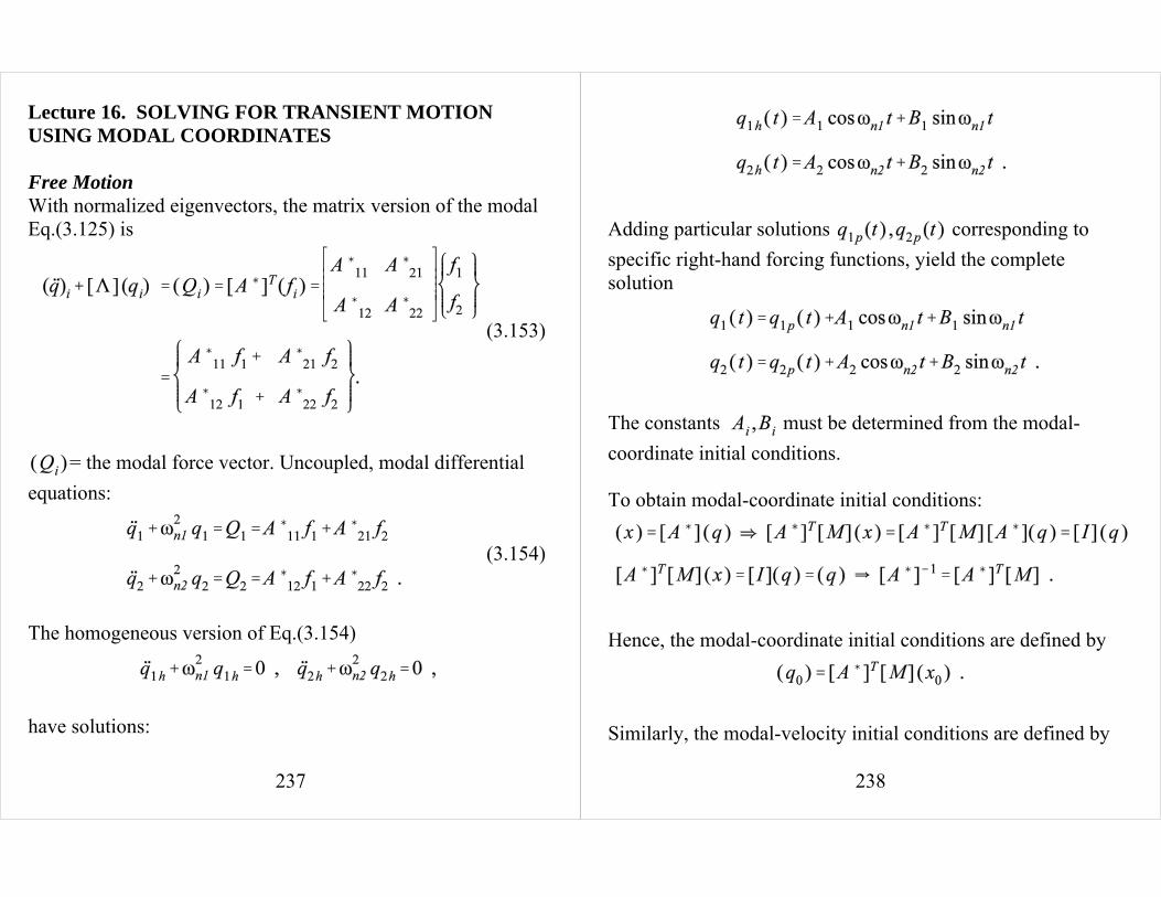
Lecture 16. SOLVING FOR TRANSIENT MOTIONUSING MODAL COORDINATES

Free MotionWith normalized eigenvectors, the matrix version of the modalEq.(3.125) is

= the modal force vector. Uncoupled, modal differentialequations:

The homogeneous version of Eq.(3.154)

have solutions:

238

Adding particular solutions corresponding tospecific right-hand forcing functions, yield the completesolution

The constants must be determined from the modal-coordinate initial conditions.

To obtain modal-coordinate initial conditions:

Hence, the modal-coordinate initial conditions are defined by

Similarly, the modal-velocity initial conditions are defined by

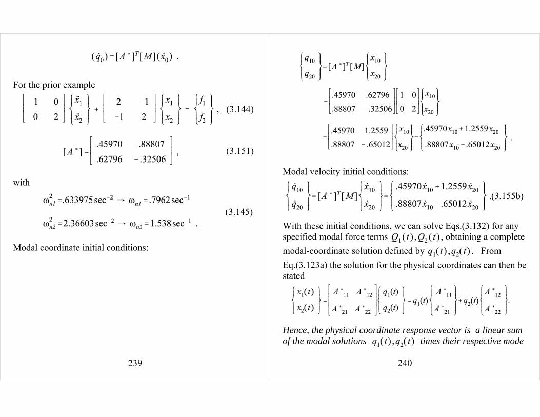
239

(3.144)

(3.145)

(3.151)

For the prior example

with

Modal coordinate initial conditions:

240

(3.155b)

Modal velocity initial conditions:

With these initial conditions, we can solve Eqs.(3.132) for anyspecified modal force terms , obtaining a completemodal-coordinate solution defined by . FromEq.(3.123a) the solution for the physical coordinates can then bestated

Hence, the physical coordinate response vector is a linear sumof the modal solutions times their respective mode

241

(3.157)

shapes (or eigenvectors).

Example. With , Eqs. (3.155)gives , and:

The corresponding physical-coordinate solution is

Any disturbance to the system from initial conditions (orexternal forces) will result in combined motion at the twonatural frequencies. Note that the physical initial conditions arecorrectly represented,

242

-1

-0.5

0

0.5

1

0 10 20 30 40

t

q_1

-1

-0.5

0

0.5

1

0 10 20 30 40

t

q_2

-2

-1

0

1

2

0 10 20 30 40

t

x_1

-1

-0.5

0

0.5

1

0 10 20 30 40

t

x_2

Figure 3.53 Solution from Eq.(3.157) for and for

243

( i )

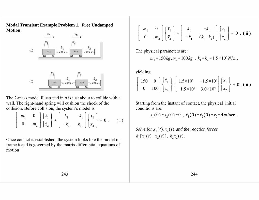
Modal Transient Example Problem 1. Free UndampedMotion

The 2-mass model illustrated in a is just about to collide with awall. The right-hand spring will cushion the shock of thecollision. Before collision, the system’s model is

Once contact is established, the system looks like the model offrame b and is governed by the matrix differential equations ofmotion

244

( ii )

( ii )

The physical parameters are:

yielding

Starting from the instant of contact, the physical initialconditions are:

Solve for and the reaction forces

.

245

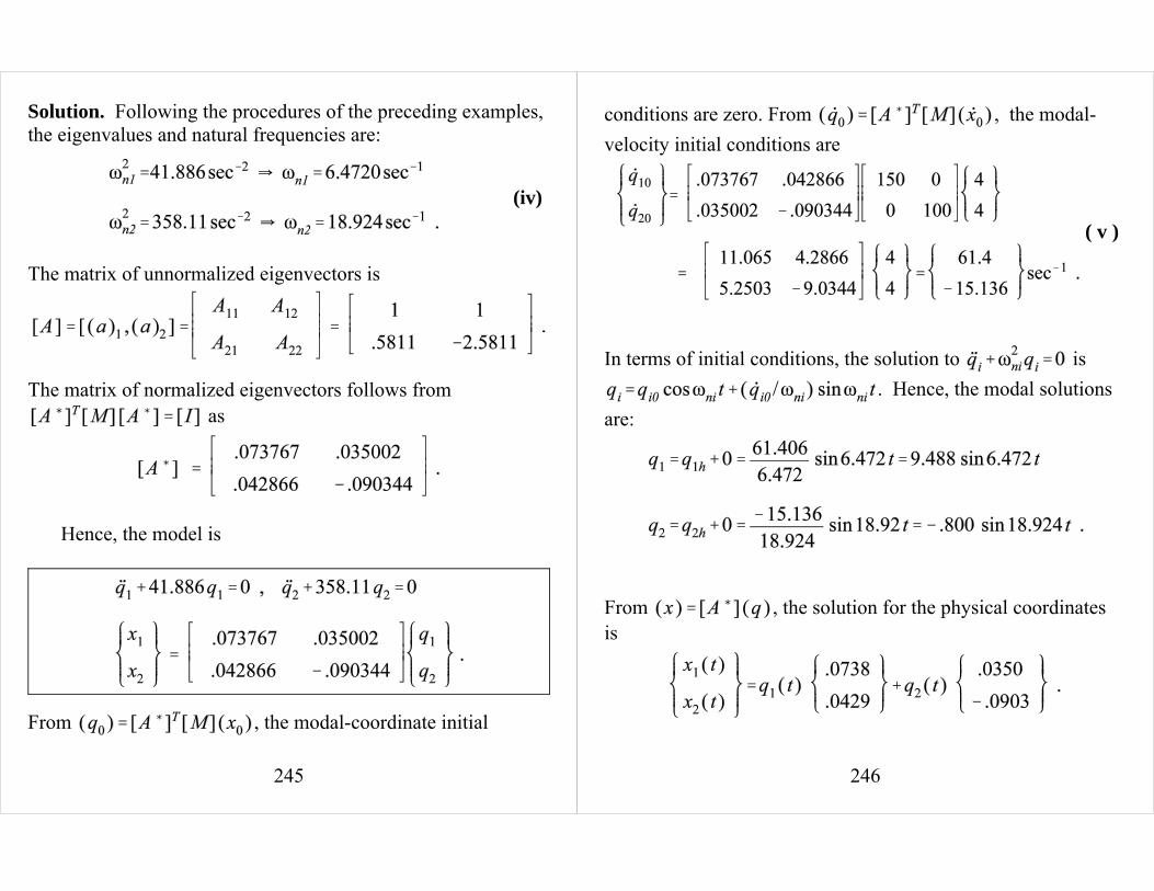
(iv)

Solution. Following the procedures of the preceding examples,the eigenvalues and natural frequencies are:

The matrix of unnormalized eigenvectors is

The matrix of normalized eigenvectors follows from as

Hence, the model is

From , the modal-coordinate initial

246

( v )

conditions are zero. From , the modal-velocity initial conditions are

In terms of initial conditions, the solution to is. Hence, the modal solutions

are:

From , the solution for the physical coordinates is

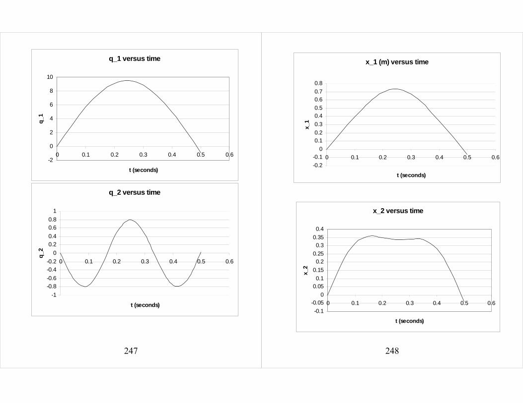
247

q_2 versus time

-1

-0.8-0.6

-0.4-0.2

0

0.20.4

0.60.8

1

0 0.1 0.2 0.3 0.4 0.5 0.6

t (seconds)

q_2

q_1 versus time

-2

0

2

4

6

8

10

0 0.1 0.2 0.3 0.4 0.5 0.6

t (seconds)

q_1

248

x_1 (m) versus time

-0.2

-0.10

0.10.2

0.3

0.40.5

0.60.7

0.8

0 0.1 0.2 0.3 0.4 0.5 0.6

t (seconds)

x_1

x_2 versus time

-0.1

-0.050

0.050.1

0.15

0.20.25

0.30.35

0.4

0 0.1 0.2 0.3 0.4 0.5 0.6

t (seconds)

x_2

249

f_s1=k_1 (x_1 - x_2 ) versus time

-1000

0

1000

2000

3000

4000

5000

6000

7000

0 0.1 0.2 0.3 0.4 0.5 0.6

t (seconds)

f_s1

= k

_1 (

x_1

- x_

2 )

(N)

f_s2 = k_2 x_2 versus time

-1000

0

1000

2000

3000

4000

5000

6000

0 0.1 0.2 0.3 0.4 0.5 0.6

time (seconds)

f_s2

= k

_2 x

_2 (

N)

250

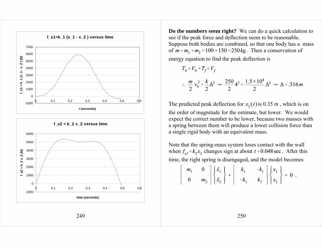
Do the numbers seem right? We can do a quick calculation tosee if the peak force and deflection seem to be reasonable. Suppose both bodies are combined, so that one body has a massof . Then a conservation ofenergy equation to find the peak deflection is

The predicted peak deflection for is 0.35 m , which is onthe order of magnitude for the estimate, but lower. We wouldexpect the correct number to be lower, because two masses witha spring between them will produce a lower collision force thana single rigid body with an equivalent mass.

Note that the spring-mass system loses contact with the wallwhen changes sign at about . After thistime, the right spring is disengaged, and the model becomes

251

(3.23)

(3.24)

(3.25)

Damping and Modal Damping FactorsThe SDOF harmonic oscillator equation of motion is

yields the homogeneous equation

Assumed solution: Yh=Aest yields:

Since A … 0, and ,

For ζ<1, the roots are

is called the damped natural frequency. Thehomogeneous solution looks like

252

where A1 and A2 are complex coefficients. The solution can bestated

where A and B are real constants.

MDOF vibration problems with general damping matricesmodeled by,

also have complex roots (eigenvalues) and eigenvectors.

The matrix of real eigenvectors, based on a symmetric stiffness and mass matrices, will only diagonalize a damping

matrix that can be stated as a linear summation of and; i.e.,

For a damping matrix of this particular (and very unlikely)form, the modal damping matrix is defined by

253

where and are the identity matrix and the diagonalmatrix of eigenvectors, respectively. With this damping-matrixformat, an n-degree-of-freedom vibration problem will havemodal differential equations of the form:

This is not a very useful or generally applicable result. Forlightly damped systems, damping is more often introduceddirectly in the undamped modal equations via :

The damping factors are specified for each modaldifferential equation, based on measurements or experience.

254

(3.129)

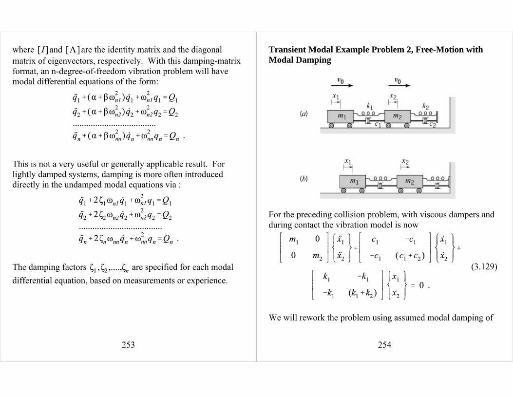
Transient Modal Example Problem 2, Free-Motion withModal Damping

For the preceding collision problem, with viscous dampers andduring contact the vibration model is now

We will rework the problem using assumed modal damping of

255

(3.27)

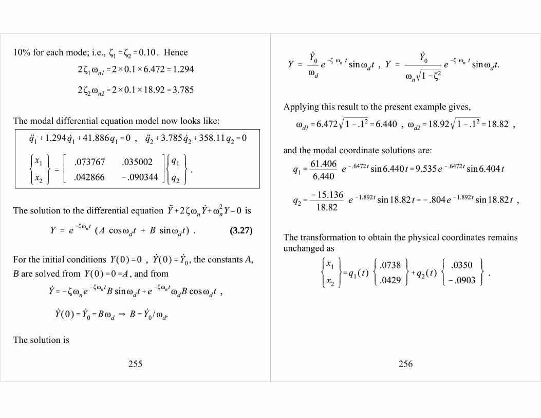
10% for each mode; i.e., . Hence

The modal differential equation model now looks like:

The solution to the differential equation is

For the initial conditions , the constants A,B are solved from , and from

The solution is

256

Applying this result to the present example gives,

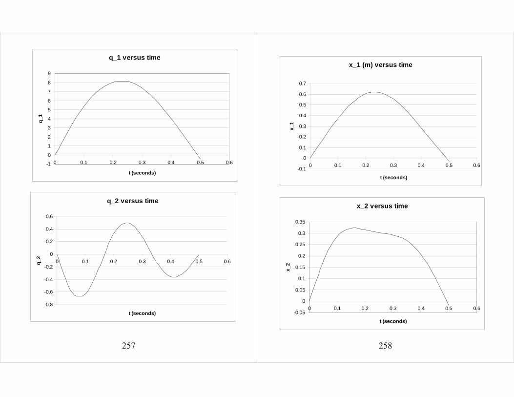
and the modal coordinate solutions are:

The transformation to obtain the physical coordinates remainsunchanged as

257

q_1 versus time

-1

0

1

2

3

4

5

6

7

8

9

0 0.1 0.2 0.3 0.4 0.5 0.6

t (seconds)

q_1

q_2 versus time

-0.8

-0.6

-0.4

-0.2

0

0.2

0.4

0.6

0 0.1 0.2 0.3 0.4 0.5 0.6

t (seconds)

q_2

258

x_1 (m) versus time

-0.1

0

0.1

0.2

0.3

0.4

0.5

0.6

0.7

0 0.1 0.2 0.3 0.4 0.5 0.6

t (seconds)

x_1

x_2 versus time

-0.05

0

0.05

0.1

0.15

0.2

0.25

0.3

0.35

0 0.1 0.2 0.3 0.4 0.5 0.6

t (seconds)

x_2

259

f_s1 = k_1 (x_1 - x_2) versus time

-1000

0

1000

2000

3000

4000

5000

0 0.1 0.2 0.3 0.4 0.5 0.6

t (seconds)

f_s1

= k

_1 (

x_1

- x

_2)

(N)

f_s2 = k_2 x_2 versus time

-1000

0

1000

2000

3000

4000

5000

6000

0 0.1 0.2 0.3 0.4 0.5 0.6

t (seconds)

f_s2

= k

_2 x

_2 (

N)

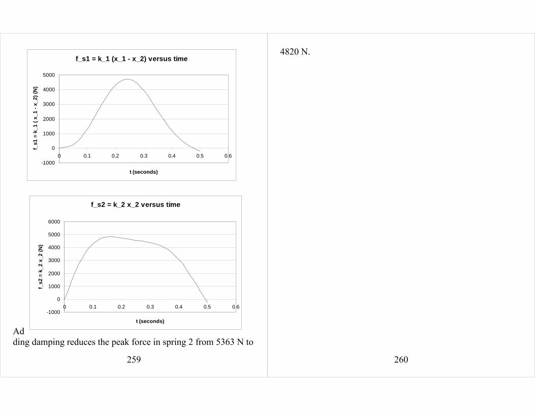
Adding damping reduces the peak force in spring 2 from 5363 N to

260

4820 N.

261

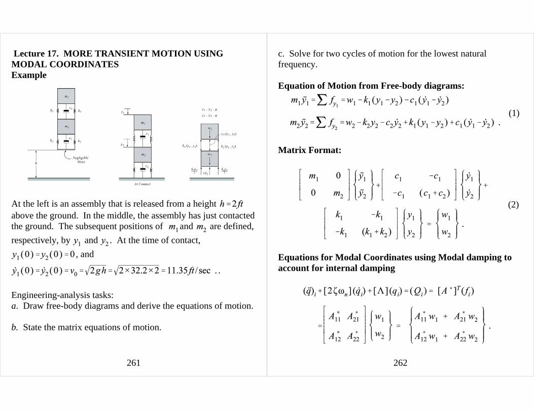
Lecture 17. MORE TRANSIENT MOTION USINGMODAL COORDINATESExample

At the left is an assembly that is released from a height above the ground. In the middle, the assembly has just contactedthe ground. The subsequent positions of and are defined,

respectively, by and . At the time of contact,

, and

.

Engineering-analysis tasks:a. Draw free-body diagrams and derive the equations of motion.

b. State the matrix equations of motion.

262

(2)

c. Solve for two cycles of motion for the lowest naturalfrequency.

Equation of Motion from Free-body diagrams:

Matrix Format:

Equations for Modal Coordinates using Modal damping toaccount for internal damping

(1)

263

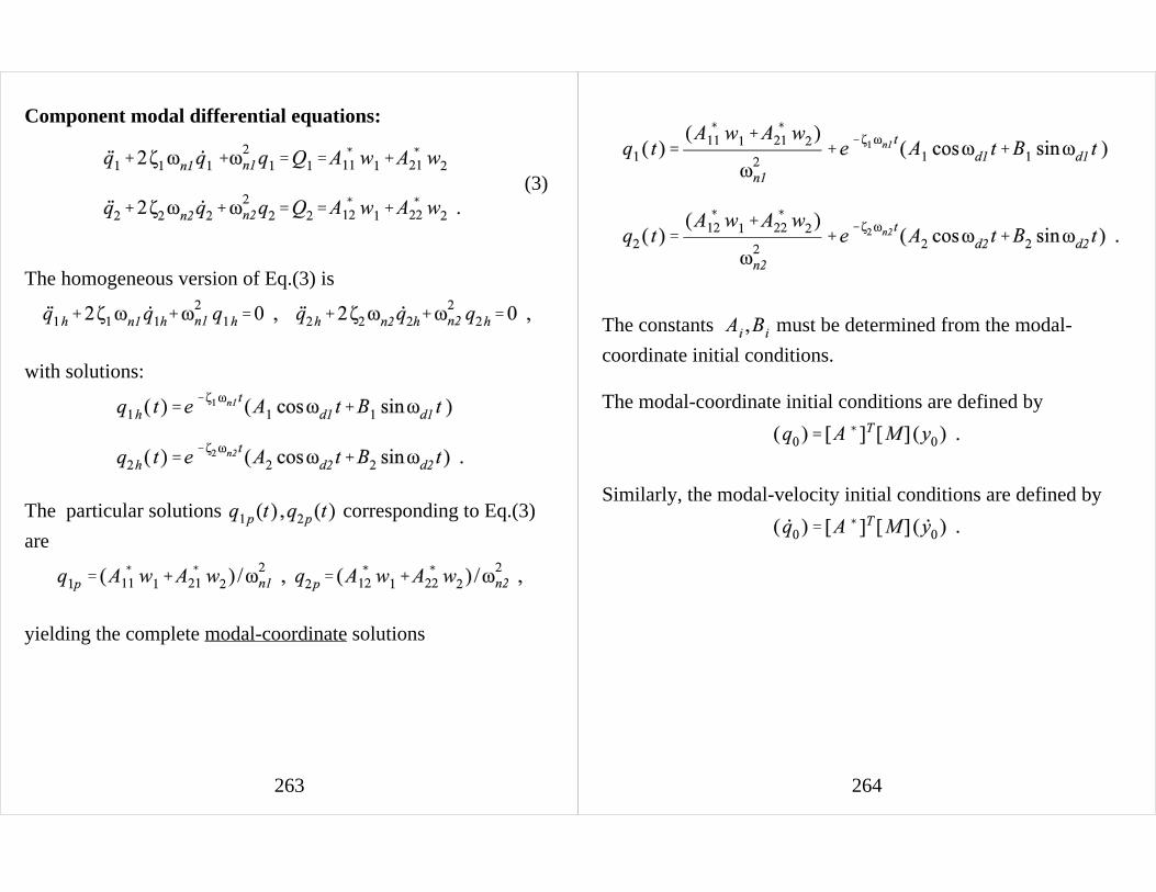
(3)

Component modal differential equations:

The homogeneous version of Eq.(3) is

with solutions:

The particular solutions corresponding to Eq.(3)

are

yielding the complete modal-coordinate solutions

264

The constants must be determined from the modal-

coordinate initial conditions.

The modal-coordinate initial conditions are defined by

Similarly, the modal-velocity initial conditions are defined by

265

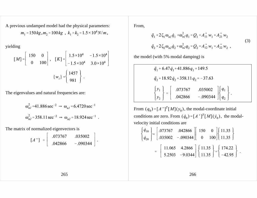
A previous undamped model had the physical parameters:

yielding

The eigenvalues and natural frequencies are:

The matrix of normalized eigenvectors is

266

(3)

From,

the model (with 5% modal damping) is

From , the modal-coordinate initial

conditions are zero. From , the modal-

velocity initial conditions are

267

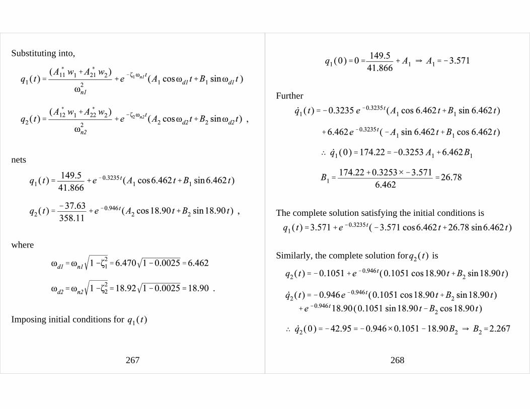
Substituting into,

nets

where

Imposing initial conditions for

268

Further

The complete solution satisfying the initial conditions is

Similarly, the complete solution for is

269

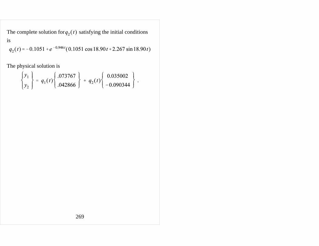
The complete solution for satisfying the initial conditions

is

The physical solution is

270

(3.158)

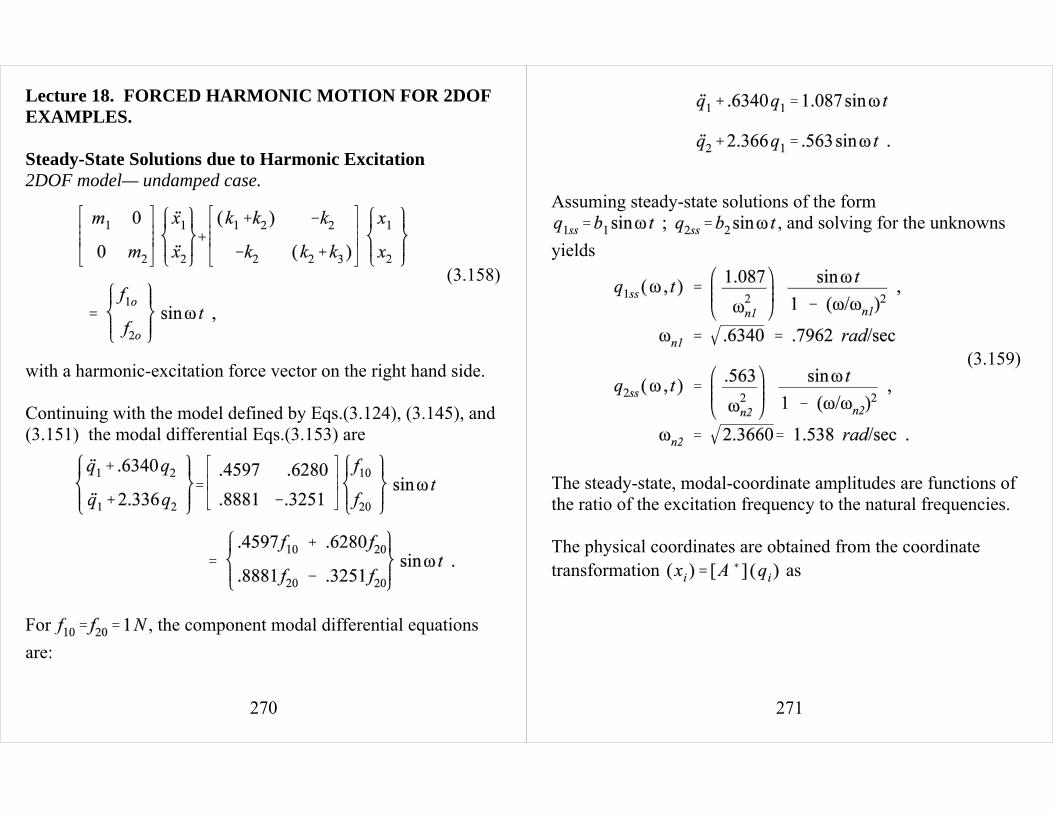
Lecture 18. FORCED HARMONIC MOTION FOR 2DOFEXAMPLES.

Steady-State Solutions due to Harmonic Excitation2DOF model— undamped case.

with a harmonic-excitation force vector on the right hand side.

Continuing with the model defined by Eqs.(3.124), (3.145), and(3.151) the modal differential Eqs.(3.153) are

For , the component modal differential equationsare:

271

(3.159)

Assuming steady-state solutions of the form, and solving for the unknowns

yields

The steady-state, modal-coordinate amplitudes are functions ofthe ratio of the excitation frequency to the natural frequencies.

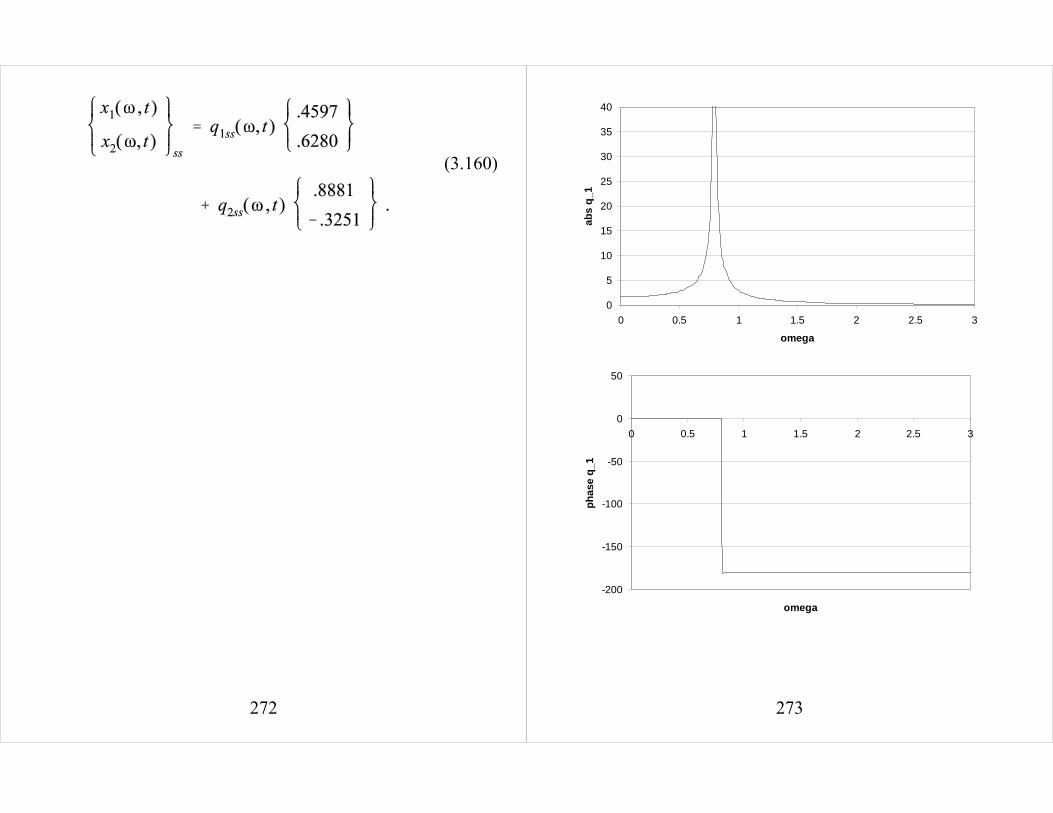
The physical coordinates are obtained from the coordinatetransformation as

272

(3.160)

273

0

5

10

15

20

25

30

35

40

0 0.5 1 1.5 2 2.5 3

omega

abs

q_1

-200

-150

-100

-50

0

50

0 0.5 1 1.5 2 2.5 3

omega

ph

ase

q_1

274

0

5

10

15

20

25

30

0 0.5 1 1.5 2 2.5 3

omega

abs

q_2

-200

-150

-100

-50

0

50

0 0.5 1 1.5 2 2.5 3

omega

ph

ase

q_2

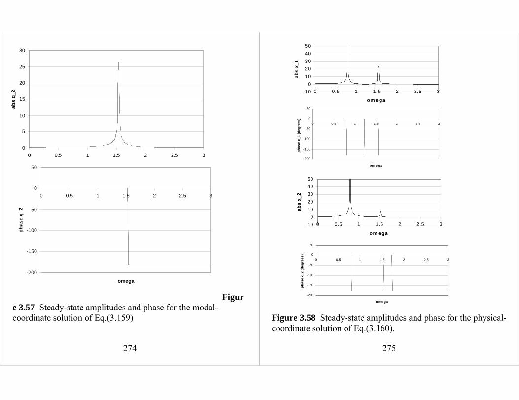
Figure 3.57 Steady-state amplitudes and phase for the modal-coordinate solution of Eq.(3.159)

275

-10

0

10

20

30

40

50

0 0.5 1 1.5 2 2.5 3

om e ga

ab

s x

_1

-200

-150

-100

-50

0

50

0 0.5 1 1.5 2 2.5 3

omega

ph

ase

x_1

(deg

rees

)

-10

0

10

20

30

40

50

0 0.5 1 1.5 2 2.5 3

om e ga

ab

s x

_2

-200

-150

-100

-50

0

50

0 0.5 1 1.5 2 2.5 3

omegap

has

e x_

2 (d

egre

es)

Figure 3.58 Steady-state amplitudes and phase for the physical-coordinate solution of Eq.(3.160).

276

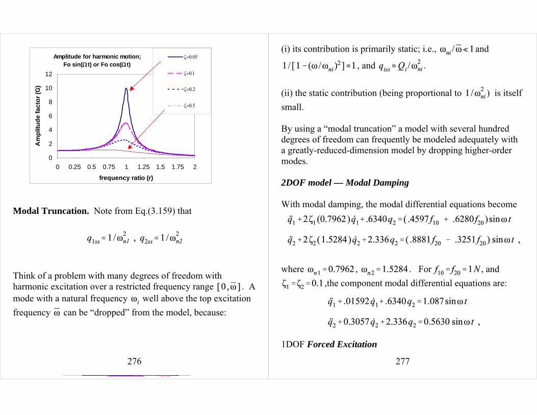
Amplitude for harmonic motion;Fo sin(Ωt) or Fo cos(Ωt)

0

2

4

6

8

10

12

0 0.25 0.5 0.75 1 1.25 1.5 1.75 2

frequency ratio (r)

Am

plit

ud

e f

ac

tor

(G)

ζ=0.05

ζ=0.1

ζ=0.2

ζ=0.5

1 2

Modal Truncation. Note from Eq.(3.159) that

Think of a problem with many degrees of freedom withharmonic excitation over a restricted frequency range . Amode with a natural frequency well above the top excitationfrequency can be “dropped” from the model, because:

277

(i) its contribution is primarily static; i.e., and

, and .

(ii) the static contribution (being proportional to ) is itselfsmall. By using a “modal truncation” a model with several hundreddegrees of freedom can frequently be modeled adequately witha greatly-reduced-dimension model by dropping higher-ordermodes.

2DOF model — Modal Damping

With modal damping, the modal differential equations become

where , . For , and,the component modal differential equations are:

1DOF Forced Excitation

278

(3.32)

(3.33)

(3.38)

(3.36)

Dividing through by the mass m gives

The steady-solution defined can be restated

where Yop is the amplitude of the solution, and ψ is the phasebetween the solution Yp( t ) and the input excitation force

. The solution for Yop is

where

Note that Eq.(3.38) can be stated

279

(3.38a)

(3.39)

The phase is

280

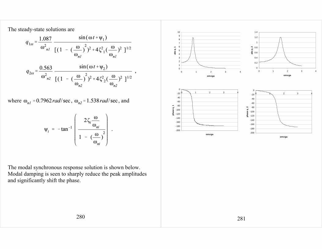
The steady-state solutions are

where , , and

The modal synchronous response solution is shown below. Modal damping is seen to sharply reduce the peak amplitudesand significantly shift the phase.

281

0

1

2

3

4

5

6

7

8

9

10

0 1 2 3 4

omega

ab

s q

_1

-200

-180

-160

-140

-120

-100

-80

-60

-40

-20

0

0 1 2 3 4

omega

ph

as

e q

_2

-200

-180

-160

-140

-120

-100

-80

-60

-40

-20

0

0 1 2 3 4

omega

ph

ase

q_1

0

0.2

0.4

0.6

0.8

1

1.2

1.4

0 1 2 3 4

omega

abs

q_2

282

0

0.5

1

1.5

2

2.5

3

3.5

4

4.5

0 0.5 1 1.5 2 2.5 3 3.5

omega

abs

x_1

-1

0

1

2

3

4

5

6

0 0.5 1 1.5 2 2.5 3 3.5

omega

abs

x_2

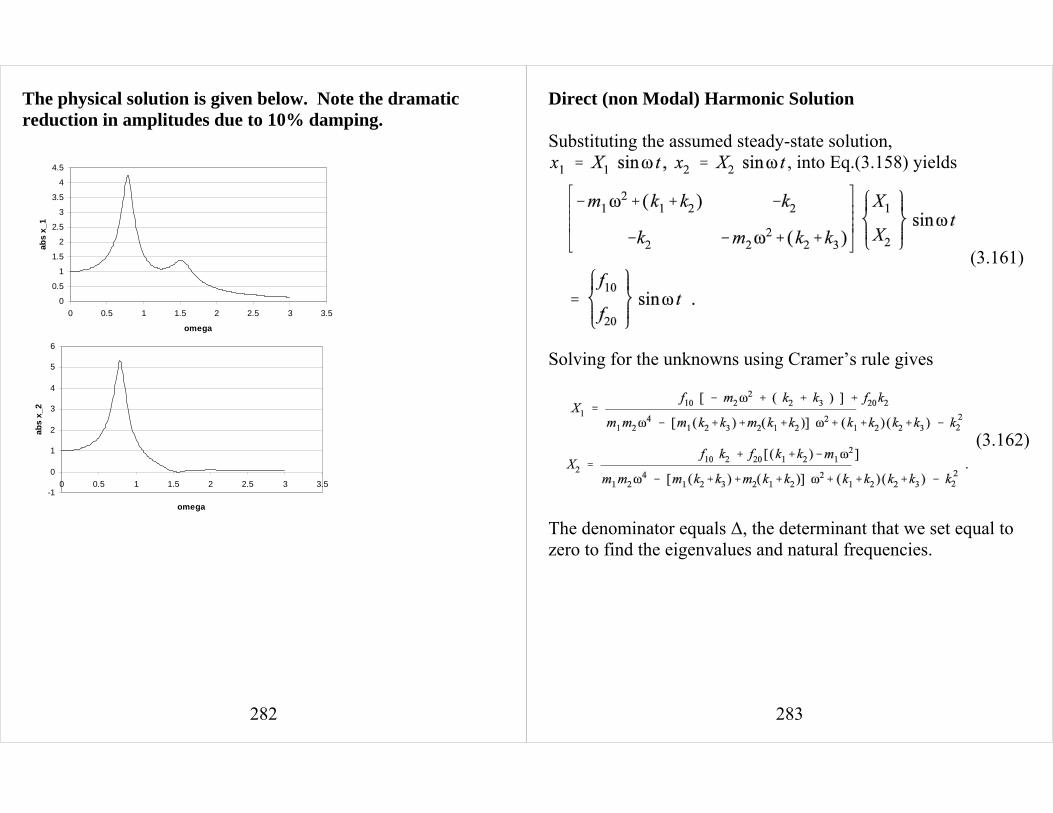
The physical solution is given below. Note the dramaticreduction in amplitudes due to 10% damping.

283

(3.161)

(3.162)

Direct (non Modal) Harmonic Solution

Substituting the assumed steady-state solution,, into Eq.(3.158) yields

Solving for the unknowns using Cramer’s rule gives

The denominator equals Δ, the determinant that we set equal tozero to find the eigenvalues and natural frequencies.

284

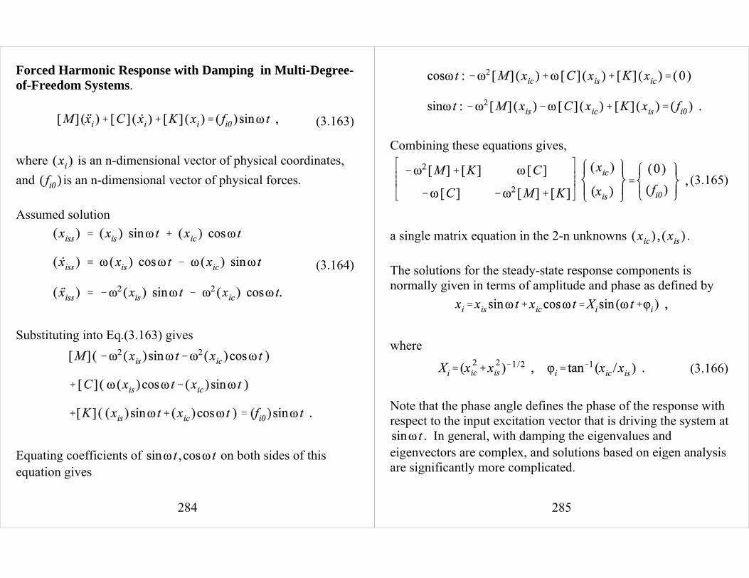
(3.163)

(3.164)

Forced Harmonic Response with Damping in Multi-Degree-of-Freedom Systems.

where is an n-dimensional vector of physical coordinates,and is an n-dimensional vector of physical forces.

Assumed solution

Substituting into Eq.(3.163) gives

Equating coefficients of on both sides of thisequation gives

285

(3.166)

(3.165)

Combining these equations gives,

a single matrix equation in the 2-n unknowns .

The solutions for the steady-state response components isnormally given in terms of amplitude and phase as defined by

where

Note that the phase angle defines the phase of the response withrespect to the input excitation vector that is driving the system at

. In general, with damping the eigenvalues andeigenvectors are complex, and solutions based on eigen analysisare significantly more complicated.

286

Lessons

a. For undamped systems with symmetric mass andstiffness matrices, the eigenvalues and eigenvectors arereal.

b. The matrix of real eigenvectors can be used touncouple the symmetric stiffness and mass matrices yieldinguncoupled modal differential equations.

c. The matrix of eigenvectors can be normalized such that and .

d. Modal coordinate and velocity initial conditions can becalculated from the transformation as

and .

e. For free motion, the physical solution consists of asummation of the modal solutions times their eigenvectors.

f. With harmonic excitation, the physical solution consists ofa summation of the modal solutions times their eigenvectors.

g. Harmonic solutions can be directly calculated forvibration systems defined by symmetric stiffness and massmatrices and general damping matrices. The solution isobtained in terms of amplitudes and phase values at each

287

excitation frequency.