Lecture 13, 14: Routing Algorithms ELEN E6761: Communication Networks Instructor: Javad Ghaderi...

Lecture 13, 14: Routing Algorithms

ELEN E6761:Communication Networks

Instructor: Javad Ghaderi

Slides adapted from “Computer Networking: A Top Down Approach” Jim Kurose, Keith Ross

Network Layer and Routing Algorithms Introduction What’s inside a router The network layer Protocols Routing algorithms

Some graph definitions Link State Distance Vector

Routing in the Internet Broadcast and multicast routing

Network layer transport segment from source to destination host on source side encapsulates segments into datagrams on destination side, delivers segments to transport layer network layer protocols in every host and router router examines header fields in all IP datagrams

passing through it

Packets in differentlayers have different names(Recall encapsulation in Lecture 1)

application

transportnetworkdata linkphysical

application


networkdata linkphysical network

data linkphysical

networkdata linkphysical







networkdata linkphysicalnetwork

data linkphysical

Connectionless Routing Postal service abstraction (Internet)

Model• no call setup or teardown at network layer• no service guarantees

Network support• no state within network on end-to-end connections• packets forwarded based on destination host ID• packets between same source-dest pair may take

different paths

application


application


1. Send data 2. Receive data

Network Layer and Routing Algorithms Introduction What’s inside a router? The network layer Protocols Routing algorithms



Router ArchitectureTwo key router functions: Routing

Determine route taken by packets from source to destination

Run routing algorithms and generate lookup (forwarding) tables

Switching Process of moving packets from input port to output

port Lookup forwarding table given information in packet Switch/forward packets from incoming to outgoing

link based on route

Router Architecture Switch + Lookup (forwarding) table

SwitchingFabric

queueLookupqueueLookup

queueLookup

Input link 1Input link 2

Input link N

Output link 1

Output link 2

Output link N

Packet arrives at input link The lookup table determines the corresponding

output link based on the packet header (packet destination)

Packet is transferred to the corresponding output link using switch

Network Layer and Routing Algorithms Introduction What’s inside a router The network layer protocols Routing algorithms



The Internet Network layer

forwardingtable

Host, router network layer functions:

Routing protocols•path selection

IP protocol•addressing conventions•datagram format•packet handling conventions

Transport layer: TCP, UDP

Link layer

physical layer

Networklayer

IP datagram format

miscellaneousfields

sourceIP address

destinationIP address data

Miscellaneous fields: • Protocol version• Total header length• Total datagram length• TTL (time to live)• …

datagram remains unchanged, as it travels from source to destination

Network Layer and Routing Algorithms Introduction What’s inside a router The network layer protocols Routing algorithms



1

23

0111

Destination IP address in arrivingpacket’s header

routing algorithm

local forwarding tableheader value output link

0100010101111001

3221

Interplay between routing, forwarding Previous Lectures:

Forward (switch algorithms) assuming forwarding table is known

Q: How to generate forwarding tables? Routing algorithms

and protocols

Routing based on dest IP address Hop-by-hop forwarding based on destination

IP carried by packet Each packet has destination IP address Each router has forwarding table of..

• destination IP next hop IP address IP route table calculated in network routers

Most prevalent way to route on the Internet Distributed routing algorithm for calculating

forwarding tables

Routing Example

Receiver

Packet R

Sender

2

34

1

2

34

1

2

34

1

R2

R3

R1

R

RR 3

R 4

R 3

R

Routing based on dest Address Advantages

Totally distributed Disadvantages

Every router knows about every destination• Potentially large tables

All packets to destination take same route

Routing protocols

Graph abstraction for routing algorithms:

Graph: G = (N,E) N=graph nodes (routers)

• A, B, C, D, E, F E=graph edges (links)

• (A,B), (A,D), (A,C), (B,C), (B,D), (C,D), (C,E), (C,F), (D,E), (E,F)

• Cost associated with edge– Delay, $, congestion

Routing algorithms find minimum cost paths through graph

Goal: determine “good” path (sequence of routers) thru network from source to dest.

A

ED

CB

F2

21

3

1

12

53

5

Routing Algorithms

Global or decentralized information?Global: all routers have complete topology, link cost

info “link state” algorithmsDecentralized: router knows physically-connected neighbors,

link costs to neighbors iterative process of computation, exchange of

info with neighbors “distance vector” algorithms

Graphs A graph G = (N,A) is a finite nonempty

set of nodes and a set of node pairs A called arcs (or links or edges)

1

2

3

4

1

2

3

N = {1,2,3}A = {(1,2)}N = {1,2,3,4}

A = {(1,2),(2,3),(1,4),(2,4)}

Walks and paths

1

2

4

3

1

2

4

3

Cycles

1

2

4

3

Cycle (1,2,4,3,1)

Connected graph A graph is connected if a path exists between

each pair of nodes.

Connected Unconnected

An unconnected graph can be separated into two or more connected components.

1

2

4

3

1

2

3

Acyclic graphs and trees An acyclic graph is a graph with no cycles.

A tree is an acyclic connected graph.

Acyclic, unconnected Cyclic, connected not tree not tree

The number of arcs in a tree is always one less than the number of nodes

1

2

43

1

2

3 1

2

3

Subgraphs G' = (N',A') is a subgraph of G = (N,A) if

1) G' is a graph 2) N' is a subset of N 3) A' is a subset of A

One obtains a subgraph by deleting nodes and arcs from a graph

Note: arcs adjacent to a deleted node must also be deleted

1

2

43

1

2

3

Graph G A subgraph of G

Spanning trees T = (N',A') is a spanning tree of G =

(N,A) if T is a subgraph of G with N' = N and T is a

tree

1

2

43

5

1

2

43

5

Graph G

Spanning tree of G

Link-State Routing Algorithm

Dijkstra’s algorithm net topology, link costs known to all nodes

accomplished via “link state broadcast” all nodes have same info

computes least cost paths from one node (‘source”) to all other nodesgives forwarding table for that node iterative: after k iterations, know least

cost path to k dest.’s

Link-State Routing Algorithm Start condition

Each node assumed to know state of links to its neighbors

Step 1: Link state broadcast Each node broadcasts its local link states to all

other nodes Step 2: Shortest-path tree calculation

Each node locally computes shortest paths to all other nodes from global state

Dijkstra’s shortest path tree (SPT) algorithm

Link state broadcast Link State Packets (LSPs) to broadcast

state to all nodes Periodically, each node creates a link

state packet containing: Node ID List of neighbors and link cost Sequence number Time to live (TTL) Node outputs LSP on all its links

Shortest-path tree calculation

Notation:c(x,y): link cost from node x to y; = ∞ if

not direct neighborsD(v): current value of cost of path from

source to dest. vp(v): predecessor node along path from

source to vN': set of nodes whose least cost path

definitively known

Dijsktra’s Algorithm1 Initialization: 2 N' = {u} 3 for all nodes v 4 if v adjacent to u 5 then D(v) = c(u,v) 6 else D(v) = ∞ 7 8 Loop 9 find w not in N' such that D(w) is a minimum 10 add w to N' 11 update D(v) for all v adjacent to w and not in N' : 12 D(v) = min( D(v), D(w) + c(w,v) ) 13 /* new cost to v is either old cost to v or known 14 shortest path cost to w plus cost from w to v */ 15 until all nodes in N'

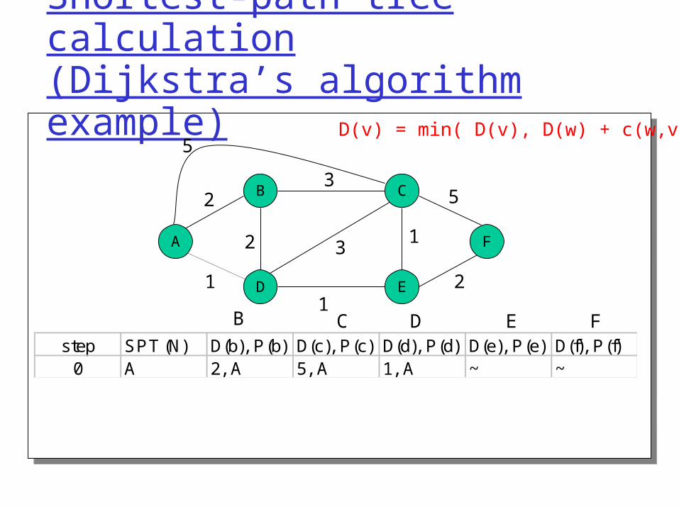
Shortest-path tree calculation(Dijkstra’s algorithm example)

A F

B

D E

C2

2

2

3

1

1

1

3

5

step SPT (N) D(b), P(b) D(c), P(c) D(d), P(d) D(e), P(e) D(f), P(f)0 A 2, A 5, A 1, A ~ ~

5

B C D E F

D(v) = min( D(v), D(w) + c(w,v) )

Dijkstra’s algorithm example

A F

B

D E

C2

2

2

3

1

1

1

3

5

step SPT D(b), P(b) D(c), P(c) D(d), P(d) D(e), P(e) D(f), P(f)0 A 2, A 5, A 1, A ~ ~1 AD 2, A 4, D 2, D ~

5

B C D E F

D(v) = min( D(v), D(w) + c(w,v) )


A F

B

D E

C2

2

2

3

1

1

1

3

5

step SPT D(b), P(b) D(c), P(c) D(d), P(d) D(e), P(e) D(f), P(f)0 A 2, A 5, A 1, A ~ ~1 AD 2, A 4, D 2, D ~2 ADE 2, A 3, E 4, E

5

B C D E F

D(v) = min( D(v), D(w) + c(w,v) )


A F

B

D E

C2

2

2

3

1

1

1

3

5

step SPT D(b), P(b) D(c), P(c) D(d), P(d) D(e), P(e) D(f), P(f)0 A 2, A 5, A 1, A ~ ~1 AD 2, A 4, D 2, D ~2 ADE 2, A 3, E 4, E3 ADEB 3, E 4, E

5

B C D E F

D(v) = min( D(v), D(w) + c(w,v) )


A F

B

D E

C2

2

2

3

1

1

1

3

5

step SPT D(b), P(b) D(c), P(c) D(d), P(d) D(e), P(e) D(f), P(f)0 A 2, A 5, A 1, A ~ ~1 AD 2, A 4, D 2, D ~2 ADE 2, A 3, E 4, E3 ADEB 3, E 4, E4 ADEBC 4, E

5

B C D E F

D(v) = min( D(v), D(w) + c(w,v) )


A F

B

D E

C2

2

2

3

1

1

1

3

5

step SPT D(b), P(b) D(c), P(c) D(d), P(d) D(e), P(e) D(f), P(f)0 A 2, A 5, A 1, A ~ ~1 AD 2, A 4, D 2, D ~2 ADE 2, A 3, E 4, E3 ADEB 3, E 4, E4 ADEBC 4, E5 ADEBCF

5

B C D E F

D(v) = min( D(v), D(w) + c(w,v) )


A

ED

CB

F

Resulting shortest-path tree from A:

BDECF

(A,B)(A,D)(A,D)(A,D)(A,D)

destination linkResulting forwarding table in A:

Dynamic Programming View Dijkstra’s Algorithm: Successive approximation

scheme that solves the dynamic programming equation for the shortest path problem.

If a node is on the minimal path from P to Q, then the part of the path from P to R must be also the optimal path from P to R (Principle of Optimality)

P QR

Link state algorithm characteristics Computation overhead

n nodes each iteration: need to check all

nodes, w, not in N• n*(n+1)/2 comparisons: O(n2)• more efficient implementations

possible: O(n log(n)) Space requirements

Size of LSDB Bandwidth requirements

Reliable broadcast O(N*E) Looping

Consistent LSDBs required for loop-free paths

A

B

C

D

1

3

5 2

1

Packet from CAmay loop around BDCif B knows about failureand C & D do not

X

Link-state algorithm issuesOscillations possible: e.g., link cost = amount of carried traffic Example: path to A flaps as traffic routed

clockwise and counter-clockwise Common problem in load-based link metrics

AD

CB

1 1+e

e0

e1 1

0 0A

DC

B2+e 0

001+e1

AD

CB

0 2+e

1+e10 0

AD

CB

2+e 0

e01+e1

initially … recomputerouting

… recompute … recompute

Distance vector routing algorithms Distributed next hop computation

“Gossip with immediate neighbours until you find the best route”

Best route is achieved when there are no more changes

Unit of information exchange Vector of distances to destinations

Distance Vector Algorithm Bellman-Ford algorithm (1957)DefineDx(y) := cost of least-cost path from x to y

Then

Dx(y) = min {c(x,v) + Dv(y) }

where min is taken over all neighbors v of x

v

Bellman-Ford example

u

yx

wv

z2

21 3

1

12

53

5

Clearly, Dv(z) = 5, Dx(z) = 3, Dw(z) = 3

Du(z) = min { c(u,v) + Dv(z), c(u,x) + Dx(z), c(u,w) + Dw(z) }

= min {2 + 5, 1 + 3, 5 + 3} = 4

Node that achieves minimum is nexthop in shortest path ➜ forwarding table

B-F equation says:

Bellman-Ford Update distance information iteratively

Start with link table (as with Dijkstra), calculate distance table iteratively

Distance table data structure• table of known distances and next hops kept per node• row for each possible destination• column for each directly-attached neighbor to node

A

E D

CB78

12

1

2

DE()ABCD

A1764

B1489

11

D5542

cost to destination via

dest

inat

ion

Distance table at node E

Dj(k,*)

Bellman-Ford algorithm Centralized version

i j

k

j’ k’

c(i,j)

c(i,j’)

Dj’(k,*)

Di(k,*)

For node i

while there is a change in D

for all k not neighbor of i

for each j neighbor of i

Di(k,j) = c(i,j) + Dj(k,*)

if Di(k,j) < Di(k,*) {

Di(k,*) = Di(k,j)

Hi(k) = j

}

DX(Y,Z)

distance from X toY, via Z as next hop

c(X,Z) + min {DZ(Y,w)}w

=

=

DX(Y,*)Minimum known distance from X to Y=

HX(Y) =Next hop node from X to Y

Distance table example for node E

A

E D

CB78

12

1

2DE()

A

B

C

D

A

1

7

6

4

B

14

8

9

11

D

5

5

4

2


dest

inat

ion

DE(C,D) c(E,D) + min {DD(C,w)}w== 2+2 = 4

DE(A,D) c(E,D) + min {DD(A,w)}w== 2+3 = 5

DE(A,B) c(E,B) + min {DB(A,w)}w== 8+6 = 14

loop!

loop! HX(Y) =

Distance table gives forwarding table

D ()

A

B

C

D

A

1

7

6

4

B

14

8

9

11

D

5

5

4

2

E


dest

inat

ion

A

B

C

D

A,1

D,5

D,4

D,4

Outgoing link to use, cost

dest

inat

ion

Distance table Routing table

H (Y)X

Distributed Bellman-Ford Make Bellman algorithm distributed (Ford-Fulkerson

1962) Each node i has distance vector estimates to other nodes Iterate

• Each node sends around and recalculates D[i,*]• When a node x receives new DV estimate from neighbor, it

updates its own DV using B-F equation:

• If estimates change, broadcast entire table to neighbors– continues until no nodes exchange info.– self-terminating: no “signal” to stop

D[i,*] eventually converges to shortest distance

Dx(y) ← minv{c(x,v) + Dv(y)} for each node y ∊ N

Distributed Bellman-Ford overviewAsynchronous: “triggered updates”

no need to exchange info/iterate in lock step!

Iterative: When local link costs change When neighbor sends a

message that its least cost path has changed for a node

Distributed: nodes communicate only with

directly-attached neighbors each node notifies neighbors

only when its least cost path to any destination changes

neighbors then notify their neighbors if necessary

wait for (change in local link cost of msg from neighbor)

recompute distance table

if least cost path to any dest has changed, notify neighbors

Each node:

Distributed Bellman-Ford algorithm

1 Initialization: 2 for all adjacent nodes v: 3 DX(*,v) = infinity /* the * operator means "for all rows" */ 4 DX(v,v) = c(X,v) 5 for all destinations, y 6 send minw (DX(y,w)) to each neighbor /* w over all X's neighbors */

At all nodes, X:

Distributed Bellman-Ford algorithm8 loop 9 wait (until I see a link cost change to neighbor V 10 or until I receive update from neighbor V) 11 12 if (c(X,V) changes by d) 13 /* change cost to all dest's via neighbor v by d */ 14 /* note: d could be positive or negative */ 15 for all destinations y: DX(y,V) = DX(y,V) + d 16 17 else if (update received from V wrt destination Y) 18 /* shortest path from V to some Y has changed */ 19 /* V has sent a new value for its minw (DV(Y,w)) */ 20 /* call this received new value is "newval" */ 21 for the single destination Y: DX(Y,V) = c(X,V) + newval 22 23 if we have a new minw(DX(Y,w)for any destination Y 24 send new value of minw(DX(Y,w)) to all neighbors 25 26 forever

Analyzing Distributed Bellman-Ford Continuously send local distance tables of best

known routes to all neighbors until your table converges Computation diffuses until all nodes converge Will computation converge quickly and

deterministically?• Not all the time, pathologic cases possible (count-

to-infinity)• Several algorithms for minimizing such cases

DBF example

A

B

E

C

D

Info atNode

AB

C

D

A B C

0 7 ~

7 0 1~ 1 0

~ ~ 2

7

1

1

2

28

Distance to Node

D

~

~2

0

E 1 8 ~ 2

1

8~

2

0

E

Initial Distance Vectors

DBF example

Info atNode

AB

C

D

A B C

0 7 ~

7 0 1~ 1 0

~ ~ 2

Distance to Node

D

~

~2

0

E 1 8 ~ 2

1

8~

2

0

E

A

B

E

C

D

7

1

1

2

28

What is the new distance table at E after E receives D’s Routes?

DBF example

Info atNode

AB

C

D

A B C

0 7 ~

7 0 1~ 1 0

~ ~ 2

Distance to Node

D

~

~2

0

E 1 8 4 2

1

8~

2

0

E

A

B

E

C

D

7

1

1

2

28

What is the new distance table at E after E receives D’s Routes?Cost to C is updated from ~ to 4

DBF example

Info atNode

AB

C

D

A B C

0 7 ~

7 0 1~ 1 0

~ ~ 2

Distance to Node

D

~

~2

0

E 1 8 4 2

1

8~

2

0

E

A

B

E

C

D

7

1

1

2

28

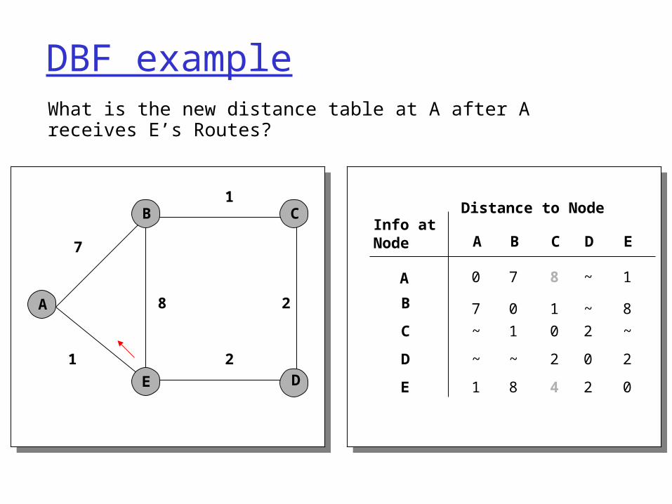
What is the new distance table at A after A receives B’s Routes?

DBF example

Info atNode

AB

C

D

A B C

0 7 8

7 0 1~ 1 0

~ ~ 2

Distance to Node

D

~

~2

0

E 1 8 4 2

1

8~

2

0

E

A

B

E

C

D

7

1

1

2

28

What is the new distance table at A after A receives B’s Routes?Cost to C is updated from ~ to 8, cost to E unchanged

DBF example

Info atNode

AB

C

D

A B C

0 7 8

7 0 1~ 1 0

~ ~ 2

Distance to Node

D

~

~2

0

E 1 8 4 2

1

8~

2

0

E

A

B

E

C

D

7

1

1

2

28

What is the new distance table at A after A receives E’s Routes?

DBF example

Info atNode

AB

C

D

A B C

0 7 5

7 0 1~ 1 0

~ ~ 2

Distance to Node

D

3

~2

0

E 1 8 4 2

1

8~

2

0

E

A

B

E

C

D

7

1

1

2

28

What is the new distance table at A after A receives E’s Routes?Cost to C is updated from 8 to 5, cost to D updated from ~ to 3

DBF example

Info atNode

AB

C

D

A B C

0 6 5

6 0 15 1 0

3 3 2

Distance to Node

D

3

32

0

E 1 5 4 2

1

54

2

0

E

A

B

E

C

D

7

1

1

2

28

And so on, until final distances....

DBF example

dest

AB

C

D

A B D

1 14 5

7 8 56 9 4

4 11 2

Next hop

E’s routing table

A

B

E

C

D

7

1

1

2

28

E’s routing table

DBF (another example)

X Z12

7

Y

DX(Y,Z) c(X,Z) + min {DZ(Y,w)}w=

= 7+1 = 8

DX(Z,Y) c(X,Y) + min {DY(Z,w)}w== 2+1 = 3

DBF (another example)

X Z12

7

Y

DBF (good news example)Link cost changes:• node detects local link cost change • updates distance table (line 15)• if cost change in least cost path, notify

neighbors (lines 23,24)• fast convergence

X Z14

50

Y1

DBF (good news example)

x z14

50

y1

t0) y detects link-cost change, updates its DV, informs neighbors.

t1) z receives the update from y and updates its table. It computes a new least cost to x and sends its neighbors its DV.

t2) y receives z’s update and updates its distance table. y’s least costs do not change and hence y does not send any message to z.

algorithmterminates“good

news travelsfast”

DBF (count-to-infinity example)Link cost changes:• good news travels fast • bad news travels slow - “count to infinity” problem!• alternate route implicitly used link that changed

X Z14

50

Y60

algorithmcontinues

on!

How are loops caused? Observation 1:

Y’s metric to X increases Observation 2:

Z picks Y as next hop to X But, the implicit path from Z to X includes itself!

DBF: (count-to-infinity example)

A

25

1

1

B

C

BC 2

1

dest cost

AC 1

1

dest cost

AB 1

2

dest cost

X


A

25 1

B

C

BC 2

1

dest cost

AC 1

~

dest cost

AB 1

2

dest cost

C Sends Routes to B


A

25 1

B

C

BC 2

1

dest cost

AC 1

3

dest cost

AB 1

2

dest cost

B Updates Distance to A


A

25 1

B

C

BC 2

1

dest cost

AC 1

3

dest cost

AB 1

4

dest cost

B Sends Routes to C


A

25 1

B

C

BC 2

1

dest cost

AC 1

5

dest cost

AB 1

4

dest cost

C Sends Routes to B

Solutions to looping Split horizon

Do not advertise route to X to an adjacent neighbor if your route to X goes through that neighbor

If C routes through B to get to A, C does not advertise (C=>A) route to B.

Poisoned reverse Advertise an infinite distance route to X to an

adjacent neighbor if your route to X goes through that neighbor

If C routes through B to get to A, C advertises to B that its distance to A is infinity

Split-horizon with poisoned reverseIf Z routes through Y to get to X :• Z tells Y its (Z’s) distance to X is infinite (so

Y won’t route to X via Z)• will this completely solve count to infinity

problem? X Z

14

50

Y60

algorithmterminates

new route to X not involving Y

can now select and advertise route to X via Z

route to X through Y goes thru Zpoison it!

Comparing link-state vs. distance vector Communication costs Processing costs Optimality Convergence issues

Convergence time Loop freedom Oscillation damping

Message complexity, network bandwidth LS: with n nodes, E links, O(nE) msgs sent

Send info about your neighbors to everyone Small messages broadcast globally

DV: exchange between neighbors onlySend everything you know to your

neighborsLarge messages, but transfers only to

neighbors

Link State vs. Distance Vector

Link State vs. Distance VectorSpeed of Convergence LS: O(n2) algorithm requires O(nE) msgs

Faster – can forward LSPs before processing

Single SPT calculation DV: convergence time varies

Fast with triggered updatescount-to-infinity problemmay be routing loops

Link State vs. Distance VectorSpace requirements:LS: maintains entire topologyDV: maintains only neighbor state

path vector maintains routes proportional to network diameter

Link State vs. Distance VectorRobustness:LS

Can be made robust since sources are aware of alternate paths within topology

DVCan advertise incorrect paths to all

destinationsIncorrect calculation can spread to entire

network

Hierarchical Routing

scale: with 200 million destinations:

can’t store all dest’s in routing tables!

routing table exchange would swamp links!

Flat routing does not scale

administrative autonomy

internet = network of networks

each network admin may want to control routing in its own network

Our routing study thus far - idealization all routers identical network “flat”… not true in practice

Hierarchical Routing Divide network into areas

Within area, each node has routes to every other node

Outside area• Each node has routes for other top-level areas only (not

nodes within those areas)• Inter-area packets are routed to nearest appropriate

border router

Internet Routing Hierarchy

Internet areas called “autonomous systems” (AS) administrative

autonomy routers in same AS

run same routing protocol “intra-AS” routing

protocol (IGP) Each AS can run its

own intra-AS routing protocol

Border routers Special routers in AS

that directly link to another AS

Responsible for routing to destinations outside AS

• run intra-AS routing protocol with all other routers in AS

• run inter-AS routing protocol or exterior gateway protocol (EGP) with other gateway routers in other AS’s

Internet Routing HierarchyBorder router A.c

Routing protocols• Inter-AS

externally• Intra-AS internally

Forwarding table configured by both

network layerlink layer

physical layer

a

b

ba

aC

A

Bd

A.aA.c

C.bB.a

cb

c

ForwardingTable

Why different Intra- and Inter-AS routing ? Policy: Intra-AS: single administrative policy

No policy decisions needed, performance dominates

Focus on performance Inter-AS: ISP wants control over how its

traffic routed, who routes through its net. Policy and monetary factors dominate over

performance

3b

1d

3a1c

2aAS3

AS1AS21a

2c2b

1b

3c

Inter-AS tasks Suppose router in AS1

receives datagram for destination outside of AS1 router should

forward packet to gateway router, but which one?

AS1 must:1. learn which dests

reachable through AS2, which through AS3

2. propagate this reachability info to all routers in AS1

Job of inter-AS routing!

Example: Setting forwarding table in router 1d

suppose AS1 learns (via inter-AS protocol) that subnet x reachable via AS3 (gateway 1c) but not via AS2.

inter-AS protocol propagates reachability info to all internal routers.

router 1d determines from intra-AS routing info that its interface I is on the least cost path to 1c. installs forwarding table entry (x,I)

3b

1d

3a1c

2aAS3

AS1AS21a

2c2b

1b

3cx…

Example: Choosing among multiple ASes now suppose AS1 learns from inter-AS protocol

that subnet x is reachable from AS3 and from AS2.

to configure forwarding table, router 1d must determine towards which gateway it should forward packets for dest x. this is also the job of inter-AS routing

protocol!

3b

1d

3a1c

2aAS3

AS1AS21a

2c2b

1b

3cx… …

Learn from inter-AS protocol that subnet x is reachable via multiple gateways

Use routing infofrom intra-AS

protocol to determine

costs of least-cost paths to each

of the gateways

Choose the gateway

that has the smallest least cost

Determine fromforwarding table the interface I that leads

to least-cost gateway. Enter (x,I) in

forwarding table

Example: Choosing among multiple ASes Cost-based selection

Internet Routing Protocols Intra-AS routing protocols, also known as

Interior Gateway Protocols (IGP) RIP: Routing Information Protocol

• Distance-vector

OSPF: Open Shortest Path First• Link-state

IGRP: Interior Gateway Routing Protocol (Cisco proprietary)

• Distance-vector Inter-AS routing: BGP (Border Gateway Protocol)

R1

R2

R3 R4

sourceduplication

R1

R2

R3 R4

in-networkduplication

duplicatecreation/transmissionduplicate

duplicate

Broadcast Routing deliver packets from source to all other nodes source duplication is inefficient:

source duplication: how does source determine recipient addresses?

In-network duplication flooding: when node receives brdcst pckt,

sends copy to all neighbors Problems: cycles & broadcast storm

controlled flooding: node only brdcsts pkt if it hasn’t brdcst same packet before Node keeps track of pckt ids already brdcsted Or reverse path forwarding (RPF): only forward

pckt if it arrived on shortest path between node and source

spanning tree No redundant packets received by any node

A

B

G

DE

c

F

A

B

G

DE

c

F

(a) Broadcast initiated at A (b) Broadcast initiated at D

Spanning Tree First construct a spanning tree Nodes forward copies only along

spanning tree

A

B

G

DE

c

F1

2

3

4

5

(a) Stepwise construction of spanning tree

A

B

G

DE

c

F

(b) Constructed spanning tree

Spanning Tree: Creation Center node Each node sends unicast join message to

center node Message forwarded until it arrives at a node already

belonging to spanning tree

Multicast Routing: Problem Statement Goal: find a tree (or trees) connecting

routers having local mcast group members tree: not all paths between routers used source-based: different tree from each sender to rcvrs shared-tree: same tree used by all group members

Shared tree Source-based trees

Approaches for building mcast treesApproaches: source-based tree: one tree per source

minimum spanning tree (Prim and Kruskal algorithms, not discussed here)

shortest path trees reverse path forwarding

group-shared tree: group uses one tree minimal spanning (Steiner) center-based trees

Shortest Path Tree mcast forwarding tree: tree of shortest

path routes from source to all receivers Dijkstra’s algorithm

R1

R2

R3

R4

R5

R6 R7

21

6

3 45

i

router with attachedgroup member

router with no attachedgroup memberlink used for forwarding,i indicates order linkadded by algorithm

LEGENDS: source

Reverse Path Forwarding

if (mcast datagram received on incoming link on shortest path back to center)

then flood datagram onto all outgoing links else ignore datagram

rely on router’s knowledge of unicast shortest path from it to sender

each router has simple forwarding behavior:

Reverse Path Forwarding: example

• result is a source-specific reverse SPT– may be a bad choice with asymmetric links

R1

R2

R3

R4

R5

R6 R7

router with attachedgroup member

router with no attachedgroup memberdatagram will be forwarded

LEGENDS: source

datagram will not be forwarded

Reverse Path Forwarding: pruning forwarding tree contains subtrees with no mcast

group members no need to forward datagrams down subtree “prune” msgs sent upstream by router with

no downstream group members

R1

R2

R3

R4

R5

R6 R7

router with attachedgroup memberrouter with no attachedgroup memberprune message

LEGENDS: source

links with multicastforwarding

P

P

P

Shared-Tree: Steiner Tree

Steiner Tree: minimum cost tree connecting all routers with attached group members

problem is NP-complete excellent heuristics exists not used in practice:

computational complexity information about entire network needed monolithic: rerun whenever a router needs

to join/leave

Center-based trees single delivery tree shared by all one router identified as “center” of tree to join:

edge router sends unicast join-msg addressed to center router

join-msg “processed” by intermediate routers and forwarded towards center

join-msg either hits existing tree branch for this center, or arrives at center

path taken by join-msg becomes new branch of tree for this router

Center-based trees: an exampleSuppose R6 chosen as center:

R1

R2

R3

R4

R5

R6 R7

router with attachedgroup memberrouter with no attachedgroup memberpath order in which join messages generated

LEGEND

21

3

1

TunnelingQ: How to connect “islands” of multicast

routers in a “sea” of unicast routers?

mcast datagram encapsulated inside “normal” (non-multicast-addressed) datagram normal IP datagram sent thru “tunnel” via regular IP unicast to receiving mcast router receiving mcast router unencapsulates to get mcast datagram

physical topology logical topology

Lecture 13, 14: Routing Algorithms ELEN E6761: Communication Networks Instructor: Javad Ghaderi...

Documents

Transcript of Lecture 13, 14: Routing Algorithms ELEN E6761: Communication Networks Instructor: Javad Ghaderi...