
Lecture 12: Fast Reinforcement Learning Part II...
70
Lecture 12: Fast Reinforcement Learning Part II 2 Emma Brunskill CS234 Reinforcement Learning. Winter 2018 2 With many slides from or derived from David Silver, Worked Examples New Emma Brunskill (CS234 Reinforcement Learning. ) Lecture 12: Fast Reinforcement Learning Part II Winter 2018 1 / 70
Transcript of Lecture 12: Fast Reinforcement Learning Part II...

Lecture 12: Fast Reinforcement Learning Part II 2
Emma Brunskill
CS234 Reinforcement Learning.
Winter 2018
2With many slides from or derived from David Silver, Worked Examples NewEmma Brunskill (CS234 Reinforcement Learning. )Lecture 12: Fast Reinforcement Learning Part II 3 Winter 2018 1 / 70

Class Structure
Last time: Fast Learning, Exploration/Exploitation Part 1
This Time: Fast Learning Part II
Next time: Batch RL
Emma Brunskill (CS234 Reinforcement Learning. )Lecture 12: Fast Reinforcement Learning Part II 4 Winter 2018 2 / 70

Table of Contents
1 Metrics for evaluating RL algorithms
2 Principles for RL Exploration
3 Probability Matching
4 Information State Search
5 MDPs
6 Principles for RL Exploration
7 Metrics for evaluating RL algorithms
Emma Brunskill (CS234 Reinforcement Learning. )Lecture 12: Fast Reinforcement Learning Part II 5 Winter 2018 3 / 70

Performance Criteria of RL Algorithms
Empirical performance
Convergence (to something ...)
Asymptotic convergence to optimal policy
Finite sample guarantees: probably approximately correct
Regret (with respect to optimal decisions)
Optimal decisions given information have available
PAC uniform
Emma Brunskill (CS234 Reinforcement Learning. )Lecture 12: Fast Reinforcement Learning Part II 6 Winter 2018 4 / 70

Table of Contents
1 Metrics for evaluating RL algorithms
2 Principles for RL Exploration
3 Probability Matching
4 Information State Search
5 MDPs
6 Principles for RL Exploration
7 Metrics for evaluating RL algorithms
Emma Brunskill (CS234 Reinforcement Learning. )Lecture 12: Fast Reinforcement Learning Part II 7 Winter 2018 5 / 70

Principles
Naive Exploration (last time)
Optimistic Initialization (last time)
Optimism in the Face of Uncertainty (last time + this time)
Probability Matching (last time + this time)
Information State Search (this time)
Emma Brunskill (CS234 Reinforcement Learning. )Lecture 12: Fast Reinforcement Learning Part II 8 Winter 2018 6 / 70

Multiarmed Bandits
Multi-armed bandit is a tuple of (A,R)
A : known set of m actions
Ra(r) = P[r | a] is an unknown probability distribution over rewards
At each step t the agent selects an action at ∈ AThe environment generates a reward rt ∼ Rat
Goal: Maximize cumulative reward∑t
τ=1 rτ
Emma Brunskill (CS234 Reinforcement Learning. )Lecture 12: Fast Reinforcement Learning Part II 9 Winter 2018 7 / 70
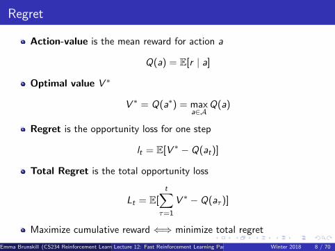
Regret
Action-value is the mean reward for action a
Q(a) = E[r | a]
Optimal value V ∗
V ∗ = Q(a∗) = maxa∈A
Q(a)
Regret is the opportunity loss for one step
lt = E[V ∗ − Q(at)]
Total Regret is the total opportunity loss
Lt = E[t∑
τ=1
V ∗ − Q(aτ )]
Maximize cumulative reward ⇐⇒ minimize total regret
Emma Brunskill (CS234 Reinforcement Learning. )Lecture 12: Fast Reinforcement Learning Part II 10 Winter 2018 8 / 70
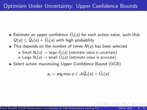
Optimism Under Uncertainty: Upper Confidence Bounds
Estimate an upper confidence Ut(a) for each action value, such thatQ(a) ≤ Qt(a) + Ut(a) with high probability
This depends on the number of times N(a) has been selected
Small Nt(a)→ large Ut(a) (estimate value is uncertain)Large Nt(a)→ small Ut(a) (estimate value is accurate)
Select action maximizing Upper Confidence Bound (UCB)
at = arg max a ∈ AQt(a) + Ut(a)
Emma Brunskill (CS234 Reinforcement Learning. )Lecture 12: Fast Reinforcement Learning Part II 11 Winter 2018 9 / 70
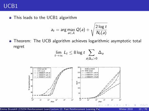
UCB1
This leads to the UCB1 algorithm
at = arg maxa∈A
Q(a) +
√2 log t
Nt(a)
Theorem: The UCB algorithm achieves logarithmic asymptotic totalregret
limt→∞
Lt ≤ 8 log t∑
a|∆a>0
∆a
Emma Brunskill (CS234 Reinforcement Learning. )Lecture 12: Fast Reinforcement Learning Part II 12 Winter 2018 10 / 70
Toy Example: Ways to Treat Broken Toes13
Consider deciding how to best treat patients with broken toes
Imagine have 3 possible options: (1) surgery (2) buddy taping thebroken toe with another toe, (3) do nothing
Outcome measure is binary variable: whether the toe has healed (+1)or not healed (0) after 6 weeks, as assessed by x-ray
13Note:This is a made up example. This is not the actual expected efficacies of thevarious treatment options for a broken toe
Emma Brunskill (CS234 Reinforcement Learning. )Lecture 12: Fast Reinforcement Learning Part II 14 Winter 2018 11 / 70

Toy Example: Ways to Treat Broken Toes15
Consider deciding how to best treat patients with broken toes
Imagine have 3 common options: (1) surgery (2) surgical boot (3)buddy taping the broken toe with another toe
Outcome measure is binary variable: whether the toe has healed (+1)or not (0) after 6 weeks, as assessed by x-ray
Model as a multi-armed bandit with 3 arms, where each arm is aBernoulli variable with an unknown parameter θi
Check your understanding: what does a pull of an arm / taking anaction correspond to? Why is it reasonable to model this as amulti-armed bandit instead of a Markov decision process?
15Note:This is a made up example. This is not the actual expected efficacies of thevarious treatment options for a broken toe
Emma Brunskill (CS234 Reinforcement Learning. )Lecture 12: Fast Reinforcement Learning Part II 16 Winter 2018 12 / 70

Toy Example: Ways to Treat Broken Toes17
Imagine true (unknown) parameters for each arm (action) are
surgery: Q(a1) = θ1 = .95buddy taping: Q(a2) = θ2 = .9doing nothing: Q(a3) = θ3 = .1
17Note:This is a made up example. This is not the actual expected efficacies of thevarious treatment options for a broken toe
Emma Brunskill (CS234 Reinforcement Learning. )Lecture 12: Fast Reinforcement Learning Part II 18 Winter 2018 13 / 70

Toy Example: Ways to Treat Broken Toes, ThompsonSampling19
True (unknown) parameters for each arm (action) are
surgery: Q(a1) = θ1 = .95buddy taping: Q(a2) = θ2 = .9doing nothing: Q(a3) = θ3 = .1
Optimism under uncertainty, UCB1 (Auer, Cesa-Bianchi, Fischer2002)
1 Sample each arm once
19Note:This is a made up example. This is not the actual expected efficacies of thevarious treatment options for a broken toe
Emma Brunskill (CS234 Reinforcement Learning. )Lecture 12: Fast Reinforcement Learning Part II 20 Winter 2018 14 / 70
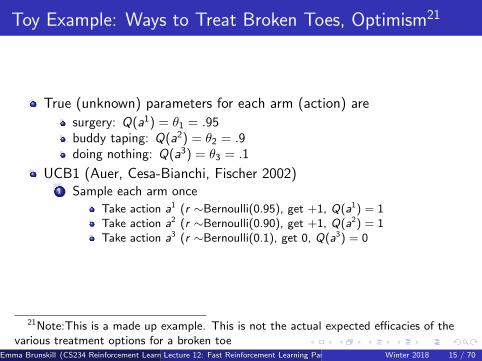
Toy Example: Ways to Treat Broken Toes, Optimism21
True (unknown) parameters for each arm (action) are
surgery: Q(a1) = θ1 = .95buddy taping: Q(a2) = θ2 = .9doing nothing: Q(a3) = θ3 = .1
UCB1 (Auer, Cesa-Bianchi, Fischer 2002)1 Sample each arm once
Take action a1 (r ∼Bernoulli(0.95), get +1, Q(a1) = 1Take action a2 (r ∼Bernoulli(0.90), get +1, Q(a2) = 1Take action a3 (r ∼Bernoulli(0.1), get 0, Q(a3) = 0
21Note:This is a made up example. This is not the actual expected efficacies of thevarious treatment options for a broken toe
Emma Brunskill (CS234 Reinforcement Learning. )Lecture 12: Fast Reinforcement Learning Part II 22 Winter 2018 15 / 70

Toy Example: Ways to Treat Broken Toes, Optimism23
True (unknown) parameters for each arm (action) are
surgery: Q(a1) = θ1 = .95buddy taping: Q(a2) = θ2 = .9doing nothing: Q(a3) = θ3 = .1
UCB1 (Auer, Cesa-Bianchi, Fischer 2002)1 Sample each arm once
Take action a1 (r ∼Bernoulli(0.95), get +1, Q(a1) = 1Take action a2 (r ∼Bernoulli(0.90), get +1, Q(a2) = 1Take action a3 (r ∼Bernoulli(0.1), get 0, Q(a3) = 0
2 Set t = 3, Compute upper confidence bound on each action
ucb(a) = Q(a) +
√2lnt
Nt(a)
23Note:This is a made up example. This is not the actual expected efficacies of thevarious treatment options for a broken toe
Emma Brunskill (CS234 Reinforcement Learning. )Lecture 12: Fast Reinforcement Learning Part II 24 Winter 2018 16 / 70

Toy Example: Ways to Treat Broken Toes, Optimism25
True (unknown) parameters for each arm (action) aresurgery: Q(a1) = θ1 = .95buddy taping: Q(a2) = θ2 = .9doing nothing: Q(a3) = θ3 = .1
UCB1 (Auer, Cesa-Bianchi, Fischer 2002)1 Sample each arm once
Take action a1 (r ∼Bernoulli(0.95), get +1, Q(a1) = 1Take action a2 (r ∼Bernoulli(0.90), get +1, Q(a2) = 1Take action a3 (r ∼Bernoulli(0.1), get 0, Q(a3) = 0
2 Set t = 3, Compute upper confidence bound on each action
ucb(a) = Q(a) +
√2lnt
Nt(a)
3 t = 3, Select action at = arg maxa ucb(a),4 Observe reward 15 Compute upper confidence bound on each action
25Note:This is a made up example. This is not the actual expected efficacies of thevarious treatment options for a broken toe
Emma Brunskill (CS234 Reinforcement Learning. )Lecture 12: Fast Reinforcement Learning Part II 26 Winter 2018 17 / 70

Toy Example: Ways to Treat Broken Toes, Optimism27
True (unknown) parameters for each arm (action) aresurgery: Q(a1) = θ1 = .95buddy taping: Q(a2) = θ2 = .9doing nothing: Q(a3) = θ3 = .1
UCB1 (Auer, Cesa-Bianchi, Fischer 2002)1 Sample each arm once
Take action a1 (r ∼Bernoulli(0.95), get +1, Q(a1) = 1Take action a2 (r ∼Bernoulli(0.90), get +1, Q(a2) = 1Take action a3 (r ∼Bernoulli(0.1), get 0, Q(a3) = 0
2 Set t = 3, Compute upper confidence bound on each action
ucb(a) = Q(a) +
√2lnt
Nt(a)
3 t = t + 1, Select action at = arg maxa ucb(a),4 Observe reward 15 Compute upper confidence bound on each action
27Note:This is a made up example. This is not the actual expected efficacies of thevarious treatment options for a broken toe
Emma Brunskill (CS234 Reinforcement Learning. )Lecture 12: Fast Reinforcement Learning Part II 28 Winter 2018 18 / 70
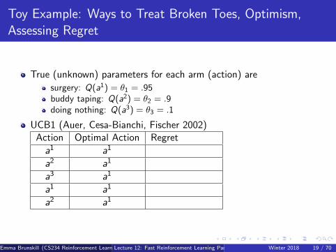
Toy Example: Ways to Treat Broken Toes, Optimism,Assessing Regret
True (unknown) parameters for each arm (action) are
surgery: Q(a1) = θ1 = .95buddy taping: Q(a2) = θ2 = .9doing nothing: Q(a3) = θ3 = .1
UCB1 (Auer, Cesa-Bianchi, Fischer 2002)Action Optimal Action Regret
a1 a1
a2 a1
a3 a1
a1 a1
a2 a1
Emma Brunskill (CS234 Reinforcement Learning. )Lecture 12: Fast Reinforcement Learning Part II 29 Winter 2018 19 / 70
Check Your Understanding
An alternative would be to always select the arm with the highestlower bound
Why can this yield linear regret?
Consider a two arm case for simplicity
Emma Brunskill (CS234 Reinforcement Learning. )Lecture 12: Fast Reinforcement Learning Part II 30 Winter 2018 20 / 70

Table of Contents
1 Metrics for evaluating RL algorithms
2 Principles for RL Exploration
3 Probability Matching
4 Information State Search
5 MDPs
6 Principles for RL Exploration
7 Metrics for evaluating RL algorithms
Emma Brunskill (CS234 Reinforcement Learning. )Lecture 12: Fast Reinforcement Learning Part II 31 Winter 2018 21 / 70

Probability Matching
Assume have a parametric distribution over rewards for each arm
Probability matching selects action a according to probability that ais the optimal action
π(a | ht) = P[Q(a) > Q(a′), ∀a′ 6= a | ht ]
Probability matching is optimistic in the face of uncertainty
Uncertain actions have higher probability of being max
Can be difficult to compute analytically from posterior
Emma Brunskill (CS234 Reinforcement Learning. )Lecture 12: Fast Reinforcement Learning Part II 32 Winter 2018 22 / 70

Thompson sampling implements probability matching
Thompson sampling:
π(a | ht) = P[Q(a) > Q(a′), ∀a′ 6= a | ht ]
= ER|ht
[1(a = arg max
a∈AQ(a))
]
Emma Brunskill (CS234 Reinforcement Learning. )Lecture 12: Fast Reinforcement Learning Part II 33 Winter 2018 23 / 70

Thompson sampling implements probability matching
Thompson sampling:
π(a | ht) = P[Q(a) > Q(a′), ∀a′ 6= a | ht ]
= ER|ht
[1(a = arg max
a∈AQ(a))
]Use Bayes law to compute posterior distribution p[R | ht ]Sample a reward distribution R from posterior
Compute action-value function Q(a) = E[Ra]
Select action maximizing value on sample, at = arg maxa∈AQ(a)
Emma Brunskill (CS234 Reinforcement Learning. )Lecture 12: Fast Reinforcement Learning Part II 34 Winter 2018 24 / 70

Thompson sampling implements probability matching
Thompson sampling achieves Lai and Robbins lower bound
Last checked: bounds for optimism are tighter than for Thomsponsampling
But empirically Thompson sampling can be extremely effective
Emma Brunskill (CS234 Reinforcement Learning. )Lecture 12: Fast Reinforcement Learning Part II 35 Winter 2018 25 / 70

Thompson Sampling for News Article Recommendation(Chapelle and Li, 2010)
Contextual bandit: input context which impacts reward of each arm,context sampled iid each step
Arms = articles
Reward = click (+1) on article (Q(a)=click through rate)
Emma Brunskill (CS234 Reinforcement Learning. )Lecture 12: Fast Reinforcement Learning Part II 36 Winter 2018 26 / 70
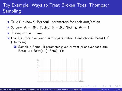
Toy Example: Ways to Treat Broken Toes, ThompsonSampling
True (unknown) Bernoulli parameters for each arm/action
Surgery: θ1 = .95 / Taping: θ2 = .9 / Nothing: θ3 = .1
Thompson sampling:
Place a prior over each arm’s parameter. Here choose Beta(1,1)(Uniform)
1 Sample a Bernoulli parameter given current prior over each armBeta(1,1), Beta(1,1), Beta(1,1):
Emma Brunskill (CS234 Reinforcement Learning. )Lecture 12: Fast Reinforcement Learning Part II 37 Winter 2018 27 / 70
Toy Example: Ways to Treat Broken Toes, ThompsonSampling38
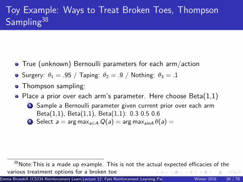
True (unknown) Bernoulli parameters for each arm/action
Surgery: θ1 = .95 / Taping: θ2 = .9 / Nothing: θ3 = .1
Thompson sampling:
Place a prior over each arm’s parameter. Here choose Beta(1,1)1 Sample a Bernoulli parameter given current prior over each arm
Beta(1,1), Beta(1,1), Beta(1,1): 0.3 0.5 0.62 Select a = arg maxa∈A Q(a) = arg maxainA θ(a) =
38Note:This is a made up example. This is not the actual expected efficacies of thevarious treatment options for a broken toe
Emma Brunskill (CS234 Reinforcement Learning. )Lecture 12: Fast Reinforcement Learning Part II 39 Winter 2018 28 / 70
Toy Example: Ways to Treat Broken Toes, ThompsonSampling
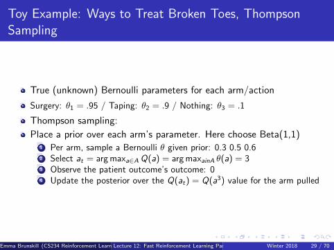
True (unknown) Bernoulli parameters for each arm/action
Surgery: θ1 = .95 / Taping: θ2 = .9 / Nothing: θ3 = .1
Thompson sampling:
Place a prior over each arm’s parameter. Here choose Beta(1,1)1 Per arm, sample a Bernoulli θ given prior: 0.3 0.5 0.62 Select at = arg maxa∈A Q(a) = arg maxainA θ(a) = 33 Observe the patient outcome’s outcome: 04 Update the posterior over the Q(at) = Q(a3) value for the arm pulled
Emma Brunskill (CS234 Reinforcement Learning. )Lecture 12: Fast Reinforcement Learning Part II 40 Winter 2018 29 / 70

Toy Example: Ways to Treat Broken Toes, ThompsonSampling
True (unknown) Bernoulli parameters for each arm/action
Surgery: θ1 = .95 / Taping: θ2 = .9 / Nothing: θ3 = .1
Thompson sampling:
Place a prior over each arm’s parameter. Here choose Beta(1,1)1 Sample a Bernoulli parameter given current prior over each arm
Beta(1,1), Beta(1,1), Beta(1,1): 0.3 0.5 0.62 Select at = arg maxa∈A Q(a) = arg maxainA θ(a) = 33 Observe the patient outcome’s outcome: 04 Update the posterior over the Q(at) = Q(a1) value for the arm pulled
Beta(c1, c2) is the conjugate distribution for BernoulliIf observe 1, c1 + 1 else if observe 0 c2 + 1
5 New posterior over Q value for arm pulled is:6 New posterior p(Q(a3)) = p(θ(a3) = Beta(1, 2)
Emma Brunskill (CS234 Reinforcement Learning. )Lecture 12: Fast Reinforcement Learning Part II 41 Winter 2018 30 / 70

Toy Example: Ways to Treat Broken Toes, ThompsonSampling
True (unknown) Bernoulli parameters for each arm/action
Surgery: θ1 = .95 / Taping: θ2 = .9 / Nothing: θ3 = .1
Thompson sampling:
Place a prior over each arm’s parameter. Here choose Beta(1,1)1 Sample a Bernoulli parameter given current prior over each arm
Beta(1,1), Beta(1,1), Beta(1,1): 0.3 0.5 0.62 Select at = arg maxa∈A Q(a) = arg maxainA θ(a) = 13 Observe the patient outcome’s outcome: 04 New posterior p(Q(a1)) = p(θ(a1) = Beta(1, 2)
Emma Brunskill (CS234 Reinforcement Learning. )Lecture 12: Fast Reinforcement Learning Part II 42 Winter 2018 31 / 70
Toy Example: Ways to Treat Broken Toes, ThompsonSampling
True (unknown) Bernoulli parameters for each arm/action
Surgery: θ1 = .95 / Taping: θ2 = .9 / Nothing: θ3 = .1
Thompson sampling:
Place a prior over each arm’s parameter. Here choose Beta(1,1)1 Sample a Bernoulli parameter given current prior over each arm
Beta(1,1), Beta(1,1), Beta(1,2): 0.7, 0.5, 0.3
Emma Brunskill (CS234 Reinforcement Learning. )Lecture 12: Fast Reinforcement Learning Part II 43 Winter 2018 32 / 70
Toy Example: Ways to Treat Broken Toes, ThompsonSampling
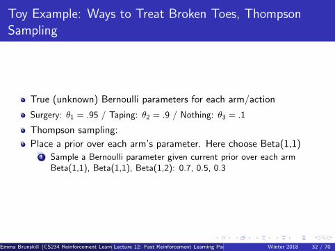
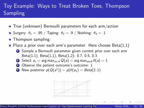
True (unknown) Bernoulli parameters for each arm/action
Surgery: θ1 = .95 / Taping: θ2 = .9 / Nothing: θ3 = .1
Thompson sampling:
Place a prior over each arm’s parameter. Here choose Beta(1,1)1 Sample a Bernoulli parameter given current prior over each arm
Beta(1,1), Beta(1,1), Beta(1,2): 0.7, 0.5, 0.32 Select at = arg maxa∈A Q(a) = arg maxainA θ(a) = 13 Observe the patient outcome’s outcome: 14 New posterior p(Q(a1)) = p(θ(a1) = Beta(2, 1)
Emma Brunskill (CS234 Reinforcement Learning. )Lecture 12: Fast Reinforcement Learning Part II 44 Winter 2018 33 / 70

Toy Example: Ways to Treat Broken Toes, ThompsonSampling
True (unknown) Bernoulli parameters for each arm/action
Surgery: θ1 = .95 / Taping: θ2 = .9 / Nothing: θ3 = .1
Thompson sampling:Place a prior over each arm’s parameter. Here choose Beta(1,1)
1 Sample a Bernoulli parameter given current prior over each armBeta(2,1), Beta(1,1), Beta(1,2): 0.71, 0.65, 0.1
2 Select at = arg maxa∈A Q(a) = arg maxainA θ(a) = 13 Observe the patient outcome’s outcome: 14 New posterior p(Q(a1)) = p(θ(a1) = Beta(3, 1)
Emma Brunskill (CS234 Reinforcement Learning. )Lecture 12: Fast Reinforcement Learning Part II 45 Winter 2018 34 / 70

Toy Example: Ways to Treat Broken Toes, ThompsonSampling
True (unknown) Bernoulli parameters for each arm/actionSurgery: θ1 = .95 / Taping: θ2 = .9 / Nothing: θ3 = .1
Thompson sampling:Place a prior over each arm’s parameter. Here choose Beta(1,1)
1 Sample a Bernoulli parameter given current prior over each armBeta(2,1), Beta(1,1), Beta(1,2): 0.75, 0.45, 0.4
2 Select at = arg maxa∈A Q(a) = arg maxainA θ(a) = 13 Observe the patient outcome’s outcome: 14 New posterior p(Q(a1)) = p(θ(a1) = Beta(4, 1)
Emma Brunskill (CS234 Reinforcement Learning. )Lecture 12: Fast Reinforcement Learning Part II 46 Winter 2018 35 / 70

Toy Example: Ways to Treat Broken Toes, ThompsonSampling vs Optimism
Surgery: θ1 = .95 / Taping: θ2 = .9 / Nothing: θ3 = .1
How does the sequence of arm pulls compare in this example so far?Optimism TS Optimal Regret Optimism Regret TS
a1 a3
a2 a1
a3 a1
a1 a1
a2 a1
Emma Brunskill (CS234 Reinforcement Learning. )Lecture 12: Fast Reinforcement Learning Part II 47 Winter 2018 36 / 70

Toy Example: Ways to Treat Broken Toes, ThompsonSampling vs Optimism
Surgery: θ1 = .95 / Taping: θ2 = .9 / Nothing: θ3 = .1
Incurred regret?Optimism TS Optimal Regret Optimism Regret TS
a1 a3 a1 0 0
a2 a1 a1 0.05
a3 a1 a1 0.85
a1 a1 a1 0
a2 a1 a1 0.05
Emma Brunskill (CS234 Reinforcement Learning. )Lecture 12: Fast Reinforcement Learning Part II 48 Winter 2018 37 / 70

Alternate Metric: Probably Approximately Correct
Theoretical regret bounds specify how regret grows with T
Could be making lots of little mistakes or infrequent large ones
May care about bounding the number of non-small errors
More formally, probably approximately correct (PAC) results statethat the algorithm will choose an action a whose value is ε-optimal(Q(a) ≥ Q(a∗)− ε) with probability at least 1− δ on all but apolynomial number of steps
Polynomial in the problem parameters (# actions, ε, δ, etc)
Exist PAC algorithms based on optimism or Thompson sampling
Emma Brunskill (CS234 Reinforcement Learning. )Lecture 12: Fast Reinforcement Learning Part II 49 Winter 2018 38 / 70

Toy Example: Probably Approximately Correct and Regret
Surgery: θ1 = .95 / Taping: θ2 = .9 / Nothing: θ3 = .1
Let ε = 0.05.
O = Optimism, TS = Thompson Sampling: W/in ε =I (Q(at) ≥ Q(a∗)− ε)
O TS Optimal O Regret O W/in ε TS Regret TS W/in εa1 a3 a1 0 0.85a2 a1 a1 0.05 0a3 a1 a1 0.85 0a1 a1 a1 0 0a2 a1 a1 0.05 0
Emma Brunskill (CS234 Reinforcement Learning. )Lecture 12: Fast Reinforcement Learning Part II 50 Winter 2018 39 / 70

Toy Example: Probably Approximately Correct and Regret
Surgery: θ1 = .95 / Taping: θ2 = .9 / Nothing: θ3 = .1
Let ε = 0.05.
O = Optimism, TS = Thompson Sampling: W/in ε =I (Q(at) ≥ Q(a∗)− ε)
O TS Optimal O Regret O W/in ε TS Regret TS W/in εa1 a3 a1 0 Y 0.85 Na2 a1 a1 0.05 Y 0 Ya3 a1 a1 0.85 N 0 Ya1 a1 a1 0 Y 0 Ya2 a1 a1 0.05 Y 0 Y
Emma Brunskill (CS234 Reinforcement Learning. )Lecture 12: Fast Reinforcement Learning Part II 51 Winter 2018 40 / 70

Table of Contents
1 Metrics for evaluating RL algorithms
2 Principles for RL Exploration
3 Probability Matching
4 Information State Search
5 MDPs
6 Principles for RL Exploration
7 Metrics for evaluating RL algorithms
Emma Brunskill (CS234 Reinforcement Learning. )Lecture 12: Fast Reinforcement Learning Part II 52 Winter 2018 41 / 70
Relevant Background: Value of Information
Exploration is useful because it gains information
Can we quantify the value of information (VOI)?
How much reward a decision-maker would be prepared to pay in orderto have that information, prior to making a decisionLong-term reward after getting information - immediate reward
Emma Brunskill (CS234 Reinforcement Learning. )Lecture 12: Fast Reinforcement Learning Part II 53 Winter 2018 42 / 70

Relevant Background: Value of Information Example
Consider bandit where only get to make a single decision
Oil company considering buying rights to drill in 1 of 5 locations
1 of locations contains $10 million worth of oil, others 0
Cost of buying rights to drill is $2 million
Seismologist says for a fee will survey one of 5 locations and reportback definitively whether that location does or does not contain oil
What should one consider paying seismologist?
Emma Brunskill (CS234 Reinforcement Learning. )Lecture 12: Fast Reinforcement Learning Part II 54 Winter 2018 43 / 70

Relevant Background: Value of Information Example
1 of locations contains $10 million worth of oil, others 0
Cost of buying rights to drill is $2 million
Seismologist says for a fee will survey one of 5 locations and reportback definitively whether that location does or does not contain oil
Value of information: expected profit if ask seismologist minusexpected profit if don’t askExpected profit if don’t ask:
Guess at random
=1
5(10− 2) +
4
5(0− 2) = 0 (1)
Emma Brunskill (CS234 Reinforcement Learning. )Lecture 12: Fast Reinforcement Learning Part II 55 Winter 2018 44 / 70

Relevant Background: Value of Information Example
1 of locations contains $10 million worth of oil, others 0
Cost of buying rights to drill is $2 million
Seismologist says for a fee will survey one of 5 locations and reportback definitively whether that location does or does not contain oil
Value of information: expected profit if ask seismologist minusexpected profit if don’t askExpected profit if don’t ask:
Guess at random
=1
5(10− 2) +
4
5(0− 2) = 0 (2)
Expected profit if ask:If one surveyed has oil, expected profit is: 10− 2 = 8If one surveyed doesn’t have oil, expected profit: (guess at randomfrom other locations) 1
4 (10− 2)− 34 (−2) = 0.5
Weigh by probability will survey location with oil: = 15 8 + 4
5 0.5 = 2
VOI: 2− 0 = 2
Emma Brunskill (CS234 Reinforcement Learning. )Lecture 12: Fast Reinforcement Learning Part II 56 Winter 2018 45 / 70
Relevant Background: Value of Information
Back to making a sequence of decisions under uncertainty
Information gain is higher in uncertain situations
But need to consider value of that information
Would it change our decisions?Expected utility benefit
Emma Brunskill (CS234 Reinforcement Learning. )Lecture 12: Fast Reinforcement Learning Part II 57 Winter 2018 46 / 70

Information State Space
So far viewed bandits as a simple fully observable Markov decisionprocess (where actions don’t impact next state)
Beautiful idea: frame bandits as a partially observable Markovdecision process where the hidden state is the mean reward of eacharm
Emma Brunskill (CS234 Reinforcement Learning. )Lecture 12: Fast Reinforcement Learning Part II 58 Winter 2018 47 / 70

Information State Space
So far viewed bandits as a simple fully observable Markov decisionprocess (where actions don’t impact next state)
Beautiful idea: frame bandits as a partially observable Markovdecision process where the hidden state is the mean reward of eacharm
(Hidden) State is static
Actions are same as before, pulling an arm
Observations: Sample from reward model given hidden state
POMDP planning = Optimal Bandit learning
Emma Brunskill (CS234 Reinforcement Learning. )Lecture 12: Fast Reinforcement Learning Part II 59 Winter 2018 48 / 70

Information State Space
POMDP belief state / information state s is posterior over hiddenparameters (e.g. mean reward of each arm)
s is a statistic of the history, s = f (ht)
Each action a causes a transition to a new information state s ′ (byadding information), with probability Pa
s,s′
Equivalent to a POMDP
Or a MDP M = (S,A, P,R, γ) in augmented information statespace
Emma Brunskill (CS234 Reinforcement Learning. )Lecture 12: Fast Reinforcement Learning Part II 60 Winter 2018 49 / 70

Bernoulli Bandits
Consider a Bernoulli bandit such that Ra = B(µa)
e.g. Win or lose a game with probability µa
Want to find which arm has the highest µaThe information state is s = (α, β)
αa counts the pulls of arm a where the reward was 0βa counts the pulls of arm a where the reward was 1
Emma Brunskill (CS234 Reinforcement Learning. )Lecture 12: Fast Reinforcement Learning Part II 61 Winter 2018 50 / 70

Solving Information State Space Bandits
We now have an infinite MDP over information states
This MDP can be solved by reinforcement learning
Model-free reinforcement learning (e.g. Q-learning)
Bayesian model-based RL (e.g. Gittins indices)
This approach is known as Bayes-adaptive RL: Finds Bayes-optimalexploration/exploitation trade-off with respect to prior distribution
In other words, selects actions that maximize expected reward giveninformation have so far
Check your understanding: Can an algorithm that optimally solves aninformation state bandit have a non-zero regret? Why or why not?
Emma Brunskill (CS234 Reinforcement Learning. )Lecture 12: Fast Reinforcement Learning Part II 62 Winter 2018 51 / 70

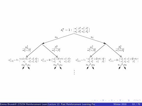
Bayes-Adaptive Bernoulli Bandits
Start with Beta(αa, βa) priorover reward function Ra
Each time a is selected,update posterior for Ra
Beta(αa + 1, βa) if r = 0Beta(αa, βa + 1) if r = 1
This defines transitionfunction P for theBayes-adaptive MDP
Information state (α, β)corresponds to reward modelBeta(α, β)
Each state transitioncorresponds to a Bayesianmodel update
Emma Brunskill (CS234 Reinforcement Learning. )Lecture 12: Fast Reinforcement Learning Part II 63 Winter 2018 52 / 70
Emma Brunskill (CS234 Reinforcement Learning. )Lecture 12: Fast Reinforcement Learning Part II 64 Winter 2018 53 / 70
Gittins Indices for Bernoulli Bandits
Bayes-adaptive MDP can be solved by dynamic programming
The solution is known as the Gittins index
Exact solution to Bayes-adaptiev MDP is typically intractable;information state space is too large
Recent idea: apply simulation-based search (Guez et al. 2012, 2013)
Forward search in information state spaceUsing simulations from current information state
Emma Brunskill (CS234 Reinforcement Learning. )Lecture 12: Fast Reinforcement Learning Part II 65 Winter 2018 54 / 70
Table of Contents
1 Metrics for evaluating RL algorithms
2 Principles for RL Exploration
3 Probability Matching
4 Information State Search
5 MDPs
6 Principles for RL Exploration
7 Metrics for evaluating RL algorithms
Emma Brunskill (CS234 Reinforcement Learning. )Lecture 12: Fast Reinforcement Learning Part II 66 Winter 2018 55 / 70

Principles for Strategic Exploration
The sample principles for exploration/exploitation apply to MDPs
Naive ExplorationOptimistic InitializationOptimism in the Face of UncertaintyProbability MatchingInformation State Search
Emma Brunskill (CS234 Reinforcement Learning. )Lecture 12: Fast Reinforcement Learning Part II 67 Winter 2018 56 / 70
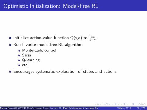
Optimistic Initialization: Model-Free RL
Initialize action-value function Q(s,a) to rmax1−γ
Run favorite model-free RL algorithm
Monte-Carlo controlSarsaQ-learningetc.
Encourages systematic exploration of states and actions
Emma Brunskill (CS234 Reinforcement Learning. )Lecture 12: Fast Reinforcement Learning Part II 68 Winter 2018 57 / 70

Optimistic Initialization: Model-Based RL
Construct an optimistic model of the MDP
Initialize transitions to go to terminal state with rmax reward
Solve optimistic MDP by favorite planning algorithm
Encourages systematic exploration of states and actions
e.g. RMax algorithm (Brafman and Tennenholtz)
Emma Brunskill (CS234 Reinforcement Learning. )Lecture 12: Fast Reinforcement Learning Part II 69 Winter 2018 58 / 70

UCB: Model-Based RL
Maximize UCB on action-value function Qπ(s, a)
at = arg maxa∈A
Q(st , a) + U(st , a)
Estimate uncertainty in policy evaluation (easy)Ignores uncertainty from policy improvement
Maximize UCB on optimal action-value function Q∗(s, a)
at = arg maxa∈A
Q(st , a) + U1(st , a) + U2(st , a)
Estimate uncertainty in policy evaluation (easy)plus uncertainty from policy improvement (hard)
Emma Brunskill (CS234 Reinforcement Learning. )Lecture 12: Fast Reinforcement Learning Part II 70 Winter 2018 59 / 70

Bayesian Model-Based RL
Maintain posterior distribution over MDP models
Estimate both transition and rewards, p[P,R | ht ], whereht = (s1, a1, r1, . . . , st) is the history
Use posterior to guide exploration
Upper confidence bounds (Bayesian UCB)Probability matching (Thompson sampling)
Emma Brunskill (CS234 Reinforcement Learning. )Lecture 12: Fast Reinforcement Learning Part II 71 Winter 2018 60 / 70
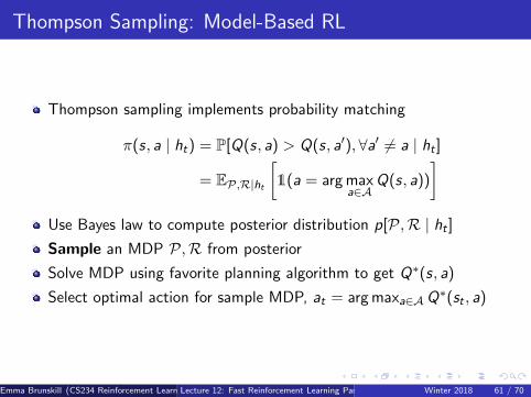
Thompson Sampling: Model-Based RL
Thompson sampling implements probability matching
π(s, a | ht) = P[Q(s, a) > Q(s, a′),∀a′ 6= a | ht ]
= EP,R|ht
[1(a = arg max
a∈AQ(s, a))
]Use Bayes law to compute posterior distribution p[P,R | ht ]Sample an MDP P,R from posterior
Solve MDP using favorite planning algorithm to get Q∗(s, a)
Select optimal action for sample MDP, at = arg maxa∈AQ∗(st , a)
Emma Brunskill (CS234 Reinforcement Learning. )Lecture 12: Fast Reinforcement Learning Part II 72 Winter 2018 61 / 70
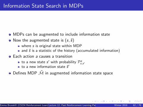
Information State Search in MDPs
MDPs can be augmented to include information state
Now the augmented state is (s, s)
where s is original state within MDPand s is a statistic of the history (accumulated information)
Each action a causes a transition
to a new state s ′ with probability Pas,s′
to a new information state s ′
Defines MDP M in augmented information state space
Emma Brunskill (CS234 Reinforcement Learning. )Lecture 12: Fast Reinforcement Learning Part II 73 Winter 2018 62 / 70

Bayes Adaptive MDP
Posterior distribution over MDP model is an information state
st = P[P,R | ht ]
Augmented MDP over (s, s) is called Bayes-adaptive MDP
Solve this MDP to find optimal exploration/exploitation trade-off(with respect to prior)
However, Bayes-adaptive MDP is typically enormous
Simulation-based search has proven effective (Guez et al, 2012, 2013)
Emma Brunskill (CS234 Reinforcement Learning. )Lecture 12: Fast Reinforcement Learning Part II 74 Winter 2018 63 / 70

Table of Contents
1 Metrics for evaluating RL algorithms
2 Principles for RL Exploration
3 Probability Matching
4 Information State Search
5 MDPs
6 Principles for RL Exploration
7 Metrics for evaluating RL algorithms
Emma Brunskill (CS234 Reinforcement Learning. )Lecture 12: Fast Reinforcement Learning Part II 75 Winter 2018 64 / 70
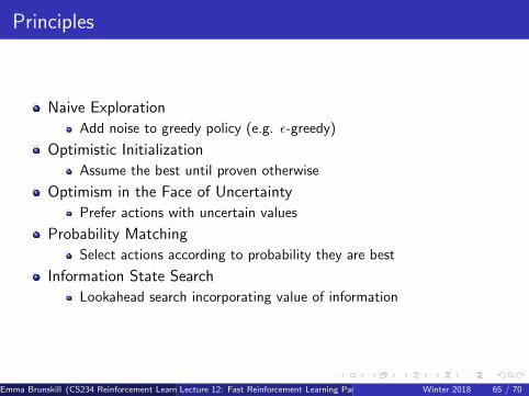
Principles
Naive Exploration
Add noise to greedy policy (e.g. ε-greedy)
Optimistic Initialization
Assume the best until proven otherwise
Optimism in the Face of Uncertainty
Prefer actions with uncertain values
Probability Matching
Select actions according to probability they are best
Information State Search
Lookahead search incorporating value of information
Emma Brunskill (CS234 Reinforcement Learning. )Lecture 12: Fast Reinforcement Learning Part II 76 Winter 2018 65 / 70

Generalization and Strategic Exploration
Active area of ongoing research: combine generalization & strategicexploration
Many approaches are grounded by principles outlined here
Some examples:
Optimism under uncertainty: Bellemare et al. NIPS 2016; Ostrovski etal. ICML 2017; Tang et al. NIPS 2017Probability matching: Osband et al. NIPS 2016; Mandel et al. IJCAI2016
Emma Brunskill (CS234 Reinforcement Learning. )Lecture 12: Fast Reinforcement Learning Part II 77 Winter 2018 66 / 70
Table of Contents
1 Metrics for evaluating RL algorithms
2 Principles for RL Exploration
3 Probability Matching
4 Information State Search
5 MDPs
6 Principles for RL Exploration
7 Metrics for evaluating RL algorithms
Emma Brunskill (CS234 Reinforcement Learning. )Lecture 12: Fast Reinforcement Learning Part II 78 Winter 2018 67 / 70

Performance Criteria of RL Algorithms
Empirical performance
Convergence (to something ...)
Asymptotic convergence to optimal policy
Finite sample guarantees: probably approximately correct
Regret (with respect to optimal decisions)
Optimal decisions given information have available
PAC uniform (Dann, Tor, Brunskill NIPS 2017): stronger criteria,directly provides both PAC and regret bounds
Emma Brunskill (CS234 Reinforcement Learning. )Lecture 12: Fast Reinforcement Learning Part II 79 Winter 2018 68 / 70
Summary: What You Are Expected to Know
Define the tension of exploration and exploitation in RL and why thisdoes not arise in supervised or unsupervised learning
Be able to define and compare different criteria for ”good”performance (empirical, convergence, asymptotic, regret, PAC)
Be able to map algorithms discussed in detail in class to theperformance criteria they satisfy
Emma Brunskill (CS234 Reinforcement Learning. )Lecture 12: Fast Reinforcement Learning Part II 80 Winter 2018 69 / 70

Class Structure
Last time: Exploration and Exploitation Part I
This time: Exploration and Exploitation Part II
Next time: Batch RL
Emma Brunskill (CS234 Reinforcement Learning. )Lecture 12: Fast Reinforcement Learning Part II 81 Winter 2018 70 / 70
![Lecture 13: Fast Reinforcement Learning =1[1]With …web.stanford.edu/class/cs234/slides/lecture13_postclass.pdfThen after observed a reward r 2f0;1gthen updated posterior over is](https://static.fdocuments.in/doc/165x107/5d341b9b88c993b2278b631b/lecture-13-fast-reinforcement-learning-11with-web-after-observed-a-reward-r.jpg)


![Lecture 12: Fast Reinforcement Learning [1]With some ... · Lecture 12: Fast Reinforcement Learning 1 Emma Brunskill CS234 Reinforcement Learning Winter 2020 1With some slides derived](https://static.fdocuments.in/doc/165x107/5ed82f150fa3e705ec0dfdfc/lecture-12-fast-reinforcement-learning-1with-some-lecture-12-fast-reinforcement.jpg)


![Lecture 16: MCTS =1[1]With many slides from or derived ... · Lecture 16: MCTS 1 Emma Brunskill CS234 Reinforcement Learning. Winter 2018 1With many slides from or derived from David](https://static.fdocuments.in/doc/165x107/5e21ad4169fe1301e360183e/lecture-16-mcts-11with-many-slides-from-or-derived-lecture-16-mcts-1-emma.jpg)
![Lecture 16: MCTS =1[1]With many slides from or …...Lecture 16: MCTS 1 Emma Brunskill CS234 Reinforcement Learning. Winter 2018 1With many slides from or derived from David Silver](https://static.fdocuments.in/doc/165x107/5f31d9cdf90e4815e078b7d3/lecture-16-mcts-11with-many-slides-from-or-lecture-16-mcts-1-emma-brunskill.jpg)
![Lecture 12: Fast Reinforcement Learning [1]With …web.stanford.edu/class/cs234/slides/lecture12_postclass.pdfLecture 12: Fast Reinforcement Learning 1 Emma Brunskill CS234 Reinforcement](https://static.fdocuments.in/doc/165x107/5ea9dceb336dde7b5c510cf2/lecture-12-fast-reinforcement-learning-1with-web-lecture-12-fast-reinforcement.jpg)


