Lecture 11 Transmission Lines - Purdue University

Lecture 11

Transmission Lines

Transmission lines represent one of the most important electromagnetic technologies. Thereason being that they can be described by simple theory, similar to circuit theory. As such,the theory is within the grasp of most practicing electrical engineers. Moreover, transmissionline theory fills the gap in the physics of circuit theory: Circuit theory alone cannot describewave phenomena, but when circuit theory is augmented with transmission line theory, wavephenomena with its corresponding wave physics start to emerge.

Even though circuit theory has played an indispensable role in the development of thecomputer chip industry, it has to be embellished by transmission line theory, so that high-speed circuits can be designed. Retardation effect, which causes time delay, clock skew, andphase shift, can be modeled simply using transmission lines. Nowadays, commercial circuitsolver software have the capability of including transmission line as an element in modeling.

111

112 Electromagnetic Field Theory

11.1 Transmission Line Theory

Figure 11.1: Various kinds of transmission lines. Schematically, all of them can be modeledby two parallel wires.

Transmission lines were the first electromagnetic waveguides ever invented. The were drivenby the needs in telegraphy technology. It is best to introduce transmission line theory fromthe viewpoint of circuit theory, which is elegant and one of the simplest theories of electricalengineering. This theory is also discussed in many textbooks and lecture notes. Transmissionlines are so important in modern day electromagnetic engineering, that most engineeringelectromagnetics textbooks would be incomplete without introducing the topics related tothem [31,32,44,50,54,65,79,83,85,86].

Circuit theory is robust and is not sensitive to the detail shapes of the components in-volved such as capacitors or inductors. Moreover, many transmission line problems cannotbe analyzed simply when the full form of Maxwell’s equations is used,1 but approximatesolutions can be obtained using circuit theory in the long-wavelength limit. We shall showthat circuit theory is an approximation of electromagnetic field theory when the wavelengthis very long: the longer the wavelength, the better is the approximation [50].

Examples of transmission lines are shown in Figure 11.1. The symbol for a transmissionline is usually represented by two pieces of parallel wires, but in practice, these wires neednot be parallel as showin in Figure 11.2.

1Usually called full-wave analysis.

Transmission Lines 113

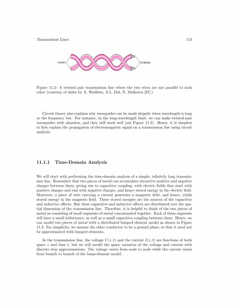
Figure 11.2: A twisted pair transmission line where the two wires are not parallel to eachother (courtesy of slides by A. Wadhwa, A.L. Dal, N. Malhotra [87].)

Circuit theory also explains why waveguides can be made sloppily when wavelength is longor the frequency low. For instance, in the long-wavelength limit, we can make twisted-pairwaveguides with abandon, and they still work well (see Figure 11.2). Hence, it is simplestto first explain the propagation of electromagnetic signal on a transmission line using circuitanalysis.

11.1.1 Time-Domain Analysis

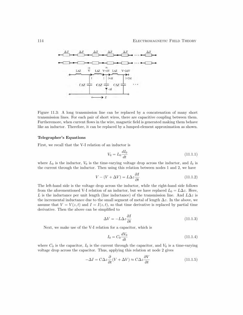
We will start with performing the time-domain analysis of a simple, infinitely long transmis-sion line. Remember that two pieces of metal can accumulate attractive positive and negativecharges between them, giving rise to capacitive coupling, with electric fields that start withpositive charges and end with negative charges, and hence stored energy in the electric field.Moreover, a piece of wire carrying a current generates a magnetic field, and hence, yieldsstored energy in the magnetic field. These stored energies are the sources of the capacitiveand inductive effects. But these capacitive and inductive effects are distributed over the spa-tial dimension of the transmission line. Therefore, it is helpful to think of the two pieces ofmetal as consisting of small segments of metal concatenated together. Each of these segmentswill have a small inductance, as well as a small capacitive coupling between them. Hence, wecan model two pieces of metal with a distributed lumped element model as shown in Figure11.3. For simplicity, we assume the other conductor to be a ground plane, so that it need notbe approximated with lumped elements.

In the transmission line, the voltage V (z, t) and the current I(z, t) are functions of bothspace z and time t, but we will model the space variation of the voltage and current withdiscrete step approximations. The voltage varies from node to node while the current variesfrom branch to branch of the lump-element model.


Figure 11.3: A long transmission line can be replaced by a concatenation of many shorttransmission lines. For each pair of short wires, there are capacitive coupling between them.Furtheremore, when current flows in the wire, magnetic field is generated making them behavelike an inductor. Therefore, it can be replaced by a lumped-element approximation as shown.

Telegrapher’s Equations

First, we recall that the V-I relation of an inductor is

V0 = L0dI0dt

(11.1.1)

where L0 is the inductor, V0 is the time-varying voltage drop across the inductor, and I0 isthe current through the inductor. Then using this relation between nodes 1 and 2, we have

V − (V + ∆V ) = L∆z∂I

∂t(11.1.2)

The left-hand side is the voltage drop across the inductor, while the right-hand side followsfrom the aforementioned V-I relation of an inductor, but we have replaced L0 = L∆z. Here,L is the inductance per unit length (line inductance) of the transmission line. And L∆z isthe incremental inductance due to the small segment of metal of length ∆z. In the above, weassume that V = V (z, t) and I = I(z, t), so that time derivative is replaced by partial timederivative. Then the above can be simplified to

∆V = −L∆z∂I

∂t(11.1.3)

Next, we make use of the V-I relation for a capacitor, which is

I0 = C0dV0

dt(11.1.4)

where C0 is the capacitor, I0 is the current through the capacitor, and V0 is a time-varyingvoltage drop across the capacitor. Thus, applying this relation at node 2 gives

−∆I = C∆z∂

∂t(V + ∆V ) ≈ C∆z

∂V

∂t(11.1.5)


where C is the capacitance per unit length, and C∆z is the incremental capacitance betweenthe small piece of metal and the ground plane. In the above, we have used Kirchhoff currentlaw to surmise that the current through the capacitor is−∆I, where ∆I = I(z+∆z, t)−I(z, t).In the last approximation in (11.1.5), we have dropped a term involving the product of ∆zand ∆V , since it will be very small or second order in magnitude.

In the limit when ∆z → 0, one gets from (11.1.3) and (11.1.5) that

∂V (z, t)

∂z= −L∂I(z, t)

∂t(11.1.6)

∂I(z, t)

∂z= −C ∂V (z, t)

∂t(11.1.7)

The above are the telegrapher’s equations.2 They are two coupled first-order equations,and can be converted into second-order equations easily. Therefore,

∂2V

∂z2− LC ∂

2V

∂t2= 0 (11.1.8)

∂2I

∂z2− LC ∂

2I

∂t2= 0 (11.1.9)

The above are wave equations that we have previously studied, where the velocity of the waveis given by

v =1√LC

(11.1.10)

Furthermore, if we assume that

V (z, t) = V0f+(z − vt), I(z, t) = I0f+(z − vt) (11.1.11)

corresponding to a right-traveling wave, they can be verified to satisfy (11.1.6) and (11.1.7)by back substitution.

Consequently, we can easily show that

V (z, t)

I(z, t)=

√L

C= Z0 (11.1.12)

where Z0 is the characteristic impedance of the transmission line. The above ratio is onlytrue for one-way traveling wave, in this case, one that propagates in the +z direction.

For a wave that travels in the negative z direction, we can let,

V (z, t) = V0f−(z + vt), I(z, t) = I0f−(z + vt) (11.1.13)

one can easily show that

V (z, t)

I(z, t)= −

√L

C= −Z0 (11.1.14)

2They can be thought of as the distillation of the Faraday’s law and Ampere’s law from Maxwell’s equationswithout the source term. Their simplicity gives them an important role in engineering electromagnetics.


Time-domain analysis is very useful for transient analysis of transmission lines, especiallywhen nonlinear elements are coupled to the transmission line.3 Another major strengthof transmission line model is that it is a simple way to introduce time-delay (also calledretardation) in a simple circuit model.4

Time delay is a wave propagation effect, and it is harder to incorporate into circuit theoryor a pure circuit model consisting of R, L, and C only. In circuit theory, where the wavelengthis assumed very long, Laplace’s equation is usually solved, which is equivalent to Helmholtzequation with infinite wave velocity, namely,

limc→∞

∇2Φ(r) +ω2

c2Φ(r) = 0 =⇒ ∇2Φ(r) = 0 (11.1.15)

Hence, events in Laplace’s equation happen instantaneously. In other words, circuit theoryassumes that the velocity of the wave is infinite, and there is no retardation effect. Thisis only true or a good approximation when the size of the structure is small compared towavelength.

11.1.2 Frequency-Domain Analysis–the Power of Phasor TechniqueAgain!

Frequency domain analysis is very popular as it makes the transmission line equations verysimple–one just replace ∂/∂t → jω. Moreover, generalization to a lossy system is quitestraight forward. Furthermore, for linear time invariant systems, the time-domain signals canbe obtained from the frequency-domain data by performing a Fourier inverse transform sincephasors and Fourier transforms of a time variable are just related to each other by a constant.

The telegrapher’s equations (11.1.6) and (11.1.7) then in frequency domain become

d

dzV (z, ω) = −jωLI(z, ω) (11.1.16)

d

dzI(z, ω) = −jωCV (z, ω) (11.1.17)

The corresponding Helmholtz equations are then

d2V

dz2+ ω2LCV = 0 (11.1.18)

d2I

dz2+ ω2LCI = 0 (11.1.19)

The above are second ordinary differential equations, and the general solutions to the aboveare

V (z) = V+e−jβz + V−e

jβz (11.1.20)

I(z) = I+e−jβz + I−e

jβz (11.1.21)

3Remember that we can only use frequency domain technique or Fourier transform for linear time-invariantsystems.

4By a simple circuit model, we mean a model that has lumped elements such as R, L, and C as well as atransmission line element.


where β = ω√LC. This is similar to what we have seen previously for plane waves in the

one-dimensional wave equation in free space, where

Ex(z) = E0+e−jk0z + E0−e

jk0z (11.1.22)

where k0 = ω√µ0ε0. We see much similarity between (11.1.20), (11.1.21), and (11.1.22).

To see the solution in the time domain, we let the phasor V± = |V±|ejφ± in (11.1.20),and the voltage signal above can then be converted back to the time domain using the keyformula in phasor technique as

V (z, t) = <e{V (z, ω)ejωt} (11.1.23)

= |V+| cos(ωt− βz + φ+) + |V−| cos(ωt+ βz + φ−) (11.1.24)

As can be seen, the first term corresponds to a right-traveling wave, while the second term isa left-traveling wave.

Furthermore, if we assume only a one-way traveling wave to the right by letting V− =I− = 0, then it can be shown that, for a right-traveling wave, using (11.1.16) or (11.1.17)

V (z)

I(z)=V+

I+=

√L

C= Z0 (11.1.25)

where Z0 is the characteristic impedance. Since Z0 is real, it implies that V (z) and I(z) arein phase.

Similarly, applying the same process for a left-traveling wave only, by letting V+ = I+ = 0,then

V (z)

I(z)=V−I−

= −√L

C= −Z0 (11.1.26)

In other words, for the left-traveling waves, the voltage and current are 180 ◦ out of phase.

11.2 Lossy Transmission Line

Figure 11.4: In a lossy transmission line, series resistance can be added to the series induc-tance, and the shunt conductance can be added to the shun susceptance of the capacitor.However, this problem is homomorphic to the lossless case in the frequency domain.


The power of frequency domain analysis is revealed in the study of lossy transmission lines.The previous analysis, which is valid for lossless transmission line, can be easily generalizedto the lossy case in the frequency domain. In using frequency domain and phasor technique,impedances will become complex numbers as shall be shown.

To include loss, we use the lumped-element model as shown in Figure 11.4. One thing tonote is that jωL is actually the series line impedance of the lossless transmission line, whilejωC is the shunt line admittance of the same line. First, we can rewrite the expressions forthe telegrapher’s equations in (11.1.16) and (11.1.17) in terms of series line impedance andshunt line admittance to arrive at

d

dzV = −ZI (11.2.1)

d

dzI = −Y V (11.2.2)

where Z = jωL and Y = jωC. The above can be easily generalized to the lossy case as shallbe shown.

The geometry in Figure 11.4 is topologically similar to, or homomorphic5 to the losslesscase in Figure 11.3. Hence, when lossy elements are added in the geometry, we can surmisethat the corresponding telegrapher’s equations are similar to those above. But to include loss,we need only to generalize the series line impedance and shunt admittance from the losslesscase to lossy case as follows:

Z = jωL→ Z = jωL+R (11.2.3)

Y = jωC → Y = jωC +G (11.2.4)

where R is the series line resistance, and G is the shunt line conductance, and now Z andY are the series impedance and shunt admittance, (which are complex number rather thanbeing pure imaginary), respectively. Then, the corresponding Helmholtz equations are

d2V

dz2− ZY V = 0 (11.2.5)

d2I

dz2− ZY I = 0 (11.2.6)

or

d2V

dz2− γ2V = 0 (11.2.7)

d2I

dz2− γ2I = 0 (11.2.8)

where γ2 = ZY , or that one can also think of γ2 = −β2 by comparing with (11.1.18) and(11.1.19). Then the above is homomorphic to the lossless case except that now, β is a complex

5A math term for “similar in math structure”. The term is even used in computer science describing aemerging field of homomorphic computing.


number, indicating that the field is decaying as it propagates. As before, the above are secondorder one-dimensional Helmholtz equations where the general solutions are

V (z) = V+e−γz + V−e

γz (11.2.9)

I(z) = I+e−γz + I−e

γz (11.2.10)

and

γ =√ZY =

√(jωL+R)(jωC +G) = jβ (11.2.11)

Here, β = β′ − jβ′′ is now a complex number. In other words,

e−γz = e−jβ′z−β′′z

is an oscillatory and decaying wave. Or focusing on the voltage case,

V (z) = V+e−β′′z−jβ′z + V−e

β′′z+jβ′z (11.2.12)

Again, letting V± = |V±|ejφ± , the above can be converted back to the time domain as

V (z, t) = <e{V (z, ω)ejωt} (11.2.13)

= |V+|e−β′′z cos(ωt− β′z + φ+) + |V−|eβ

′′z cos(ωt+ β′z + φ−) (11.2.14)

The first term corresponds to a decaying wave moving to the right while the second term isalso a decaying wave but moving to the left. When there is no loss, or R = G = 0, and from(11.2.11), we retrieve the lossless case where β′′ = 0 and γ = jβ = jω

√LC.

Notice that for the lossy case, the characteristic impedance, which is the ratio of thevoltage to the current for a one-way wave, can similarly be derived using homomorphism:

Z0 =V+

I+= −V−

I−=

√L

C=

√jωL

jωC→ Z0 =

√Z

Y=

√jωL+R

jωC +G(11.2.15)

The above Z0 is manifestly a complex number. Here, Z0 is the ratio of the phasors of theone-way traveling waves, and apparently, their current phasor and the voltage phasor will notbe in phase for lossy transmission line.

In the absence of loss, the above again becomes

Z0 =

√L

C(11.2.16)

the characteristic impedance for the lossless case previously derived.

Lecture 11 Transmission Lines - Purdue University

Documents

Transcript of Lecture 11 Transmission Lines - Purdue University