Lecture 11: Shock Tube Techniques/Applications Lecture Notes/Hanson... · Lecture 11: Shock Tube...
39
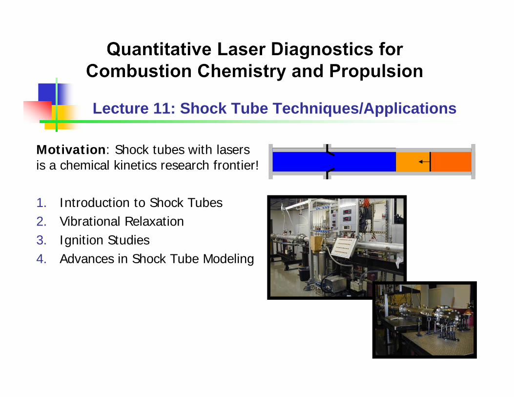
Lecture 11: Shock Tube Techniques/Applications Motivation: Shock tubes with lasers is a chemical kinetics research frontier! 1. Introduction to Shock Tubes 2. Vibrational Relaxation 3. Ignition Studies 4. Advances in Shock Tube Modeling
Transcript of Lecture 11: Shock Tube Techniques/Applications Lecture Notes/Hanson... · Lecture 11: Shock Tube...
Lecture 11: Shock Tube Techniques/Applications
Motivation: Shock tubes with lasers is a chemical kinetics research frontier!
1. Introduction to Shock Tubes2. Vibrational Relaxation3. Ignition Studies4. Advances in Shock Tube Modeling
2
1. Introduction to Shock Tubes
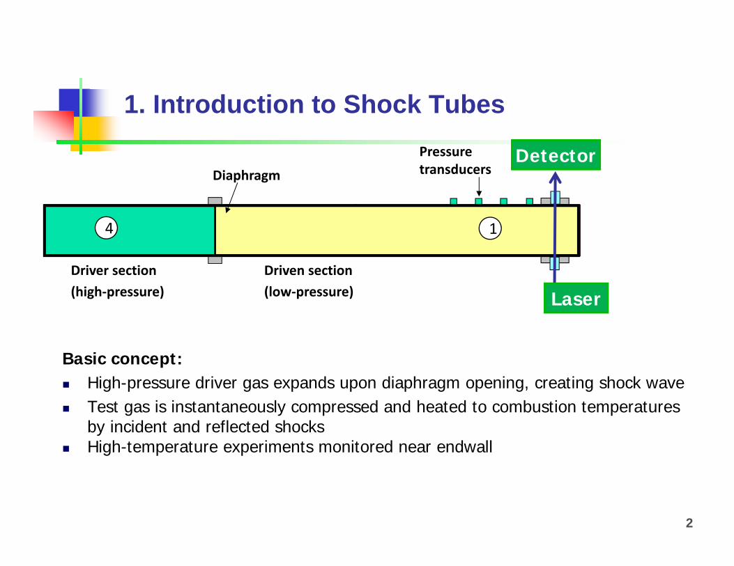
Basic concept: High-pressure driver gas expands upon diaphragm opening, creating shock wave Test gas is instantaneously compressed and heated to combustion temperatures
by incident and reflected shocks High-temperature experiments monitored near endwall
High P Low P1
Diaphragm
Pressure transducers
52
Driver section(high‐pressure)
Driven section(low‐pressure)
4 1
Detector
Laser

3
1. Introduction to Shock Tubes
Basic concept: High-pressure driver gas expands upon diaphragm opening creating shock wave Test gas is instantaneously compressed and heated to combustion temperatures
from incident and reflected shocks High-temperature experiments monitored at endwall
High P Low P1
Diaphragm
Pressure transducers
Incident Shock
Reflected shock
52
Driver section(high‐pressure)
Driven section(low‐pressure)
Detector
Laser
4
1. Introduction to Shock Tubes
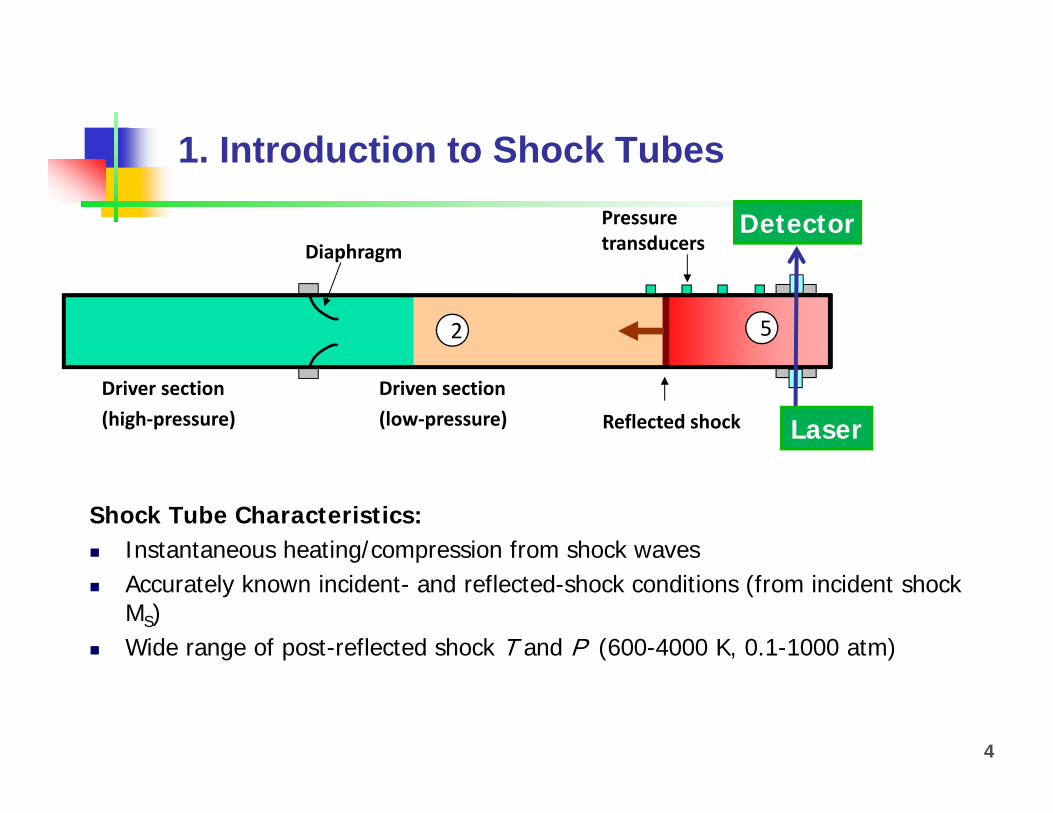
Shock Tube Characteristics: Instantaneous heating/compression from shock waves Accurately known incident- and reflected-shock conditions (from incident shock
MS) Wide range of post-reflected shock T and P (600-4000 K, 0.1-1000 atm)
High P Low P1
Diaphragm
Pressure transducers
Reflected shock
52
Driver section(high‐pressure)
Driven section(low‐pressure)
Detector
Laser
5
1. Introduction to Shock Tubes
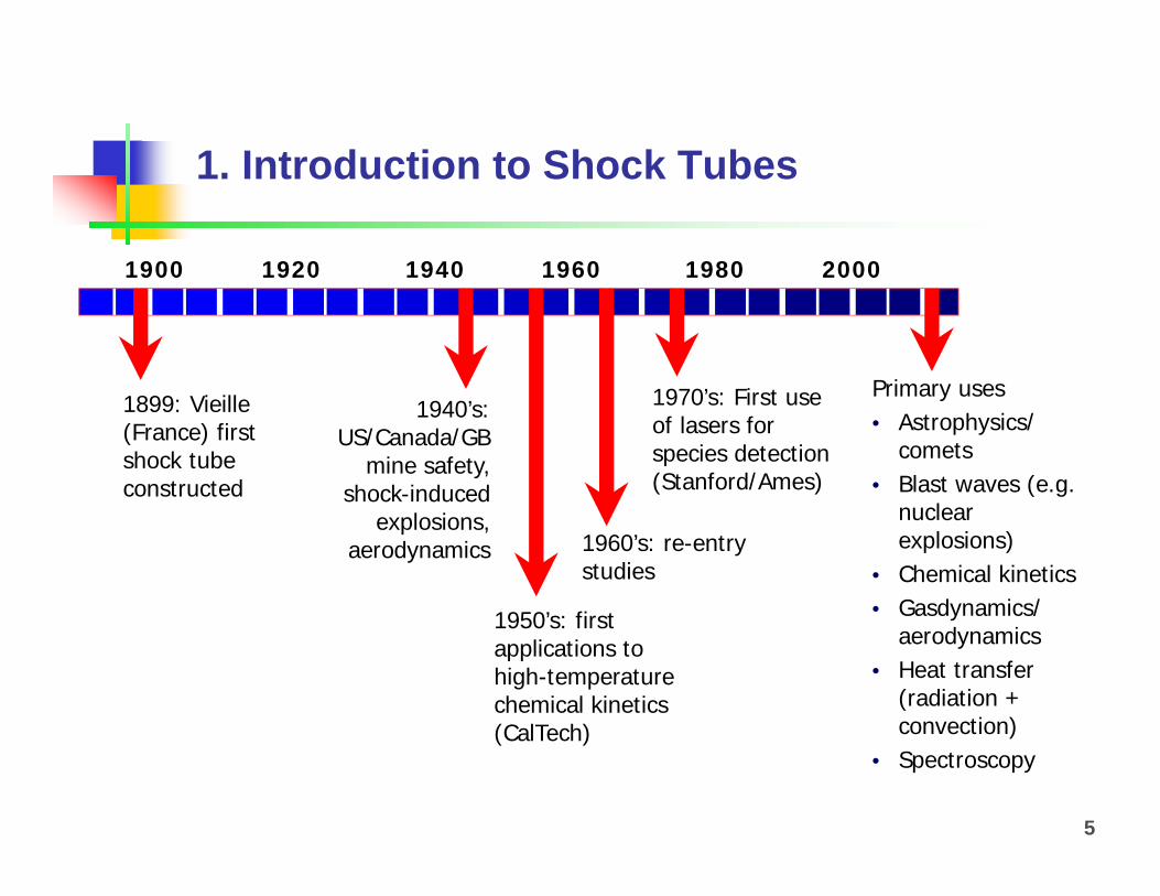
Primary uses• Astrophysics/
comets• Blast waves (e.g.
nuclear explosions)
• Chemical kinetics• Gasdynamics/
aerodynamics• Heat transfer
(radiation + convection)
• Spectroscopy
1900 1920 1940 1960 1980 2000
1899: Vieille (France) first shock tube constructed
1940’s: US/Canada/GB
mine safety, shock-induced
explosions, aerodynamics
1950’s: first applications to high-temperature chemical kinetics (CalTech)
1960’s: re-entry studies
1970’s: First use of lasers for species detection (Stanford/Ames)
6
p1T1ρ1v1 = 0
Vs
1. Introduction to Shock Tubes
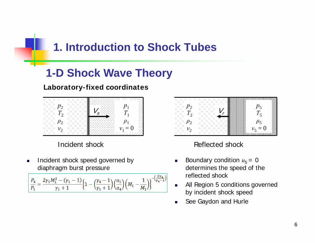
Incident shock speed governed by diaphragm burst pressure
Boundary condition u5 = 0 determines the speed of the reflected shock
All Region 5 conditions governed by incident shock speed
See Gaydon and Hurle
p2T2ρ2v2
Incident shock Reflected shock
Vr
Laboratory-fixed coordinates
p2T2ρ2v2
p5T5ρ5v5 = 0
1-D Shock Wave Theory

7
1. Introduction to Shock Tubes
P2/P1 P5/P2 WR/WS2.95 10 4.95 2.62 1.76 3.82 2.82 0.4236.56 50 7.12 9.31 2.28 5.37 3.11 0.351 8.00 2.29 6.00 3.50 0.333
2.87 10 4.22 3.42 1.94 2.92 2.17 0.5896.34 50 5.54 13.4 2.37 3.72 2.31 0.517 6.00 2.40 4.00 2.50 0.500
7/5
5/3
2 4 6 8 101
10
100
T5/T1 ( T5/T1 ( T2/T1 ( T2/T1 (
T 2/T1 (
or T
5/T1)
MS
2 4 6 8 101
10
100
P5/P1 ( P5/P1 ( P2/P1 ( P2/P1 (
P 2/P1 (o
r P5/P
1)
MS
Shock Jump Values
8
1. Introduction to Shock Tubes
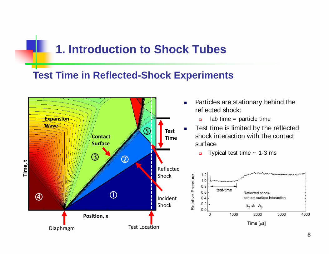
Particles are stationary behind the reflected shock: lab time = particle time
Test time is limited by the reflected shock interaction with the contact surface Typical test time ~ 1-3 ms
Diaphragm
Position, x
Time, t
Expansion Wave
IncidentShock
ReflectedShock
Test Location
ContactSurface
TestTime
Test Time in Reflected-Shock Experiments
a2 a3
9
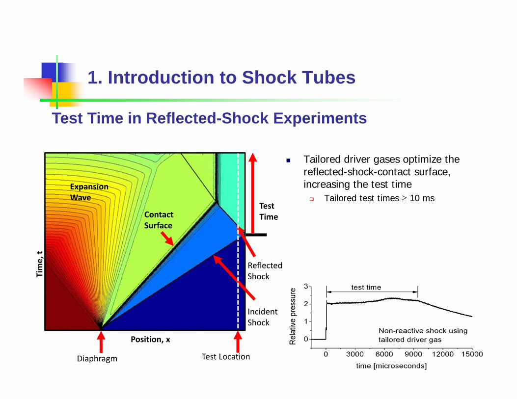
Tailored driver gases optimize the reflected-shock-contact surface, increasing the test time Tailored test times 10 ms
1. Introduction to Shock Tubes
Diaphragm
Position, x
Time, t
Expansion Wave
IncidentShock
ReflectedShock
Test Location
ContactSurface
TestTime
Test Time in Reflected-Shock Experiments
10
2. Vibrational Relaxation
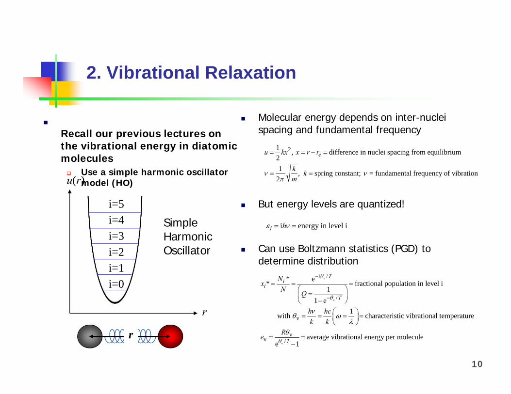
Recall our previous lectures on the vibrational energy in diatomic molecules Use a simple harmonic oscillator
model (HO)
Molecular energy depends on inter-nuclei spacing and fundamental frequency
But energy levels are quantized!
Can use Boltzmann statistics (PGD) to determine distribution
i energy in level ii h Simple Harmonic Oscillator
i=5i=4i=3i=2i=1i=0
r
u(r)
r
21 , difference in nuclei spacing from equilibrium21 , spring constant; = fundamental frequency of vibration
2
eu kx x r r
k km
v
v
v
i /
/
v
vv /
* e* fractional population in level i1
1 e1 with characteristic vibrational temperature
average vibrational energy per moleculee 1
Ti
i
T
T
NxN Q
h hck k
Re

11
Vibrational energy distribution function (from Boltzmann statistics)
More molecules in lower vibrational levels than in high vibrational levels
Higher energy levels get populated at higher temperatures
Temperature refers to the vibrational temperature (T = Tv), the same as translational temperature in vibrational equilibrium
If Tv = Ttrans then vibrational energy transfer will occur until the system reaches equilibrium→ vibra onal relaxa on!
2. Vibrational Relaxation
v
v
i /
/
* e* fractional population in level i1
1 e
Ti
i
T
NxN Q
0 1 2 3 41E-3
0.01
0.1
1
vibrational level, i
T=300 K
high T
popu
latio
n, x
i*
12
2. Vibrational Relaxation
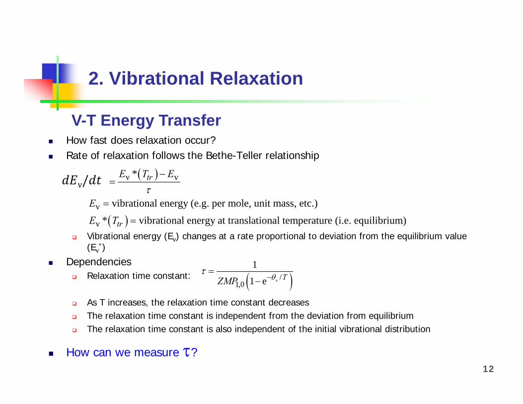
How fast does relaxation occur? Rate of relaxation follows the Bethe-Teller relationship
.
Vibrational energy (Ev) changes at a rate proportional to deviation from the equilibrium value (Ev
*)
Dependencies Relaxation time constant:
As T increases, the relaxation time constant decreases The relaxation time constant is independent from the deviation from equilibrium The relaxation time constant is also independent of the initial vibrational distribution
How can we measure ?
v vv
v
v
*
vibrational energy (e.g. per mole, unit mass, etc.)* vibrational energy at translational temperature (i.e. equilibrium)
tr
tr
E T EEt
EE T
v /1,0
1
1 e TZMP
V-T Energy Transfer
v/
13
2. Vibrational Relaxation
T
t
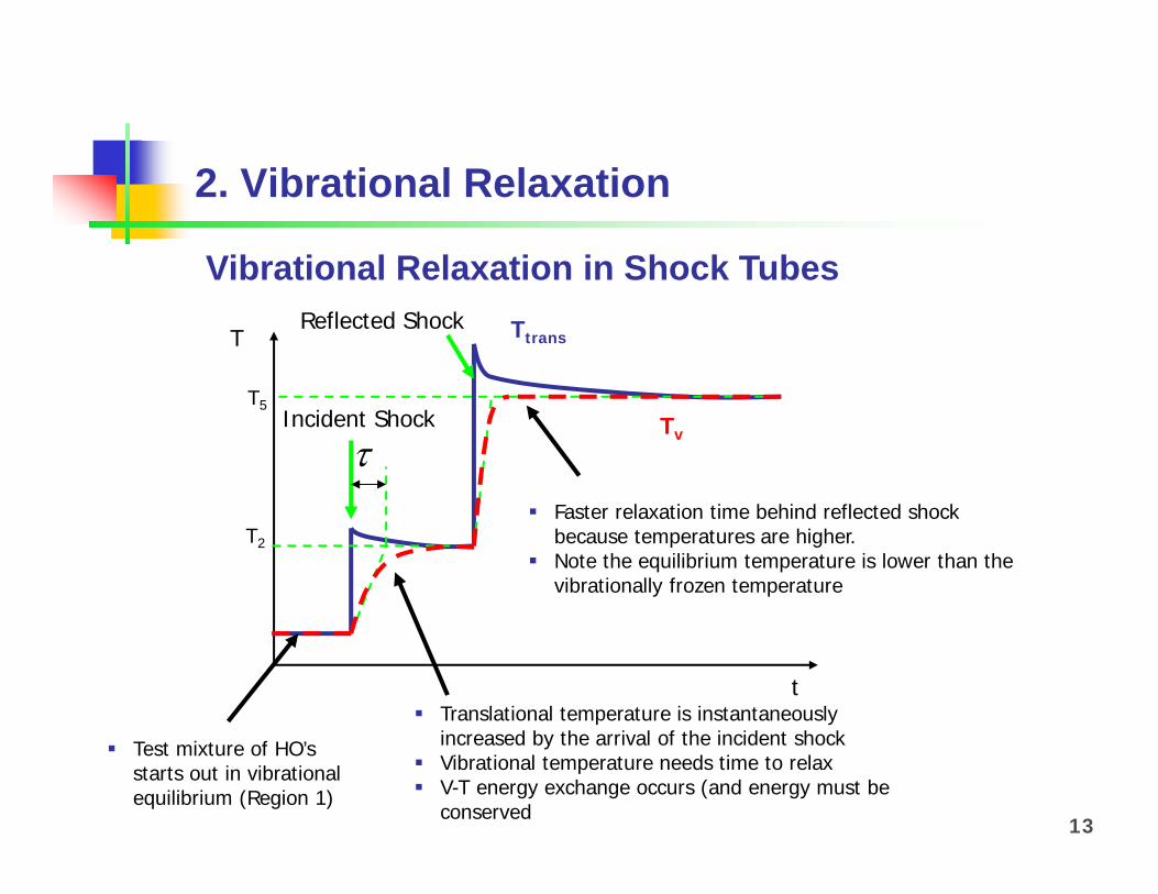
Test mixture of HO’s starts out in vibrational equilibrium (Region 1)
Translational temperature is instantaneously increased by the arrival of the incident shock
Vibrational temperature needs time to relax V-T energy exchange occurs (and energy must be
conserved
Faster relaxation time behind reflected shock because temperatures are higher.
Note the equilibrium temperature is lower than the vibrationally frozen temperature
Ttrans
TvIncident Shock
Reflected Shock
T2
T5
Vibrational Relaxation in Shock Tubes
14
2. Vibrational Relaxation
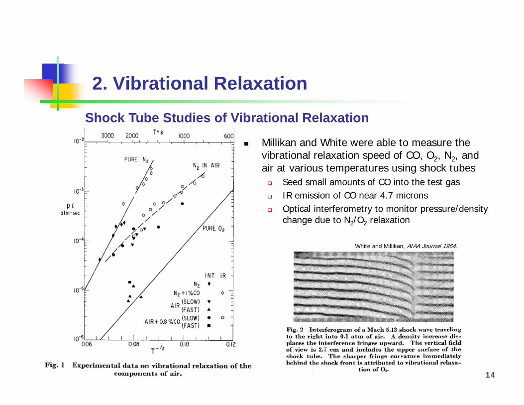
White and Millikan, AIAA Journal 1964.
Millikan and White were able to measure the vibrational relaxation speed of CO, O2, N2, and air at various temperatures using shock tubes Seed small amounts of CO into the test gas IR emission of CO near 4.7 microns Optical interferometry to monitor pressure/density
change due to N2/O2 relaxation
Shock Tube Studies of Vibrational Relaxation
2. Vibrational Relaxation
15
• Modern Experiments with Laser Diagnostics
Goal:• High-temperature O2 vibration relaxation rates
Experimental Strategy:• Shock heat highly diluted mixtures of O2 in Ar• New diagnostic (MIRA laser) to measure O2 in deep UV
(Schumann-Runge) at 206 to 245 nm
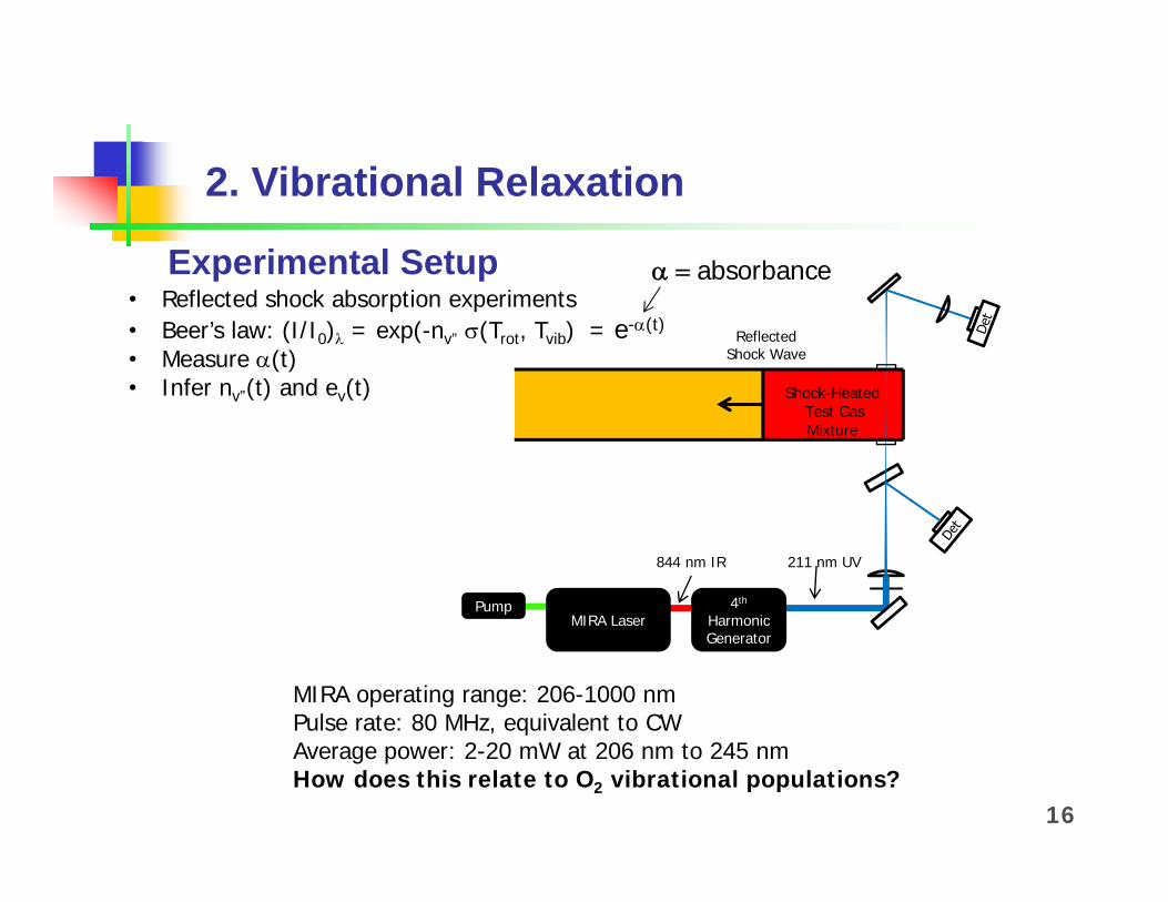
2. Vibrational Relaxation
16
ReflectedShock Wave
MIRA LaserPump 4th
Harmonic Generator
844 nm IR 211 nm UV
Shock-HeatedTest Gas Mixture
MIRA operating range: 206-1000 nmPulse rate: 80 MHz, equivalent to CWAverage power: 2-20 mW at 206 nm to 245 nmHow does this relate to O2 vibrational populations?
• Reflected shock absorption experiments• Beer’s law: (I/I0) = exp(-nv” (Trot, Tvib) = e-(t)
• Measure (t)• Infer nv”(t) and ev(t)
Experimental Setup absorbance
17
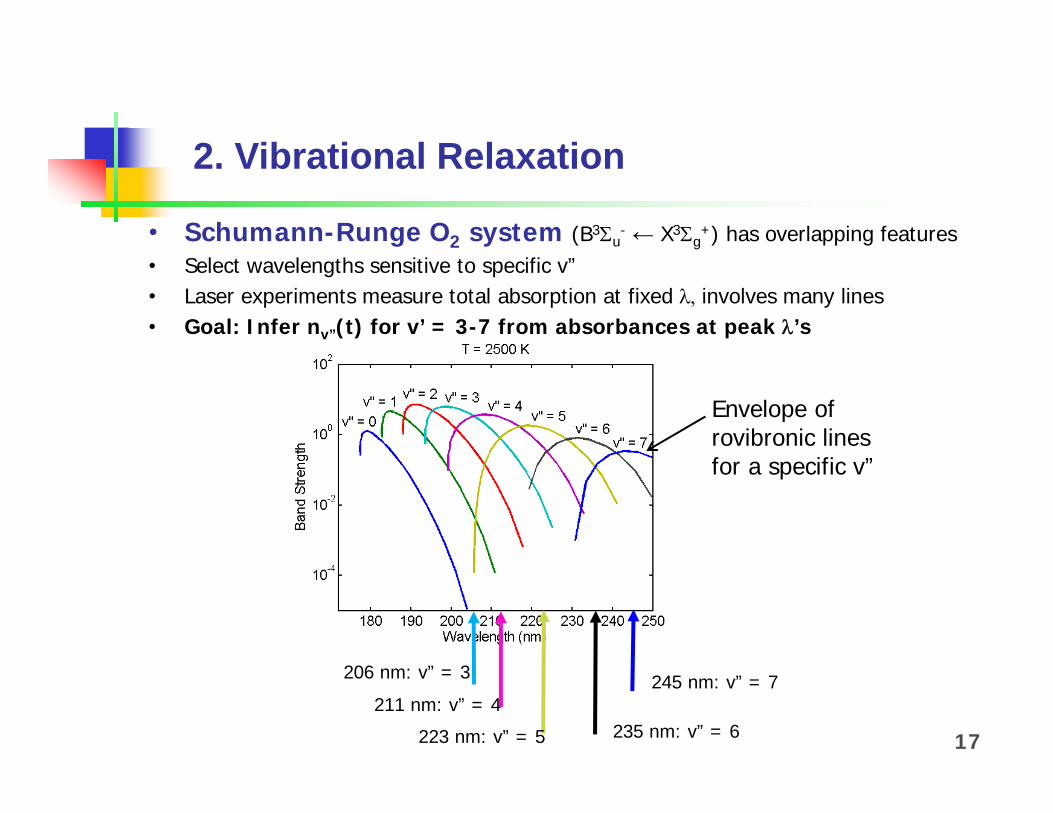
2. Vibrational Relaxation
• Schumann-Runge O2 system (B3u- ← X3g
+) has overlapping features • Select wavelengths sensitive to specific v”• Laser experiments measure total absorption at fixed involves many lines• Goal: Infer nv”(t) for v’ = 3-7 from absorbances at peak ’s
211 nm: v” = 4
223 nm: v” = 5
206 nm: v” = 3
Envelope of rovibronic lines for a specific v”
245 nm: v” = 7
235 nm: v” = 6

2. Example O2 Data and Model
18
• excellent signal-to-noise ratio (noise ~0.3% absorbance)• High-accuracy determination of XO2, T5, P5
• high-accuracy measurement of tvib!• Initial data support an evolving Boltzmann distribution for evib
• tvib can be plotted on a Landau-Teller plot

19
O2 vibrational relaxation measurements
• Current work inclose agreement with classic studies (Millikan and White (1963), but with much lower scatter
• Experiments with varying O2 fraction VT(O2-O2) and VT(O2-Ar)
1950K 1166K
Mixture Rule for (1/P)mix = Xj/Pj j
2. Landau-Teller Plot

3. Ignition Studies
1. Kinetics of branched chain reactions2. Definition of ignition3. Examples
20

21
3.1. Kinetics of Branched Chain Reactions:Basic Mechanism for Hydrogen Oxidation
by adsorb
2 2 2
2 2
2
2
2 2
1 + initiation
2 propagation
3 branching
4
5
6 8 , , wall removal
H O HO H
OH H H H O
H O OH O
O H OH H
H O M HO M
H O OH
tion, wall-catalyzed reactions stable species
termination
Build up of a radical pool during oxidation This characterizes ignition! Also exothermic reactions generate heat
release/pressure increase
2
2 2
2
2 2
2 2 2
Step 1:
Step 2:
Step 3:
Step 4:
net: 3 3 2 2 !
H O OH O
OH H H H O
O H OH H
OH H H H O
H O H H H O H
Net effect of branching is to create radicals
22
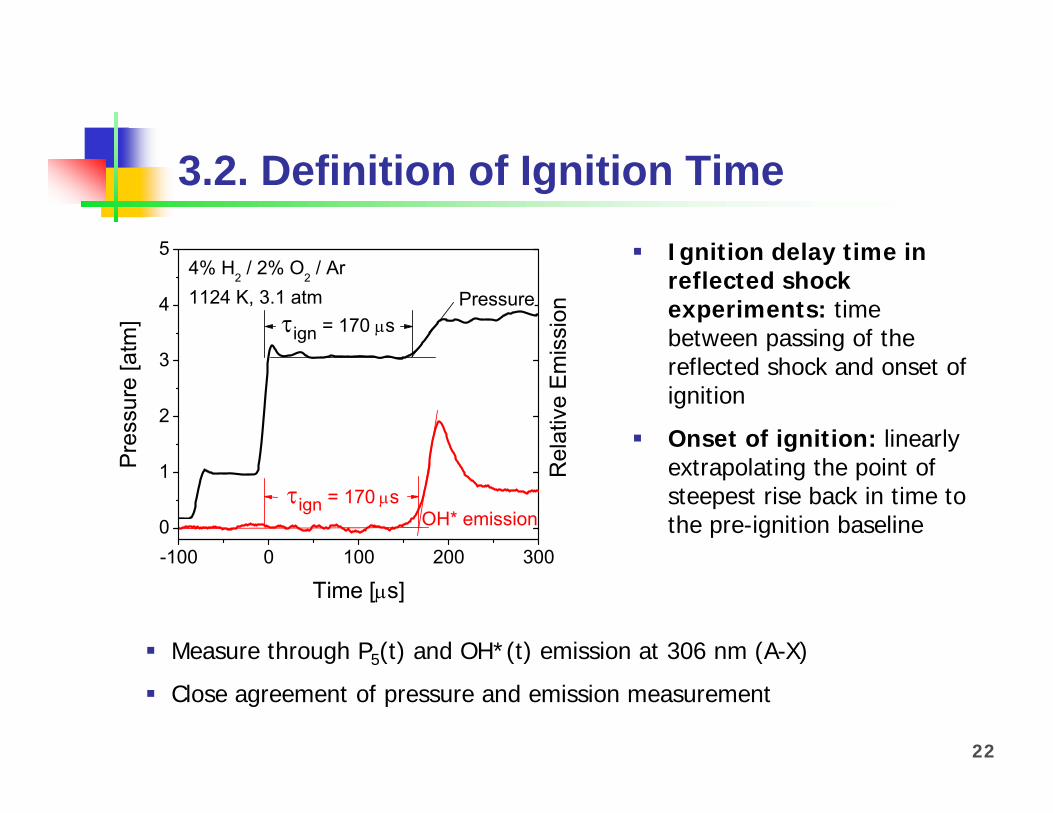
3.2. Definition of Ignition Time
Ignition delay time in reflected shock experiments: time between passing of the reflected shock and onset of ignition
Onset of ignition: linearly extrapolating the point of steepest rise back in time to the pre-ignition baseline
-100 0 100 200 3000
1
2
3
4
5
OH* emission
Rel
ativ
e E
mis
sion
Pre
ssur
e [a
tm]
Time [s]
ign = 170 s
4% H2 / 2% O2 / Ar1124 K, 3.1 atm Pressure
ign = 170s
Measure through P5(t) and OH*(t) emission at 306 nm (A-X)
Close agreement of pressure and emission measurement
23
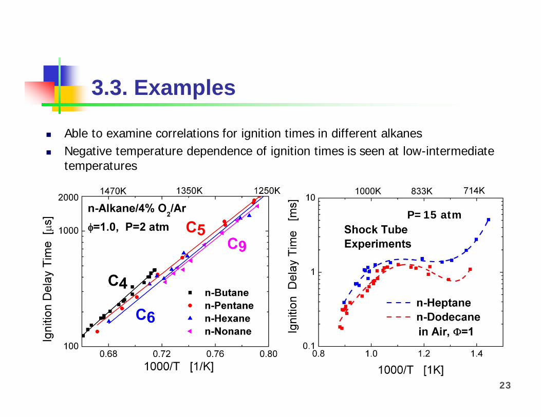
3.3. Examples
Able to examine correlations for ignition times in different alkanes Negative temperature dependence of ignition times is seen at low-intermediate
temperatures
P=15 atm
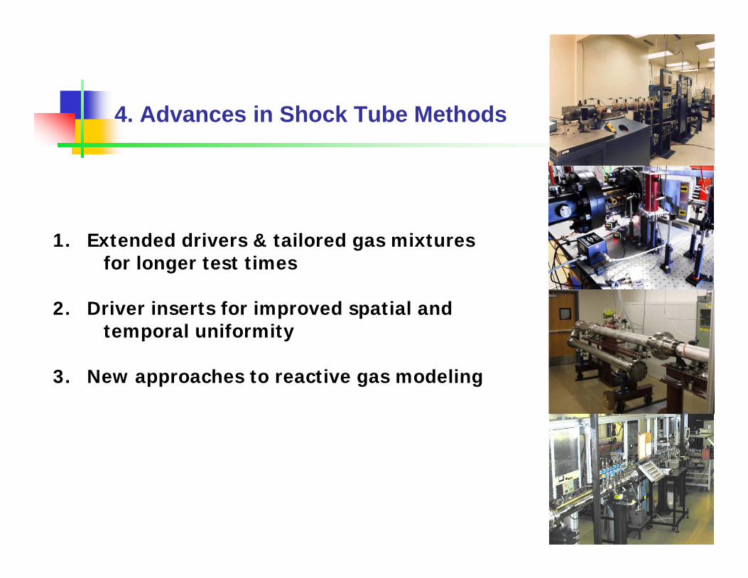
4. Advances in Shock Tube Methods
1. Extended drivers & tailored gas mixturesfor longer test times
2. Driver inserts for improved spatial andtemporal uniformity
3. New approaches to reactive gas modeling

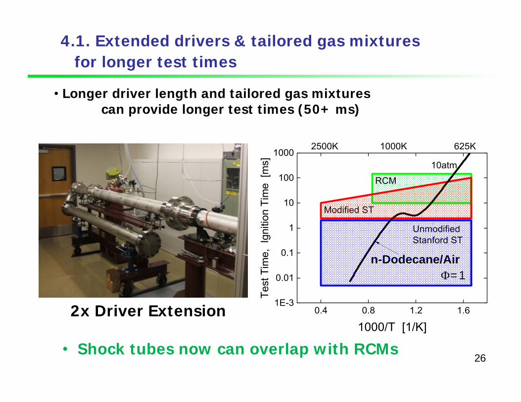
4.1. Extended drivers & tailored gas mixturesfor longer test times
• Conventional shock tube operation: ~ 1-3 ms test time• No overlap with RCM operation~ 10-150 ms test time
0.4 0.8 1.2 1.61E-3
0.01
0.1
1
10
100
1000
Test
Tim
e, I
gniti
on T
ime
[ms]
1000/T [1/K]
2500K 1000K 625K
UnmodifiedStanford ST
n-Dodecane/Air
10atm
0.4 0.8 1.2 1.61E-3
0.01
0.1
1
10
100
1000
Test
Tim
e, I
gniti
on T
ime
[ms]
1000/T [1/K]
2500K 1000K 625K
UnmodifiedStanford ST
RCM
n-Dodecane/Air
10atm
=1
25
0.4 0.8 1.2 1.61E-3
0.01
0.1
1
10
100
1000
Test
Tim
e, I
gniti
on T
ime
[ms]
1000/T [1/K]
2500K 1000K 625K
UnmodifiedStanford ST
Modified ST
RCM
n-Dodecane/Air
10atm
• Longer driver length and tailored gas mixturescan provide longer test times (50+ ms)
2x Driver Extension
• Shock tubes now can overlap with RCMs
=1
4.1. Extended drivers & tailored gas mixturesfor longer test times
26
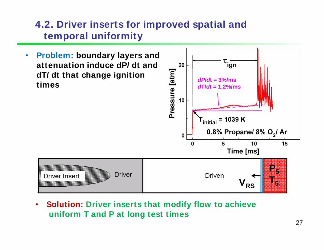
4.2. Driver inserts for improved spatial andtemporal uniformity
• Problem: boundary layers and attenuation induce dP/dt and dT/dt that change ignition times
dP/dt = 3%/msdT/dt = 1.2%/ms
• Solution: Driver inserts that modify flow to achieveuniform T and P at long test times
P5T5VRS
27
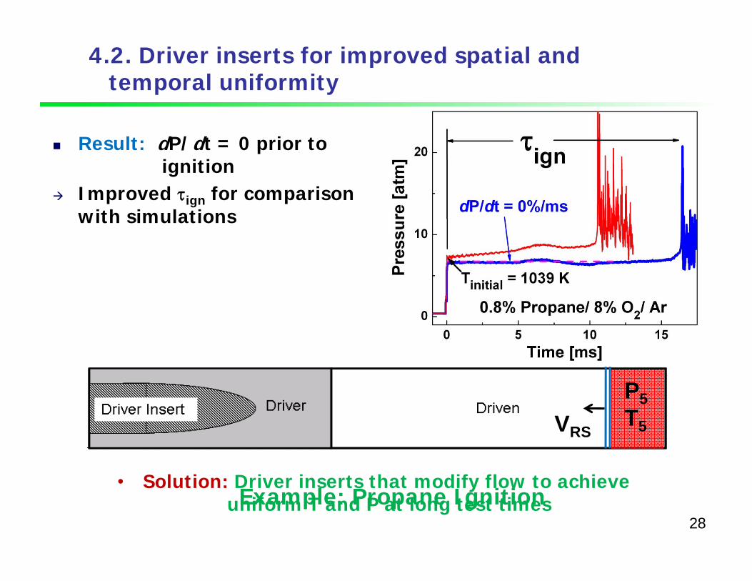
4.2. Driver inserts for improved spatial andtemporal uniformity
Result: dP/dt = 0 prior toignition
Improved ign for comparison with simulations
P5T5VRS
Example: Propane Ignition• Solution: Driver inserts that modify flow to achieve
uniform T and P at long test times28
4.2. Driver inserts for improved spatial andtemporal uniformity
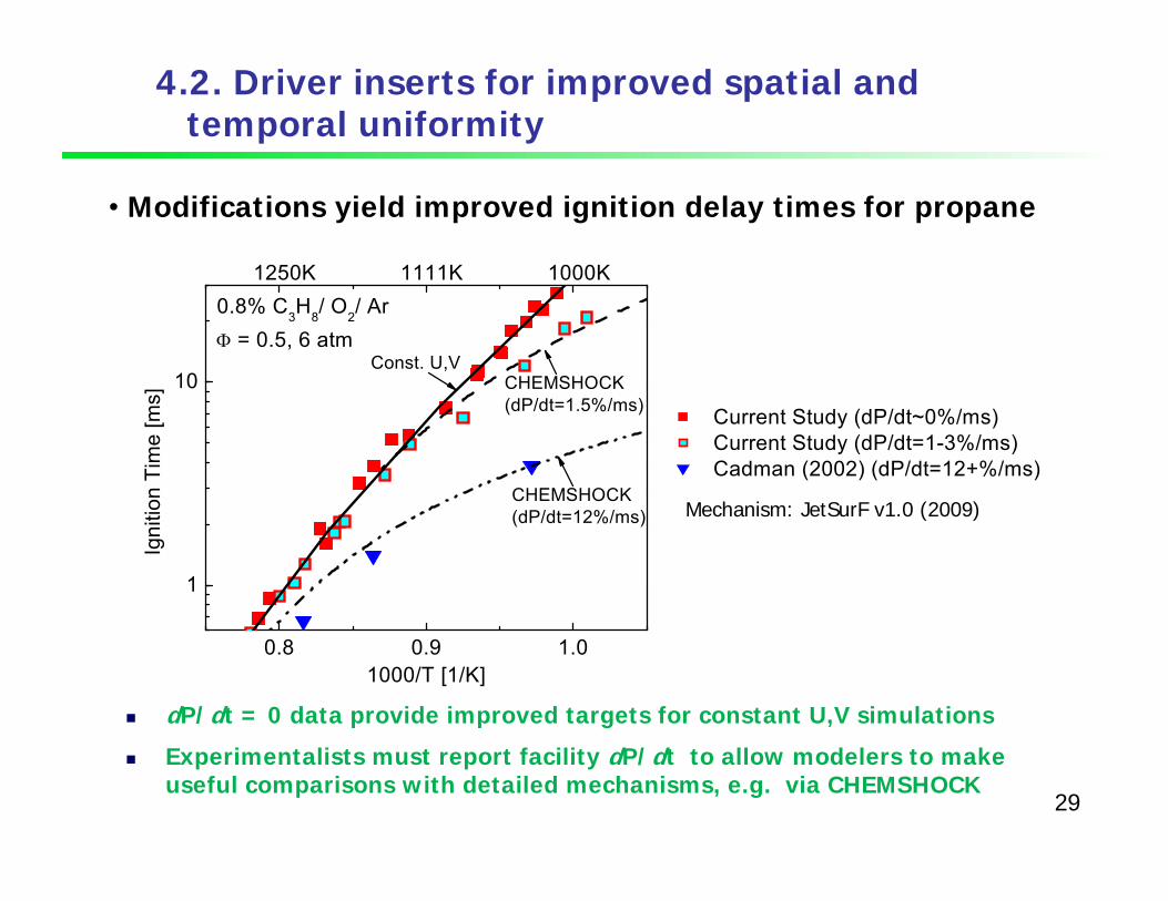
dP/dt = 0 data provide improved targets for constant U,V simulations
Experimentalists must report facility dP/dt to allow modelers to make useful comparisons with detailed mechanisms, e.g. via CHEMSHOCK
0.8 0.9 1.0
1
10
CHEMSHOCK(dP/dt=12%/ms)
CHEMSHOCK(dP/dt=1.5%/ms) Current Study (dP/dt~0%/ms)
Current Study (dP/dt=1-3%/ms) Cadman (2002) (dP/dt=12+%/ms)
1000K1111K1250K
Igni
tion
Tim
e [m
s]
1000/T [1/K]
0.8% C3H8/ O2/ Ar= 0.5, 6 atm
Const. U,V
Mechanism: JetSurF v1.0 (2009)
29
• Modifications yield improved ignition delay times for propane
4.3. New approaches to reactive gas modeling
Most current reflected shock modeling assumes Constant Volume or Constant Pressure
But: Reflected shock reactions are not Constant V or Constant P
processes!
Example: Heptane Ignition
30
Reactive Gasdynamics Modeling: The Problem

4.3. New approaches to reactive gas modeling
• This is not a Constant P process!
-100 0 100 200 300 400 500 6000
1
2
3
4
5
0.4% Heptane/4.4% O2/Ar, =11380K, 2.3 atm
Pre
ssur
e [a
tm]
Time [us]
ign
0
2
4
MeasuredSidewall P
Constant PModel
31
• Effect of Energy Release on P Profiles: n-Heptane Oxidation

4.3. New approaches to reactive gas modeling
• This is not a Constant P process!• Also not a Constant V process!• So how can entire process be modeled?
-100 0 100 200 300 400 500 6000
1
2
3
4
5
0.4% Heptane/4.4% O2/Ar, =11380K, 2.3 atm
Pre
ssur
e [a
tm]
Time [us]
ign
0
2
4
MeasuredSidewall P
Constant PModel
Constant V Model
32
• Effect of Energy Release on P Profiles: n-Heptane Oxidation
4.3. New approaches to reactive gas modeling
Minimize fuel loading to reduce exothermically- or endothermically-driven T and P changes- enabled by high-sensitivity laser diagnostics
Use new constrained reaction volume (CRV) concept to minimize pressure perturbations- enables constant P (or specified P) modeling
33
• Proposed Solutions to Enable Modeling through Entire Combustion Event
4.3. New approaches to reactive gas modeling
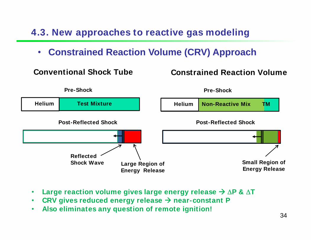
• Large reaction volume gives large energy release P & T• CRV gives reduced energy release near-constant P• Also eliminates any question of remote ignition!
Conventional Shock Tube Constrained Reaction Volume
Helium Test Mixture
Pre-Shock
Post-Incident Shock
Pre-Shock
Post-Incident Shock
Helium Non-Reactive Mix TM
Large Region ofEnergy Release
Small Region ofEnergy Release
ReflectedShock Wave
Post-Reflected Shock Post-Reflected Shock
34
• Constrained Reaction Volume (CRV) Approach
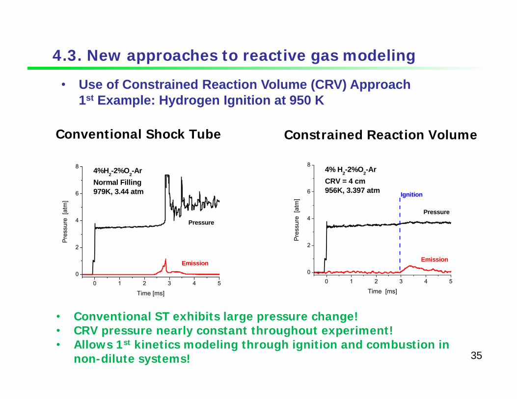
• Conventional ST exhibits large pressure change!• CRV pressure nearly constant throughout experiment!• Allows 1st kinetics modeling through ignition and combustion in
non-dilute systems!
Conventional Shock Tube Constrained Reaction Volume
0 1 2 3 4 50
2
4
6
8
Pressure
4%H2-2%O2-ArNormal Filling979K, 3.44 atm
Pres
sure
[at
m]
Time [ms]
Emission
0 1 2 3 4 50
2
4
6
8
Pressure
4% H2-2%O2-ArCRV = 4 cm956K, 3.397 atm
Pre
ssur
e [a
tm]
Time [ms]
Emission
Ignition
4.3. New approaches to reactive gas modeling
35
• Use of Constrained Reaction Volume (CRV) Approach1st Example: Hydrogen Ignition at 950 K
4.3. New approaches to reactive gas modeling
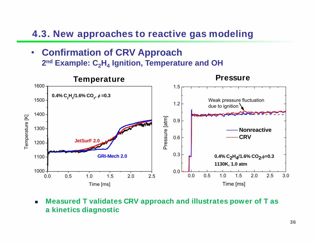
Measured T validates CRV approach and illustrates power of T as a kinetics diagnostic
36
Temperature Pressure
0.0 0.5 1.0 1.5 2.0 2.51000
1100
1200
1300
1400
1500
1600
JetSurF 2.0
0.4% C2H4/1.6% CO2, =0.3
Time [ms]
Tem
pera
ture
[K]
GRI-Mech 2.0
0.0 0.5 1.0 1.5 2.0 2.5 3.00.0
0.3
0.6
0.9
1.2
1.5
Nonreactive CRV
Time [ms]
Pre
ssur
e [a
tm]
Weak pressure fluctuation due to ignition
0.4% C2H4/1.6% CO2,=0.31130K, 1.0 atm
• Confirmation of CRV Approach2nd Example: C2H4 Ignition, Temperature and OH
• CRV & conventional filling data agree at at high T
• CRV yields longer delay times at lower T than conventional filling
• CRV provides true constant H, P data, conventional data are difficult to model
4.3. New approaches to reactive gas modeling
0.8 1.0 1.2 1.40.1
1
10 CRV Strategy Conventional Filling
1-butanol/air20 atm, = 1.0
All data scaled by P-1
714K833K1000K1250K
1000/T (1/K)
t ign (
ms)
37
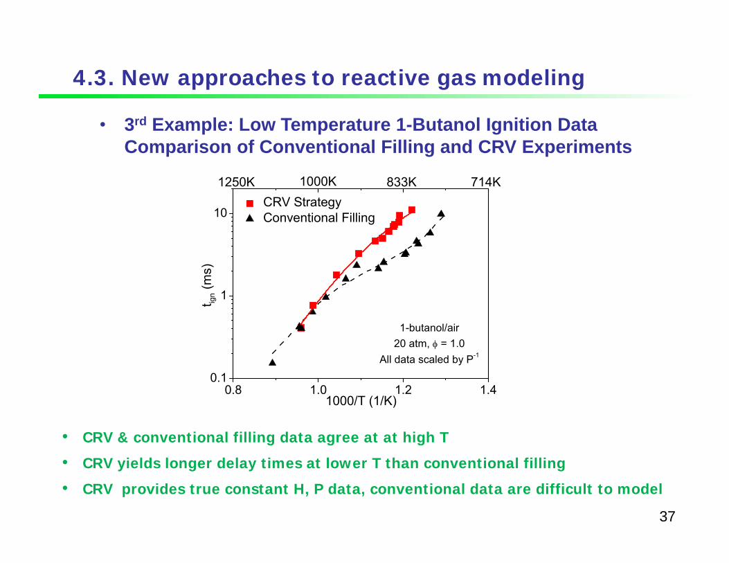
• 3rd Example: Low Temperature 1-Butanol Ignition DataComparison of Conventional Filling and CRV Experiments

• CRV & conventional filling data agree at at high T
• CRV yields longer delay times at lower T than conventional filling
• CRV provides true constant H, P data, conventional data are difficult to model
4.3. New approaches to reactive gas modeling
38
• 3rd Example: Low Temperature 1-Butanol Ignition DataComparison of Conventional Filling and CRV Experiments
0.8 1.0 1.2 1.40.1
1
10 CRV Strategy Conventional Filling
1-butanol/air20 atm, = 1.0
714K833K1000K1250K
1000/T (1/K)
t ign (
ms)
Solid Line:Sarathy et al. (2012)
Current models are in agreement with CRV constant P data!
Next: Shock Tube Applications with Lasers
Elementary Reactions Multi-Species Time-Histories