Lecture 11 Results and Post Processing - Rice University © 2015 ANSYS, Inc. February 27, 2015 16.0...

1 © 2015 ANSYS, Inc. February 27, 2015

16.0 Release

Lecture 11 Results and Post Processing

Introduction to ANSYS Mechanical


Chapter Overview In this chapter controlling the display of results and the detection of potential results errors due to poor mesh quality will be covered:

A. Demonstration

B. Section Planes

C. Probe Tool

D. Charts

E. Scoping Results

F. Coordinate systems

G. Linearized Stress

H. Error Estimation

I. Convergence

J. Stress Singularities

K. Convergence and Scoping

L. Workshop 11.1 – Results Processing

M.Appendix


Chapter Overview In this chapter controlling the display of results and the detection of potential results errors due to poor mesh quality will be covered:

A Demonstration video showing post processing tools is available with this training material.

The Lecture covers features which do not appear in the video.


A. Demonstration

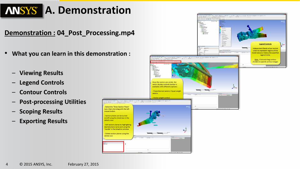
Demonstration : 04_Post_Processing.mp4

• What you can learn in this demonstration :

– Viewing Results

– Legend Controls

– Contour Controls

– Post-processing Utilities

– Scoping Results

– Exporting Results


B. Section planes

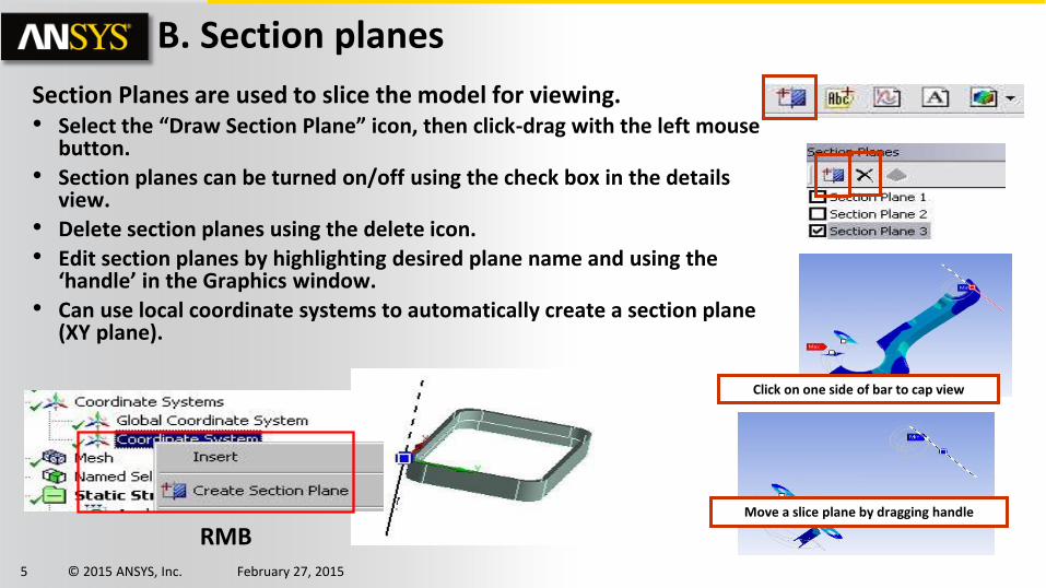
Section Planes are used to slice the model for viewing. • Select the “Draw Section Plane” icon, then click-drag with the left mouse

button.

• Section planes can be turned on/off using the check box in the details view.

• Delete section planes using the delete icon.

• Edit section planes by highlighting desired plane name and using the ‘handle’ in the Graphics window.

• Can use local coordinate systems to automatically create a section plane (XY plane).

Move a slice plane by dragging handle

Click on one side of bar to cap view

RMB


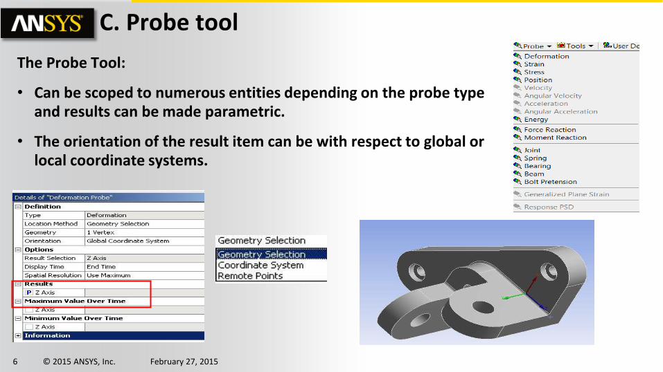
C. Probe tool

The Probe Tool:

• Can be scoped to numerous entities depending on the probe type and results can be made parametric.

• The orientation of the result item can be with respect to global or local coordinate systems.


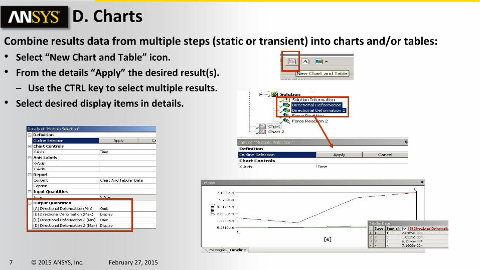
D. Charts Combine results data from multiple steps (static or transient) into charts and/or tables:

• Select “New Chart and Table” icon.

• From the details “Apply” the desired result(s).

– Use the CTRL key to select multiple results.

• Select desired display items in details.


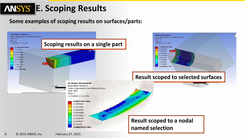
E. Scoping Results Some examples of scoping results on surfaces/parts:

Scoping results on a single part

Result scoped to selected surfaces

Result scoped to a nodal named selection


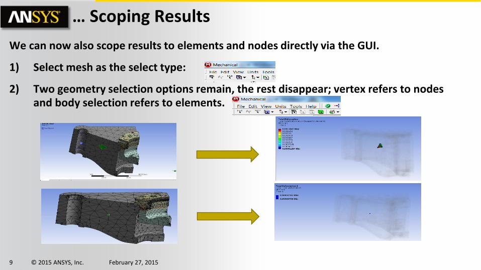
We can now also scope results to elements and nodes directly via the GUI.

1) Select mesh as the select type:

2) Two geometry selection options remain, the rest disappear; vertex refers to nodes and body selection refers to elements.

… Scoping Results


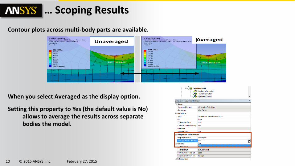
… Scoping Results

Contour plots across multi-body parts are available.

When you select Averaged as the display option.

Setting this property to Yes (the default value is No) allows to average the results across separate bodies the model.


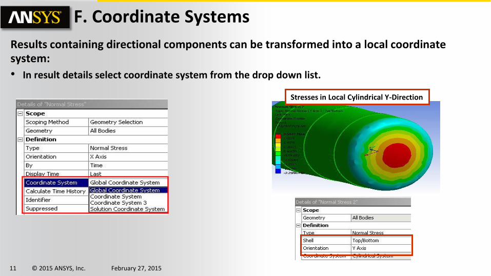
F. Coordinate Systems

Results containing directional components can be transformed into a local coordinate system:

• In result details select coordinate system from the drop down list.

Stresses in Local Cylindrical Y-Direction


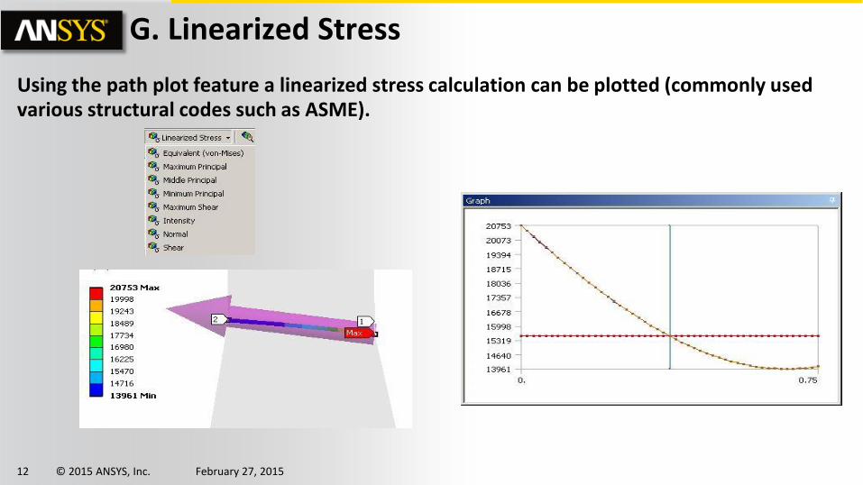
G. Linearized Stress

Using the path plot feature a linearized stress calculation can be plotted (commonly used various structural codes such as ASME).


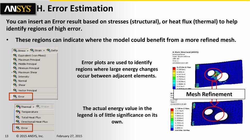
H. Error Estimation You can insert an Error result based on stresses (structural), or heat flux (thermal) to help identify regions of high error.

• These regions can indicate where the model could benefit from a more refined mesh.

Error plots are used to identify regions where large energy changes occur between adjacent elements.

The actual energy value in the legend is of little significance on its

own.

Mesh Refinement


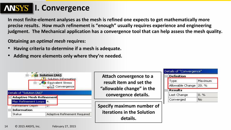
I. Convergence In most finite-element analyses as the mesh is refined one expects to get mathematically more precise results. How much refinement is “enough” usually requires experience and engineering judgment. The Mechanical application has a convergence tool that can help assess the mesh quality.

Obtaining an optimal mesh requires:

• Having criteria to determine if a mesh is adequate.

• Adding more elements only where they’re needed.

Attach convergence to a result item and set the

“allowable change” in the convergence details.

Specify maximum number of iterations in the Solution

details.


… Convergence

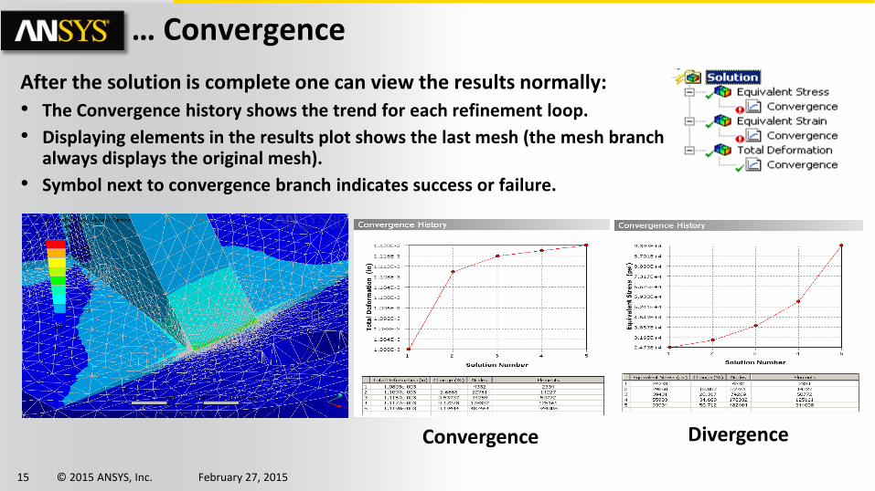
After the solution is complete one can view the results normally:

• The Convergence history shows the trend for each refinement loop.

• Displaying elements in the results plot shows the last mesh (the mesh branch always displays the original mesh).

• Symbol next to convergence branch indicates success or failure.

Convergence Divergence


… Convergence

Convergence tool cannot be used if:

• The model contains mesh connection object

• You have an upstream or a downstream analysis link

• You import loads in the analysis

To use Convergence, you must set ”Calculate Stress” to ”Yes” under Output Controls in the Analysis Settings details panel.


J. Stress Singularities

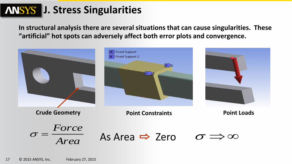
In structural analysis there are several situations that can cause singularities. These “artificial” hot spots can adversely affect both error plots and convergence.

Crude Geometry Point Constraints Point Loads

Area

Force As Area Zero


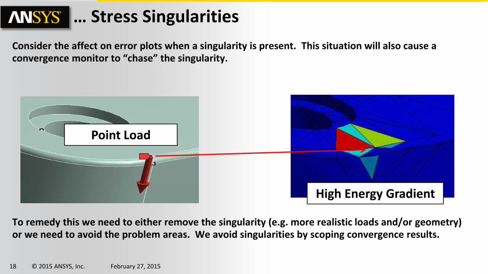
… Stress Singularities

Consider the affect on error plots when a singularity is present. This situation will also cause a convergence monitor to “chase” the singularity.

To remedy this we need to either remove the singularity (e.g. more realistic loads and/or geometry) or we need to avoid the problem areas. We avoid singularities by scoping convergence results.

Point Load

High Energy Gradient


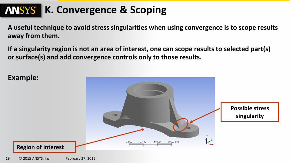
K. Convergence & Scoping

A useful technique to avoid stress singularities when using convergence is to scope results away from them.

If a singularity region is not an area of interest, one can scope results to selected part(s) or surface(s) and add convergence controls only to those results.

Example:

Possible stress singularity

Region of interest


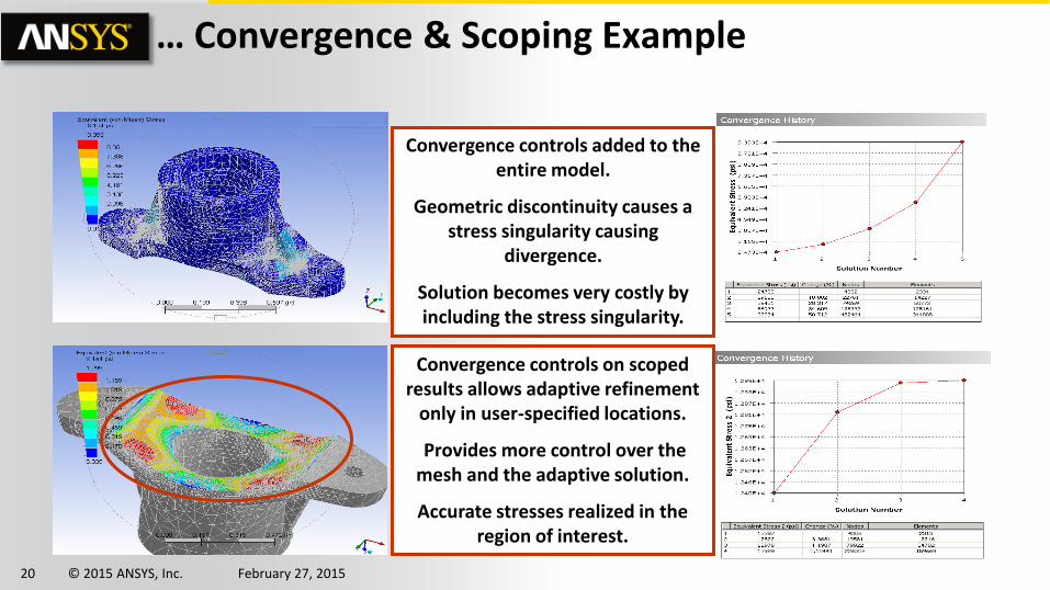
… Convergence & Scoping Example

Convergence controls added to the entire model.

Geometric discontinuity causes a stress singularity causing

divergence.

Solution becomes very costly by including the stress singularity.

Convergence controls on scoped results allows adaptive refinement

only in user-specified locations.

Provides more control over the mesh and the adaptive solution.

Accurate stresses realized in the region of interest.


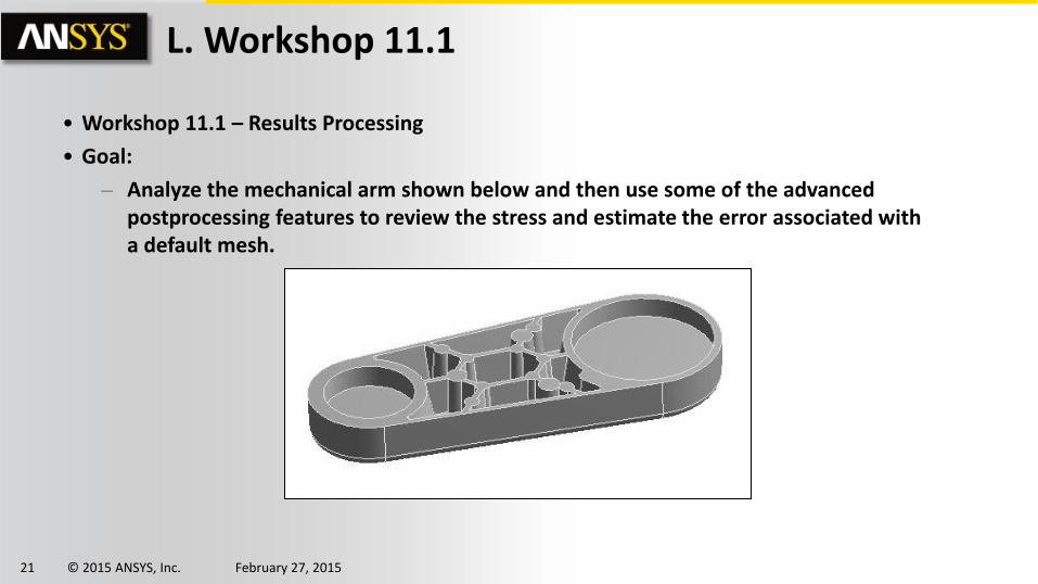
• Workshop 11.1 – Results Processing

• Goal:

– Analyze the mechanical arm shown below and then use some of the advanced postprocessing features to review the stress and estimate the error associated with a default mesh.

L. Workshop 11.1


M. Appendix

• Viewing Results • Legend Controls • Contour Controls • Alert • Windows • Videos • CE display • Scoping Results • Exporting Results


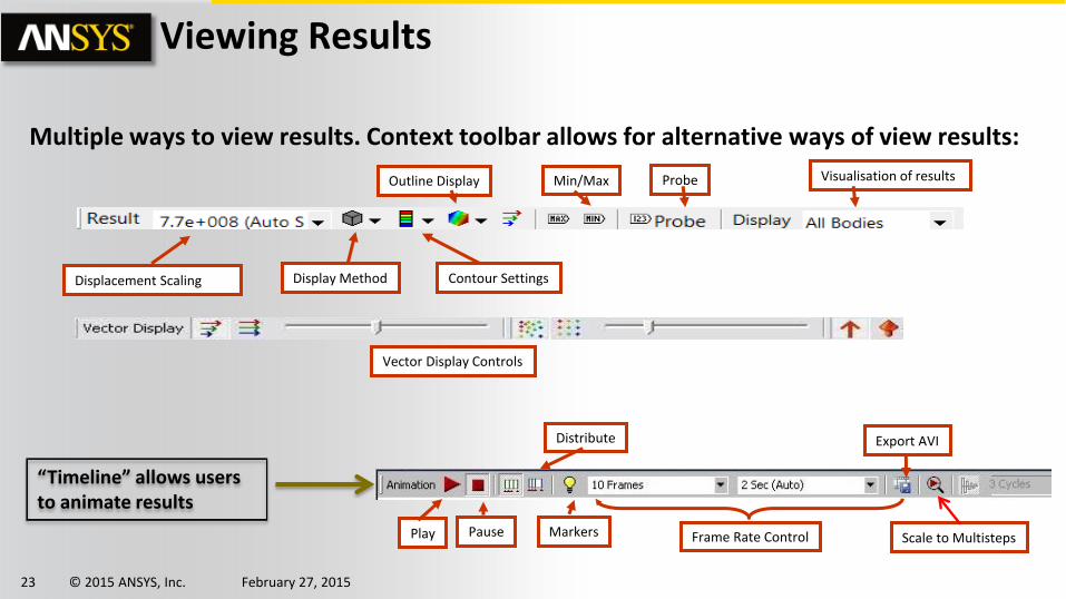
Viewing Results

Multiple ways to view results. Context toolbar allows for alternative ways of view results:

Vector Display Controls

Min/Max

Displacement Scaling Display Method Contour Settings

Outline Display Probe

Play Pause

Distribute

Markers Frame Rate Control

Export AVI

Scale to Multisteps

“Timeline” allows users to animate results

Visualisation of results


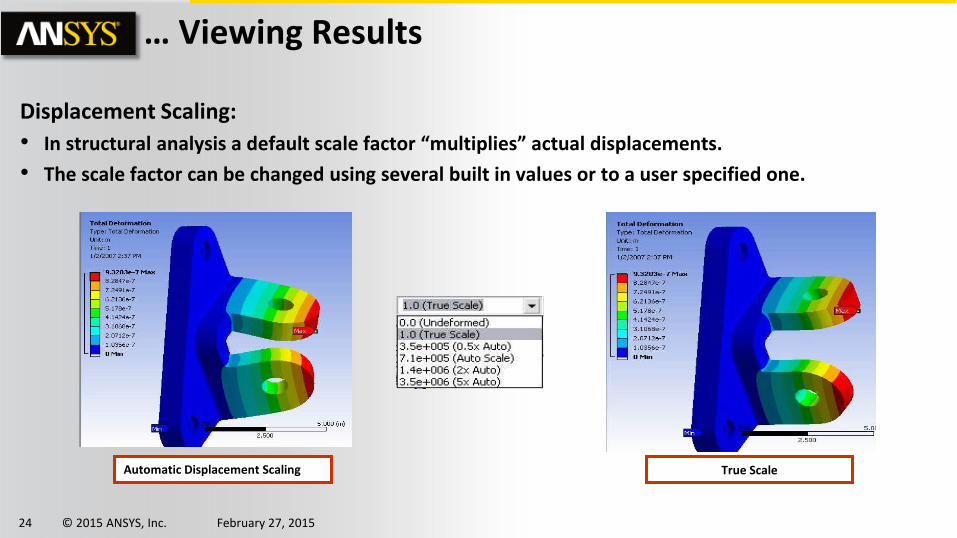
… Viewing Results

Displacement Scaling:

• In structural analysis a default scale factor “multiplies” actual displacements.

• The scale factor can be changed using several built in values or to a user specified one.

True Scale Automatic Displacement Scaling


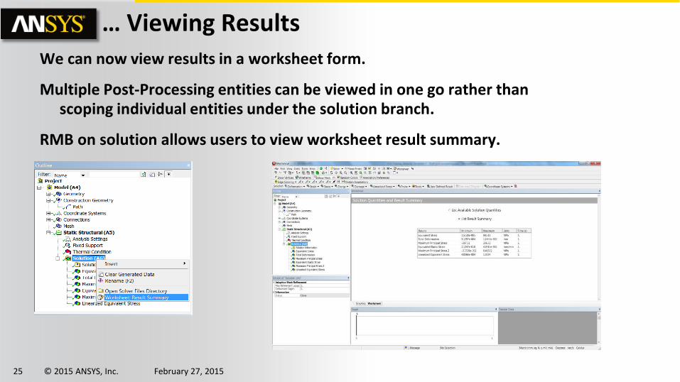
… Viewing Results We can now view results in a worksheet form.

Multiple Post-Processing entities can be viewed in one go rather than scoping individual entities under the solution branch.

RMB on solution allows users to view worksheet result summary.


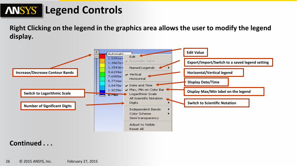
Right Clicking on the legend in the graphics area allows the user to modify the legend display.

Continued . . .

Legend Controls

Edit Value

Export/Import/Switch to a saved legend setting

Horizontal/Vertical legend

Display Date/Time

Display Max/Min label on the legend Switch to Logarithmic Scale

Switch to Scientific Notation Number of Significant Digits

Increase/Decrease Contour Bands


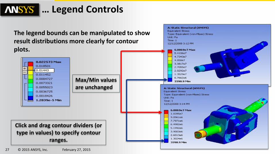
… Legend Controls

The legend bounds can be manipulated to show result distributions more clearly for contour plots.

Click and drag contour dividers (or type in values) to specify contour

ranges.

Max/Min values are unchanged


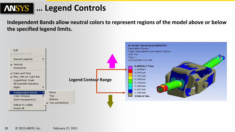
… Legend Controls

Independent Bands allow neutral colors to represent regions of the model above or below the specified legend limits.

Legend Contour Range


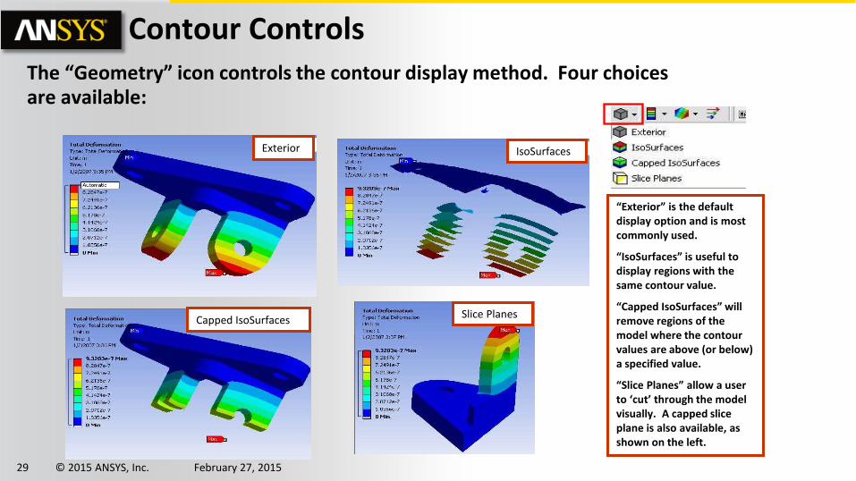
Contour Controls The “Geometry” icon controls the contour display method. Four choices are available:

“Exterior” is the default display option and is most commonly used.

“IsoSurfaces” is useful to display regions with the same contour value.

“Capped IsoSurfaces” will remove regions of the model where the contour values are above (or below) a specified value.

“Slice Planes” allow a user to ‘cut’ through the model visually. A capped slice plane is also available, as shown on the left.

Slice Planes

IsoSurfaces Exterior

Capped IsoSurfaces


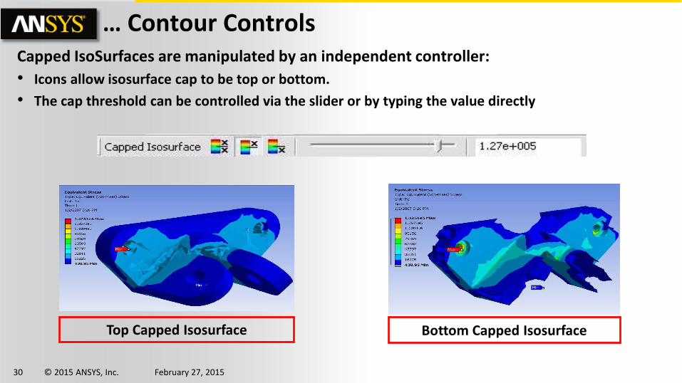
… Contour Controls Capped IsoSurfaces are manipulated by an independent controller:

• Icons allow isosurface cap to be top or bottom.

• The cap threshold can be controlled via the slider or by typing the value directly

Top Capped Isosurface Bottom Capped Isosurface


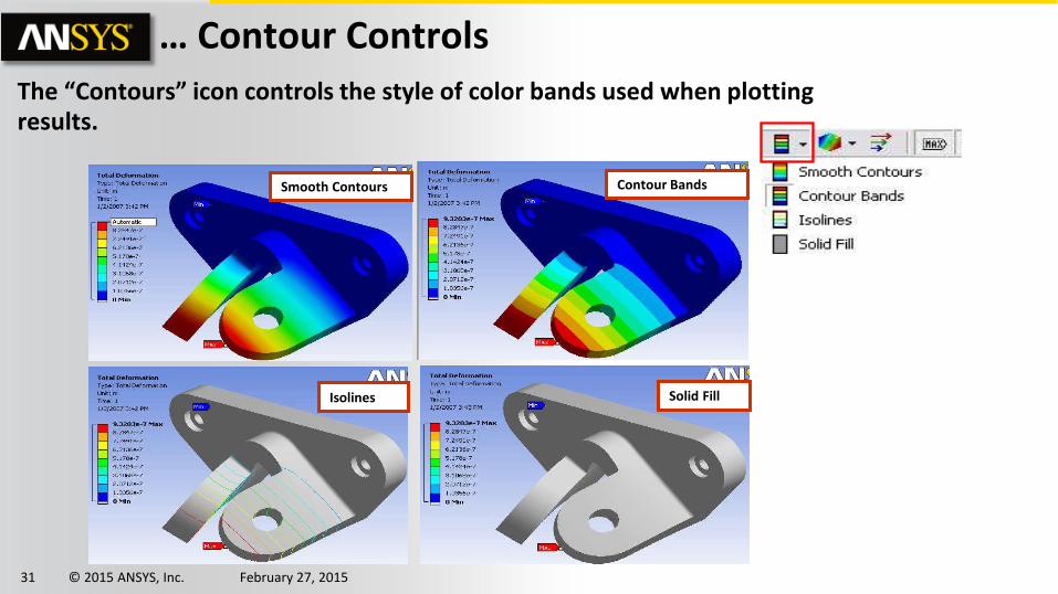
… Contour Controls The “Contours” icon controls the style of color bands used when plotting results.

Solid Fill

Contour Bands Smooth Contours

Isolines


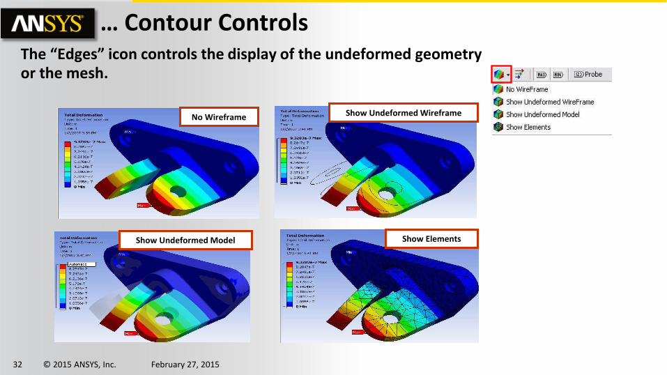
… Contour Controls The “Edges” icon controls the display of the undeformed geometry or the mesh.

No Wireframe Show Undeformed Wireframe

Show Undeformed Model Show Elements


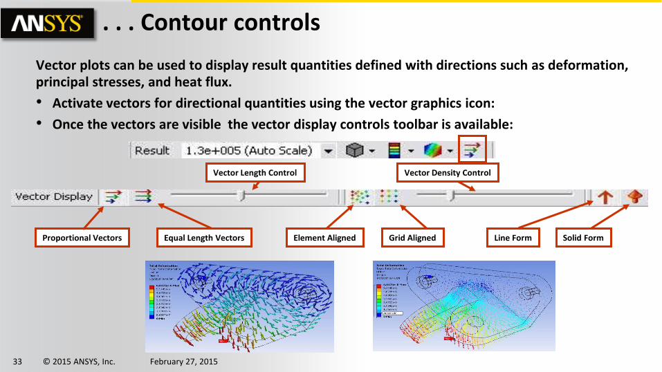
. . . Contour controls

Vector plots can be used to display result quantities defined with directions such as deformation, principal stresses, and heat flux.

• Activate vectors for directional quantities using the vector graphics icon:

• Once the vectors are visible the vector display controls toolbar is available:

Proportional Vectors Equal Length Vectors

Vector Length Control

Grid Aligned Element Aligned Line Form Solid Form

Vector Density Control

Equal Length Vectors

Vector Length Control

Grid Aligned Element Aligned Line Form Solid Form

Vector Density Control


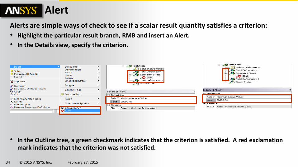
Alert Alerts are simple ways of check to see if a scalar result quantity satisfies a criterion:

• Highlight the particular result branch, RMB and insert an Alert.

• In the Details view, specify the criterion.

• In the Outline tree, a green checkmark indicates that the criterion is satisfied. A red exclamation mark indicates that the criterion was not satisfied.


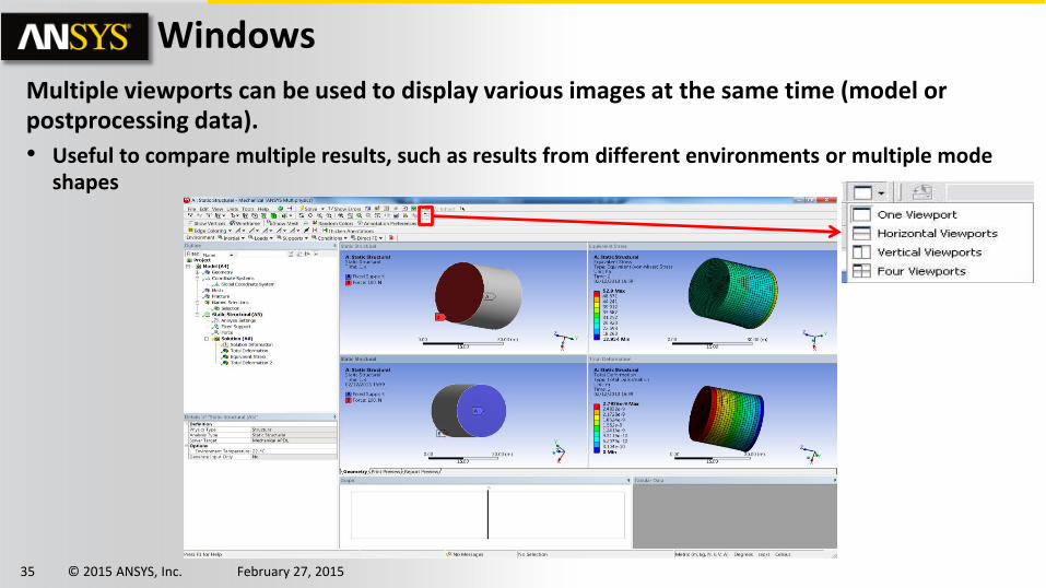
Windows Multiple viewports can be used to display various images at the same time (model or postprocessing data).

• Useful to compare multiple results, such as results from different environments or multiple mode shapes


Videos

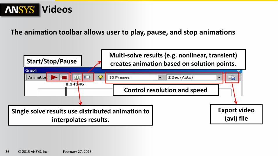
The animation toolbar allows user to play, pause, and stop animations

Start/Stop/Pause

Single solve results use distributed animation to interpolates results.

Export video (avi) file

Multi-solve results (e.g. nonlinear, transient) creates animation based on solution points.

Control resolution and speed


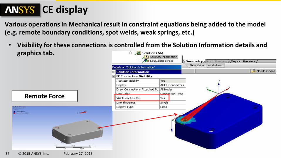
CE display Various operations in Mechanical result in constraint equations being added to the model (e.g. remote boundary conditions, spot welds, weak springs, etc.)

• Visibility for these connections is controlled from the Solution Information details and graphics tab.

Remote Force


Scoping Results

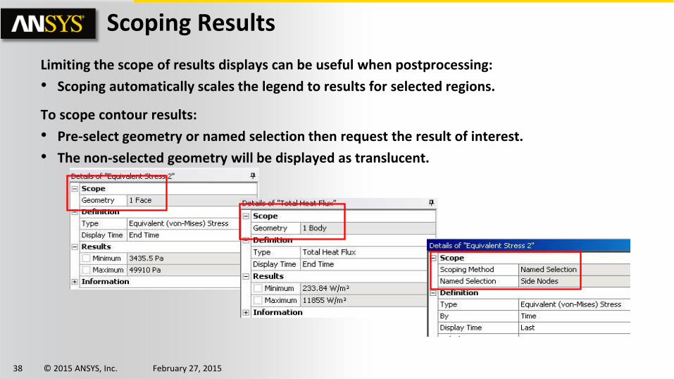
Limiting the scope of results displays can be useful when postprocessing:

• Scoping automatically scales the legend to results for selected regions.

To scope contour results:

• Pre-select geometry or named selection then request the result of interest.

• The non-selected geometry will be displayed as translucent.


… Scoping Results

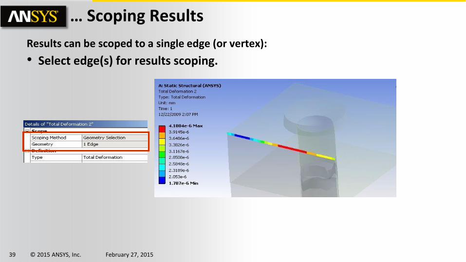
Results can be scoped to a single edge (or vertex):

• Select edge(s) for results scoping.


… Scoping Results

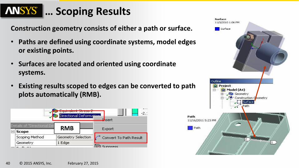
Construction geometry consists of either a path or surface.

• Paths are defined using coordinate systems, model edges or existing points.

• Surfaces are located and oriented using coordinate systems.

• Existing results scoped to edges can be converted to path plots automatically (RMB).

RMB


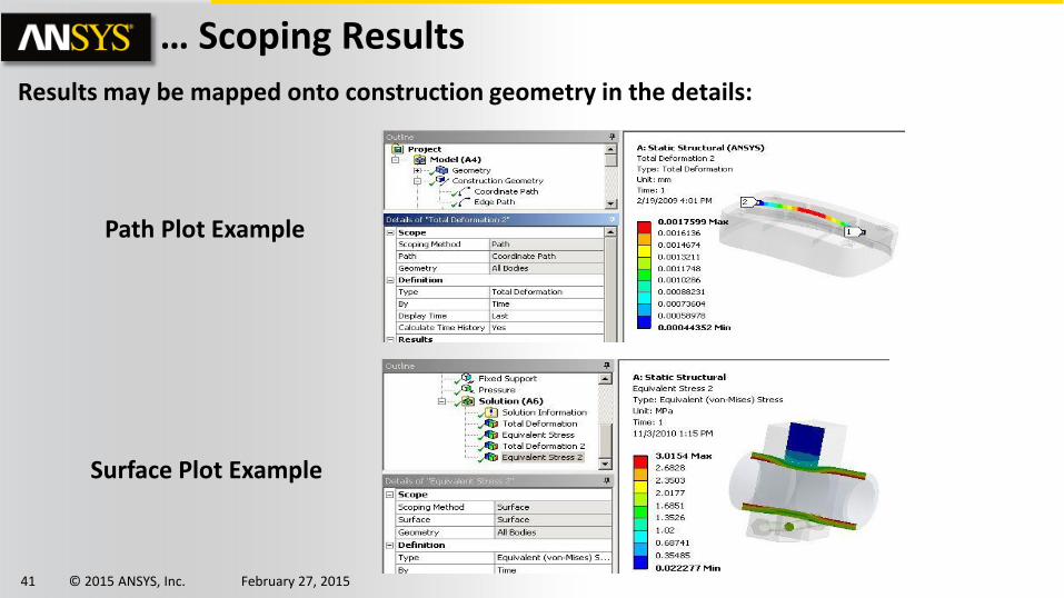
… Scoping Results Results may be mapped onto construction geometry in the details:

Path Plot Example

Surface Plot Example


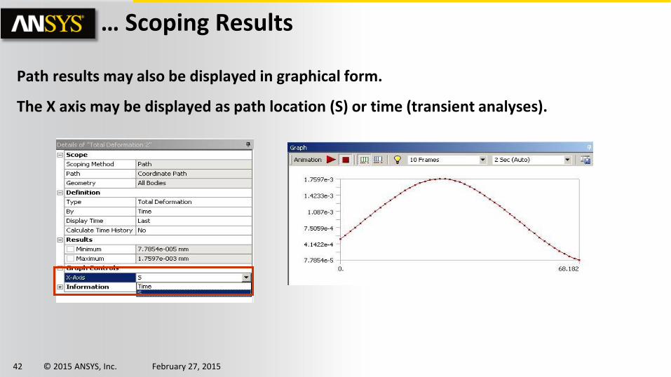
… Scoping Results

Path results may also be displayed in graphical form.

The X axis may be displayed as path location (S) or time (transient analyses).


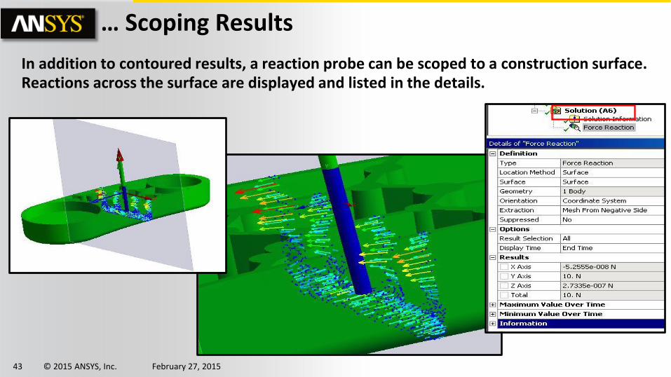
… Scoping Results

In addition to contoured results, a reaction probe can be scoped to a construction surface. Reactions across the surface are displayed and listed in the details.


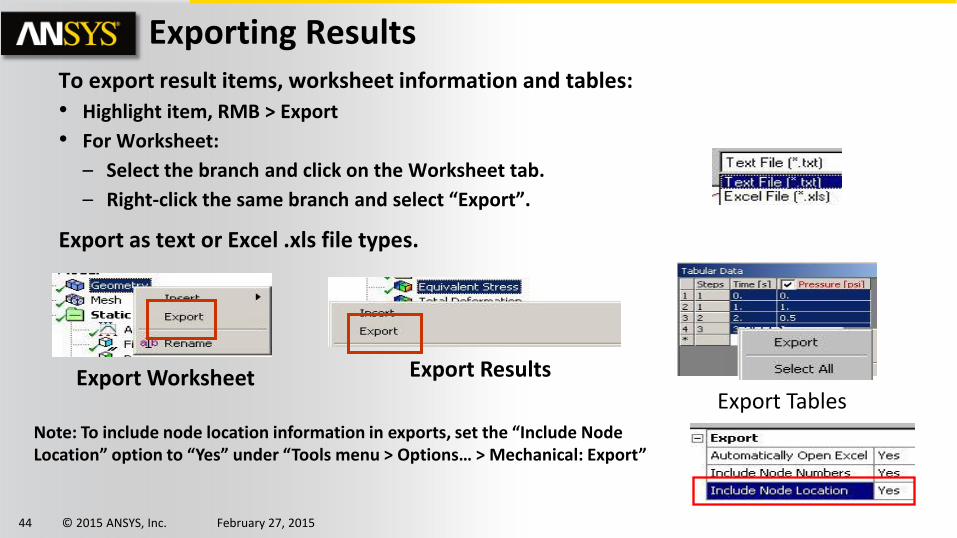
Exporting Results To export result items, worksheet information and tables:

• Highlight item, RMB > Export

• For Worksheet:

– Select the branch and click on the Worksheet tab.

– Right-click the same branch and select “Export”.

Export as text or Excel .xls file types.

Export Worksheet Export Results

Export Tables Note: To include node location information in exports, set the “Include Node Location” option to “Yes” under “Tools menu > Options… > Mechanical: Export”

Lecture 11 Results and Post Processing - Rice University © 2015 ANSYS, Inc. February 27, 2015 16.0...

Documents

Transcript of Lecture 11 Results and Post Processing - Rice University © 2015 ANSYS, Inc. February 27, 2015 16.0...