Fin 501:Asset Pricing I

Slide 11-1

Lecture 11: Multi-period

Equilibrium Models

Prof. Markus K. Brunnermeier

Fin 501:Asset Pricing I

Slide 11-2

Time-varying R*t (SDF)

• If one-period SDF mt is not time-varying (i.e.

distribution of mt is i.i.d., then

Expectations hypothesis holds

Investment opportunity set does not vary

Corresponding R* of single factor state-price beta

model can be easily estimate (because over time one

more and more observations about R*)

• If not, then mt (or corresponding R*t)

depends on state variable

multiple factor model

Fin 501:Asset Pricing I

Slide 11-3

R* depends on state variable

• R*t=R*(zt), with state variable zt

• Example:

zt = 1 or 2 with equal probability

Idea:

• Take all periods with zt=1 and figure out R*(1)

• Take all periods with zt=2 and figure out R*(2)

Can one do that?

• No – hedge across state variables

• Potential state-variables: predict future return

Fin 501:Asset Pricing I

Slide 11-4

Intertemporal CAPM (ICAPM)

• Merton (1973)

Fin 501:Asset Pricing I

Slide 11-5

Deriving ICAPM

• ICAPM allows consumption to depend on state

variable zt, which predicts future returns,

e.g. price-dividend ratio, risk-free rate

• Hence, value function V depends on both wealth

Wt and on state variable z

• Bellman equation

E[P1

t=0 ±tu(ct; zt)]

V (Wt; zt) = supct;Wtfu(ct; zt) + ±Et[V (Wt+1; zt+1]g

Fin 501:Asset Pricing I

Slide 11-6

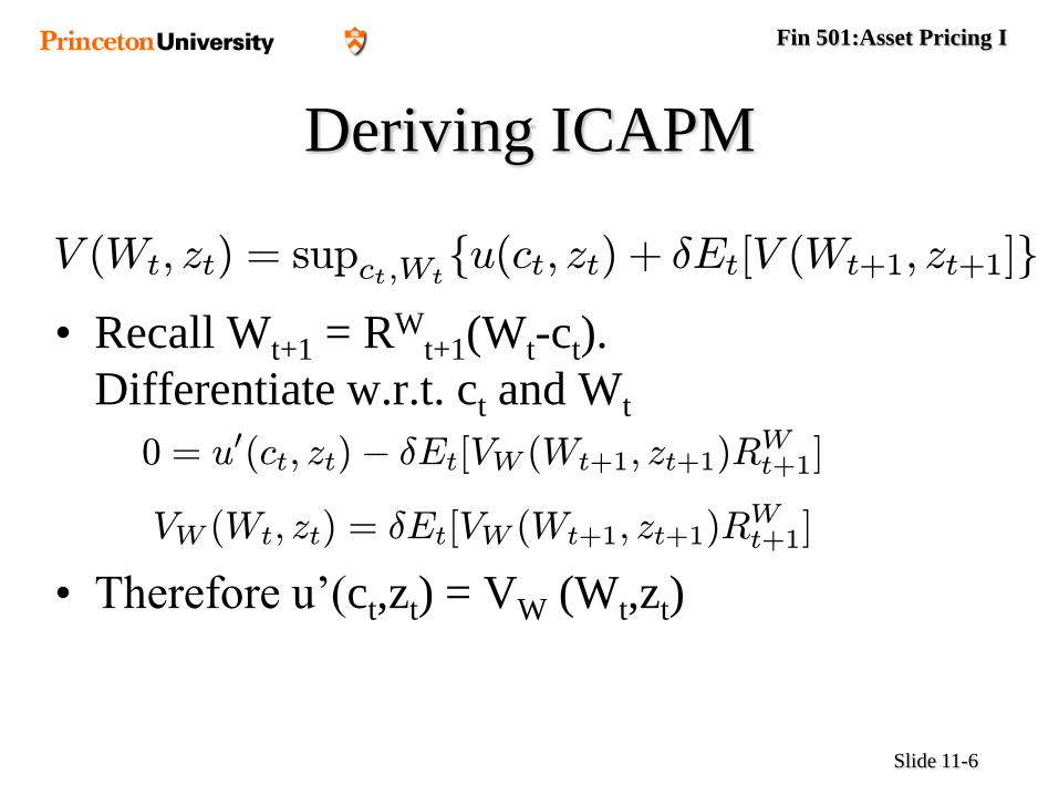
Deriving ICAPM

• Recall Wt+1 = RWt+1(Wt-ct).

Differentiate w.r.t. ct and Wt

• Therefore u’(ct,zt) = VW (Wt,zt)

V (Wt; zt) = supct;Wtfu(ct; zt) + ±Et[V (Wt+1; zt+1]g

0 = u0(ct; zt)¡ ±Et[VW (Wt+1; zt+1)RWt+1]

VW (Wt; zt) = ±Et[VW (Wt+1; zt+1)RWt+1]

Fin 501:Asset Pricing I

Slide 11-7

Deriving ICAPM

• Hence equation

becomes

• Using a first order approximation

we obtain

Where ° is relative risk aversion coefficient of V

Second term are additional “risk factors”

E[Rit+1]¡Rf =¡Covt(u

0(ct+1);Rit+1)

Et[u0(ct+1]

E[Rit+1]¡Rf =¡Covt(VW (Wt+1;zt+1);R

it+1)

Et[VW (Wt+1;zt+1)]

VW(Wt+1; zt+1) ¼ VW(Wt; zt) +VWW(Wt; zt)¢Wt+1 +VWz(Wt; zt)¢zt+1

E[Rit+1]¡Rf = ¡°Covt(¢Wt+1; R

it+1) +

VWz

Et[VW ]Cov(¢zt+1; R

it+1)

Fin 501:Asset Pricing I

Slide 11-8

Static problem = intertemporal problem

• In general ICAPM setting

CRRA with γ≠1 and changing investment

opportunity sets

• Special cases

1. CRRA and i.i.d. returns and constant rf

• SR and LR investors have the same portfolio weights.

• Solve static problem instead of intertemporal problem

2. Log utility and non-i.i.d. returns => same result

Fin 501:Asset Pricing I

Slide 11-9

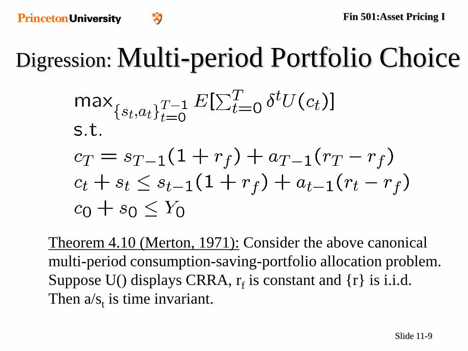
Digression: Multi-period Portfolio Choice

Theorem 4.10 (Merton, 1971): Consider the above canonical

multi-period consumption-saving-portfolio allocation problem.

Suppose U() displays CRRA, rf is constant and {r} is i.i.d.

Then a/st is time invariant.

Fin 501:Asset Pricing I

Slide 11-10

(Dynamic) Hedging Demand

• Illustration with noise trader risk:

Suppose fundamental value is constant v=1, but price is

noisy (due to noise traders)

If the asset is underpriced, e.g. p=.9 , then it might be

even more underpriced in the next period

• Myopic risk-averse investor:

buy some of the asset and push price towards 1, but not fully

• Forward-looking risk-averse investor:

yes, there can be intermediate losses if price declines in next

period, but then investment opportunity set improves even

more i.e. if returns are bad, then I have great opportunity

(dynamic hedge)

Fin 501:Asset Pricing I

Slide 11-11

Dynamic hedging demand

• Trade-off

Low return realization in next period

• Good since opportunity going forward is high

Invest more

Bad since marginal utility is high

Consume and invest less

High return realization in next period ….

• Utility

1 first (second) effect dominates

1(log-utility) both effects offset each other

Fin 501:Asset Pricing I

Slide 11-12

Conditional vs. unconditional CAPM

• If of each subperiod CAPM are time-

independent, then

conditional CAPM = unconditional CAPM

• If s are time-varying they may co-vary with Rm

and hence CAPM equation does not hold for

unconditional expectations.

Additional co-variance terms have to be considered!

Move from single-factor setting to multi-factor

setting