Lecture 1.1 CQF 2010_B

The Random Behaviour ofAssets

In this lecture. . .

• Different types of financial analysis

• Examining time-series data to model returns

• Are prices random?

• The need for probabilistic models

• The Wiener process, a mathematical model of randomness

• The lognormal random walk—The most important model forequities, currencies, commodities and indices

Certificate in Quantitative Finance

1

By the end of this lecture you will be able to

• analyze stock price data statistically

• understand and justify the lognormal random walk for assets

• explain where this simple model goes wrong


2

Introduction

In this lecture we start with some very simple analysis of equity

price data, and then using some common sense we build up a

discrete-time asset price model.

We often like to work in continuous time, so we will see how a

continuous-time model can be based on our discrete-time model.

This will be our first look at stochastic calculus and Wiener

processes. (This will be very important in most of the CQF!)


3

The three main types of ‘analysis’ used in finance

1. Fundamental Analysis

2. Technical Analysis

3. Quantitative Analysis


4

SP500

0

200

400

600

800

1000

1200

1400

1600

1800

12-Apr-49 29-Jun-57 15-Sep-65 02-Dec-73 18-Feb-82 07-May-90 24-Jul-98 10-Oct-06

The unpredictability that is seen in this figure is the most im-portant feature of financial modelling. Because there is so muchrandomness, the most successful mathematical models of finan-cial assets have a probabilistic foundation.


5

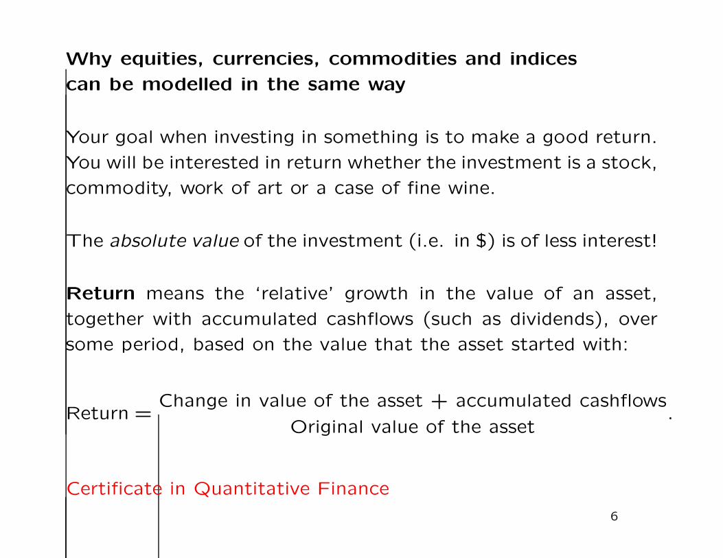
Why equities, currencies, commodities and indices

can be modelled in the same way

Your goal when investing in something is to make a good return.

You will be interested in return whether the investment is a stock,

commodity, work of art or a case of fine wine.

The absolute value of the investment (i.e. in $) is of less interest!

Return means the ‘relative’ growth in the value of an asset,

together with accumulated cashflows (such as dividends), over

some period, based on the value that the asset started with:

Return =Change in value of the asset + accumulated cashflows

Original value of the asset.


6

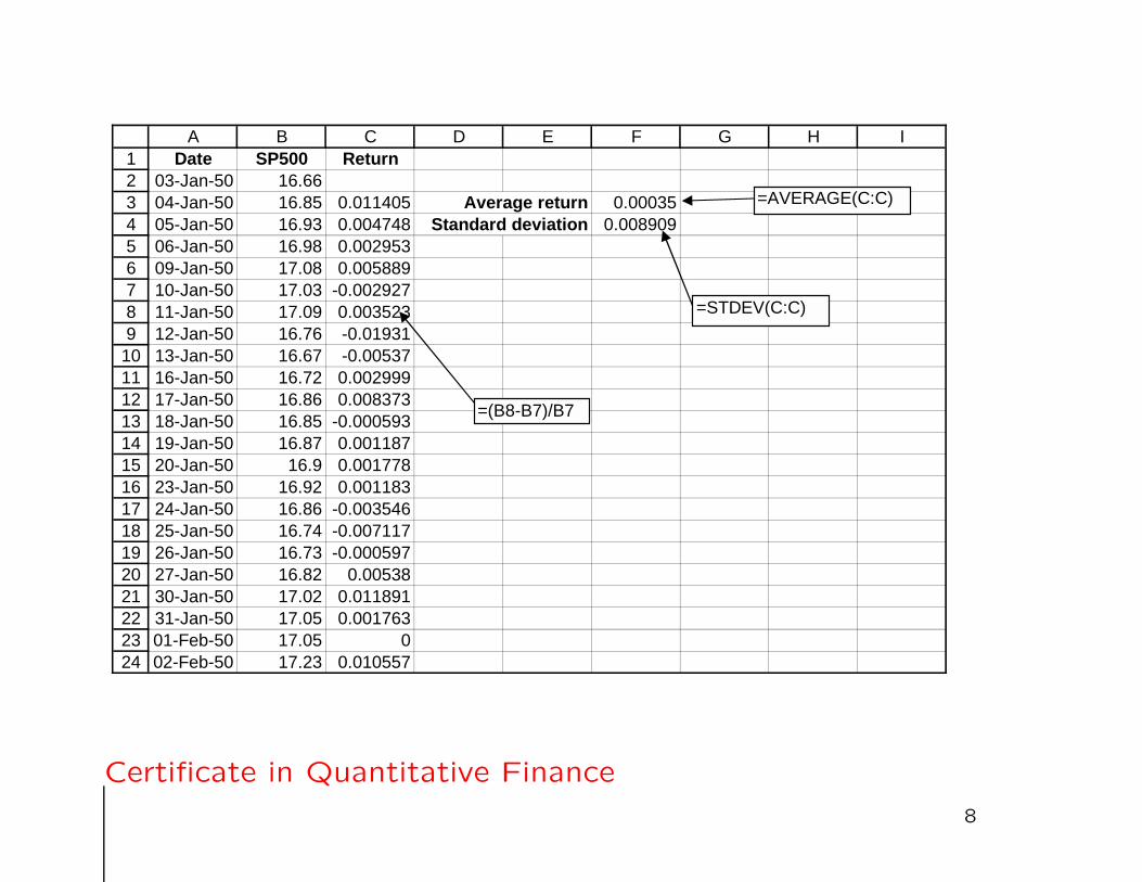
Examining returns

This suggests that instead of examining equity prices directly, we

should look at returns over some period.

Often one looks at returns over a period of a day.

If the asset value on the ith day is denoted by Si, then the return

from day i to day i+1 is given by

• Si+1 − Si

Si= Ri.

Let’s see this on a spreadsheet.


7

123456789

101112131415161718192021222324

A B C D E F G H IDate SP500 Return

03-Jan-50 16.6604-Jan-50 16.85 0.011405 Average return 0.0003505-Jan-50 16.93 0.004748 Standard deviation 0.00890906-Jan-50 16.98 0.00295309-Jan-50 17.08 0.00588910-Jan-50 17.03 -0.00292711-Jan-50 17.09 0.00352312-Jan-50 16.76 -0.0193113-Jan-50 16.67 -0.0053716-Jan-50 16.72 0.00299917-Jan-50 16.86 0.00837318-Jan-50 16.85 -0.00059319-Jan-50 16.87 0.00118720-Jan-50 16.9 0.00177823-Jan-50 16.92 0.00118324-Jan-50 16.86 -0.00354625-Jan-50 16.74 -0.00711726-Jan-50 16.73 -0.00059727-Jan-50 16.82 0.0053830-Jan-50 17.02 0.01189131-Jan-50 17.05 0.00176301-Feb-50 17.05 002-Feb-50 17.23 0.010557

=(B8-B7)/B7

=AVERAGE(C:C)

=STDEV(C:C)


8

This same data was used in the following plot of the daily returns

for S&P500 versus time. In the following pages we will model

the returns each day as random, and independent from one day

to the next.

SP500 returns

-0.25

-0.2

-0.15

-0.1

-0.05

0

0.05

0.1

0.15



9

The mean of the returns is

R̄ =1

M

M∑

i=1

Ri = AVERAGE( · )

and the sample standard deviation is

√√√√√ 1

M − 1M∑

i=1

(Ri − R̄)2 = STDEV( · ),

where M is the number of returns in the sample. (The expres-sions on the right are the Excel equivalents.)

From the data in this S&P500 example we find that the meanis 0.00035 and the standard deviation is 0.008909.


10

Now we know some numbers associated with the (random) re-

turn, but what about the shape of the distribution?

We are going to use the data to plot the probability density

function for returns. And then we will compare the result with a

very famous and important distribution.

But first we must standardize the distribution to give it a mean

of zero and a standard deviation of one.


11

How to normalize. . .

1234567891011121314151617

A B C D E F G HDate SP500 Return Scaled rtns

03-Jan-50 16.6604-Jan-50 16.85 0.011405 1.2408 Average return 0.0003505-Jan-50 16.93 0.004748 0.493593 Standard deviation 0.00890906-Jan-50 16.98 0.002953 0.29217209-Jan-50 17.08 0.005889 0.62172410-Jan-50 17.03 -0.002927 -0.36792411-Jan-50 17.09 0.003523 0.35613712-Jan-50 16.76 -0.01931 -2.20677513-Jan-50 16.67 -0.00537 -0.64209216-Jan-50 16.72 0.002999 0.29734317-Jan-50 16.86 0.008373 0.90053818-Jan-50 16.85 -0.000593 -0.10590819-Jan-50 16.87 0.001187 0.093920-Jan-50 16.9 0.001778 0.16027823-Jan-50 16.92 0.001183 0.09350524-Jan-50 16.86 -0.003546 -0.437372

=(C9-$G$3)/$G$4


12

And here is the distribution!

0

0.1

0.2

0.3

0.4

0.5

0.6

-4 -3 -2 -1 0 1 2 3 4

SP500Normal

The probability density function for the standardized Normal

distribution (also having zero mean and standard deviation of

one) is also shown:

• 1√2π

e−12φ2.

Why have I plotted the Normal (or Gaussian) distribution? Why

do we like it?


13

Assuming that the empirical returns can be modelled by a Normal

distribution then we have our first model!

With

• φ as a random variable drawn from a Gaussian distribution

our model will represent the returns as a random variable drawn

from a Normal distribution with a known, constant, non-zero

mean and a known, constant, non-zero standard deviation:

• Ri =Si+1 − Si

Si= 0.00035 + 0.008909 × φ.


14

More generally, i.e. for other indices than S&P500, or for stocks,

currencies, commodities, etc.,

• Ri =Si+1 − Si

Si= mean + standard deviation× φ.

This model has two, easily understood parameters.

Aside: Commodities may show seasonal behaviour, so the mean

and standard deviation may vary with time.


15

Goal: How can we get to a continuous-time model? At the

moment this model is in discrete time.

(Maths is easier in continuous time!)

Preliminary question: How do the parameters (the mean return

and the standard deviation) vary with the time step we are using

(here one day)?


16

Moving towards continuous time

We need to figure out how the mean and standard deviation of

the returns’ time series scale with the time step between asset

price measurements?

In our example the data is sampled with a time step of one day.

We could have used weekly or monthly intervals, or hourly (more

data needed, and harder to get). How would this affect the mean

and standard deviation?


17

How does the mean return scale with time?

If the average return in one day is 1%, what is the average return

over one week?


18

The average return scales with the size of the time step.

So the answer is 5% (if there are five business days in a week.)

Obvious!?


19

Let’s do the maths. . .

Call the time step δt. This is going to be a very small number,

a tiny fraction of a year.


20

I claim we can write

• mean = µ δt,

for some µ. (We will assume this to be constant, even if it’s notthe argument doesn’t change much.)

I.e. average return is proportional to the length of the periodover which it is measured..

In our S&P500 example we have

mean = 0.00035 = µ δt = µ × 1

252,

since there are approximately 252 business days in a year.

So µ = 0.0882 = 8.82%.


21

Ignoring randomness for the moment while we focus on the

mean, our model is simply

Si+1 − Si

Si= mean = µ δt.

This can be written as

Si+1 = Si(1 + µ δt).


22

If the asset begins at S0 at time t = 0 then after one time step

t = δt and

S1 = S0(1 + µ δt).

After two time steps t = 2 δt and

S2 = S1(1 + µ δt) = S0(1 + µ δt)2.

After M time steps t =M δt and

SM = S0(1 + µ δt)M.


23

But we can write

SM = S0 (1 + µ δt)M

as

S0eM log(1+µ δt)

because logarithms and exponentials are the inverses of each

other.


24

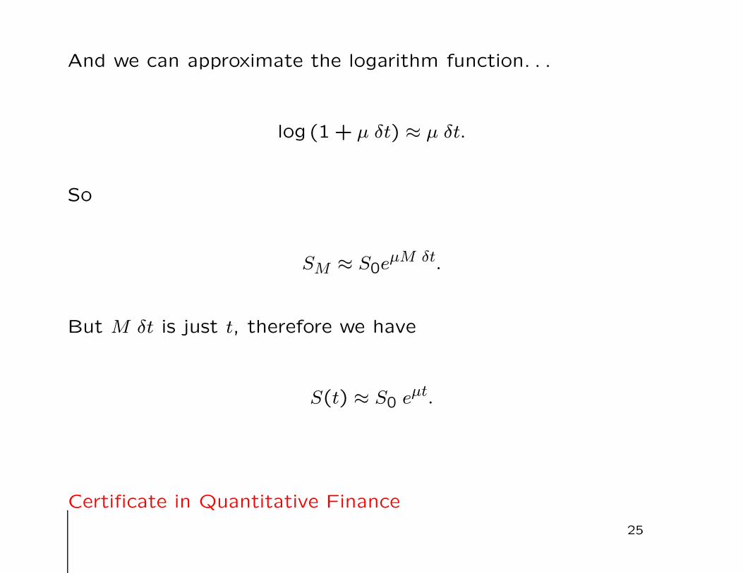
And we can approximate the logarithm function. . .

log (1 + µ δt) ≈ µ δt.

So

SM ≈ S0eµM δt.

But M δt is just t, therefore we have

S(t) ≈ S0 eµt.


25

In the limit as the time step δt → 0 S as a function of t becomes

S(t) = S0 eµt.

And there aren’t any δts in this! Which means that we have

something interesting and meaningful when the time step is in-

finitesimal.


26

This also shows why the answer to the question about the 1%

mean over one day etc. is only approximate. The scaling with

time step is actually exponential, it’s just that for small enough

periods things look linear.


27

Aside: What if the mean didn’t scale linearly with the time step?

What if instead

mean = µ δtα

with α �= 1? Go through the same analysis to see what happens!


28

• In the absence of any randomness the asset exhibits expo-nential growth, just like money in the bank.

• The model is meaningful in the limit as the time step tendsto zero.

To expand on the second point, had we chosen to scale the

mean of the returns distribution with any other power of δt

it would have resulted in either a boring model (S(t) = S0)

or a silly model, with infinite values for the asset.

µ is called the growth rate or drift rate.


29

Now let’s turn our attention to the standard deviation. . .


30

How does the standard deviation of returns scale with time?

If the standard deviation of returns is 1% over one day, what is

the standard deviation of returns over one week?

This one is not so obvious!


31

Clue: When you have independent random numbers (such as

returns from one day to the next) you cannot add standard de-

viations. Oh, no!

But you can add variances. I.e. when X and Y are independent

Var[X + Y ] = Var[X] + Var[Y ].

We will need this in what follows.


32

Let’s suppose that the standard deviation scales with δtα. There-

fore the variance scales with δt2α.

From time zero to time t how many random returns are there?

Easy, just t/δt.

So we have a number t/δt of variables each with variance of size

δt2α. Add up this many variances and you’ll get a total variance

from time zero to time t of size. . .


33

t

δt× δt2α.

We want to have a finite, non-zero, variance after a finite period

of time in the limit as δt → 0 therefore we must have

α = 12.

Therefore the standard deviation of returns scales with the square

root of the time step.


34

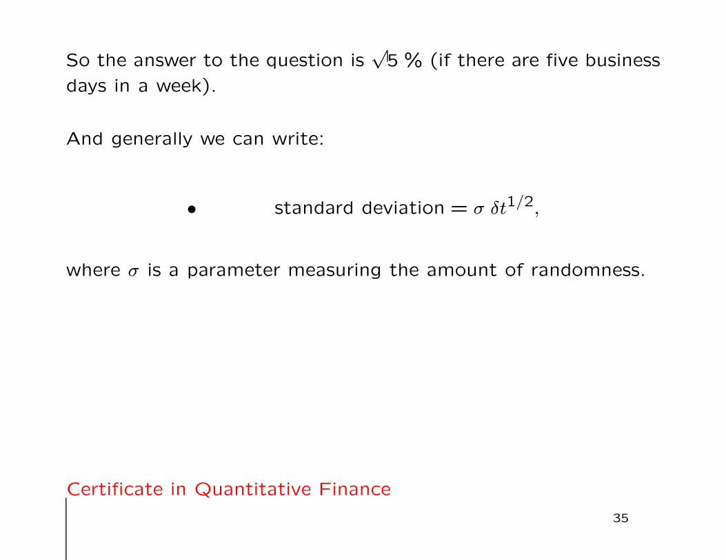
So the answer to the question is√5 % (if there are five business

days in a week).

And generally we can write:

• standard deviation = σ δt1/2,

where σ is a parameter measuring the amount of randomness.


35

σ is the volatility.

It is the annualized standard deviation of returns.


36

In our S&P500 example we have

standard deviation = 0.008909 = σ δt12 = σ × 1√

252.

So σ = 0.141 = 14.1%.


37

What units do the drift, µ, and the volatility, σ, have?


38

Back to the full model

Our asset return model, in words, is

Ri =Si+1 − Si

Si= mean + standard deviation× φ.

And using only symbols,

Ri =Si+1 − Si

Si= µ δt+ σφ δt1/2.


39

This can be written as

• Si+1 − Si = µSi δt+ σSiφ δt1/2. (1)

This is a model!

(But it is still in discrete time.)


40

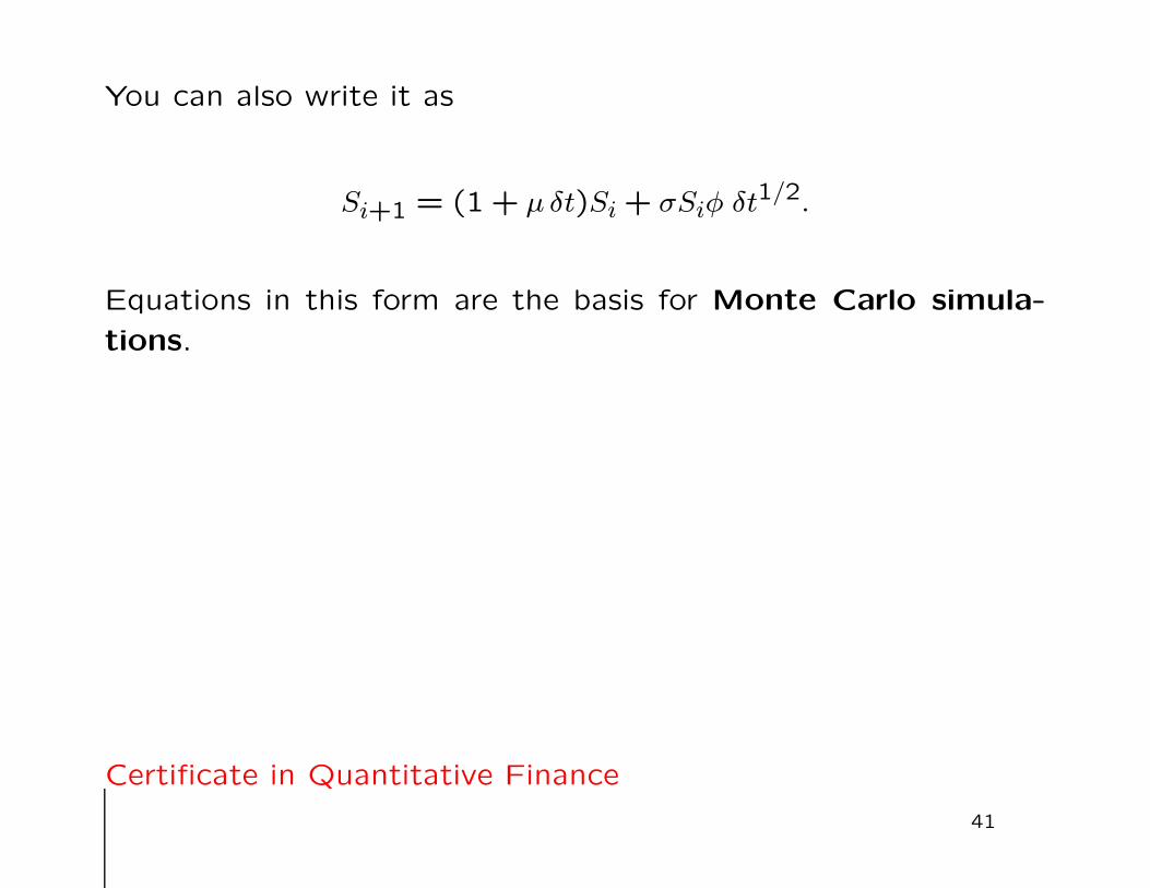
You can also write it as

Si+1 = (1+ µ δt)Si+ σSiφ δt1/2.

Equations in this form are the basis for Monte Carlo simula-

tions.


41

This is a discrete-time model for a random walk of the asset.

We know exactly where the asset price is today but tomorrow’s

value is unknown.


42

Because of their different scalings with time, the growth and

volatility have different effects on the asset path.

• The growth is not apparent over short timescales. Thevolatility dominates in the short term.

• Over long timescales, for instance decades, the growth be-comes important.


43

Ln(SP500)

0

1

2

3

4

5

6

7

8

9


Path of the logarithm of SP500, also showing its expected path(the straight line) and one standard deviation above and below

(parabolas).


44

The Wiener process

We have still not reached our goal of continuous time, we still

have a discrete time step.

We will now see a brief introduction to the continuous-time limit.

(You’ll be seeing the more rigorous side in later CQF lectures!)


45

We now introduce some more, very standard, notation: d· means‘the change in’ some quantity.

So dS is the ‘change in the asset price.’

But this change will be in continuous time.

• In effect, we will go to the limit δt = 0.


46

The first δt on the right-hand side of

Si+1 − Si = µSi δt+ σSiφ δt1/2.

becomes dt, but the second term is more complicated.


47

We cannot straightforwardly write dt1/2 instead of δt1/2.

Why not?


48

We are going to write the term φ δt1/2 as

dX.


49

You can think of dX as being a random variable, drawn from a

Normal distribution with mean zero and variance dt:

E[dX] = 0 and E[dX2] = dt.

This is not exactly what it is, but it is close enough to give the

right idea. (More later!)

• This is called a Wiener process.

We can build up a continuous-time theory using Wiener processes

instead of a discrete-time theory using Normal distributions.


50

The most important model for equities,

currencies, commodities and indices

Using the Wiener process notation, the asset price model can bewritten as

• dS = µS dt+ σS dX.

This is a stochastic differential equation (or sde). It is acontinuous-time model of an asset price.

It is the most widely accepted model for equities, currencies,commodities and indices, and the foundation of much financetheory.

(And sdes play a BIG role in all of quantitative finance!)


51

Summary

Please take away the following important ideas

• The return on an investment is the natural quantity to ana-lyze

• In finance theory this return is usually treated as being ran-dom

• The random return is often assumed to be Normally dis-tributed. This is not perfect but is a good starting point

• The asset price can then be modeled as a lognormal randomwalk

• This random walk is the most popular asset price model, andis in the form of a stochastic differential equation


52

Lecture 1.1 CQF 2010_B

Documents

Transcript of Lecture 1.1 CQF 2010_B