
Lecture 10: Partitioning Chi Squares and Residual...
30
Lecture 10: Partitioning Chi Squares and Residual Analysis Dipankar Bandyopadhyay, Ph.D. BMTRY 711: Analysis of Categorical Data Spring 2011 Division of Biostatistics and Epidemiology Medical University of South Carolina Lecture 10: Partitioning Chi Squares and Residual Analysis – p. 1/29
-
Upload
phungnguyet -
Category
Documents
-
view
216 -
download
0
Transcript of Lecture 10: Partitioning Chi Squares and Residual...
Lecture 10: Partitioning Chi Squares and Residual Analysis
Dipankar Bandyopadhyay, Ph.D.
BMTRY 711: Analysis of Categorical Data Spring 2011
Division of Biostatistics and Epidemiology
Medical University of South Carolina
Lecture 10: Partitioning Chi Squares and Residual Analysis – p. 1/29

Partitioning Chi-Squares
• We have developed tests of independence
• When a test of independence has a small p−value, what does it say about the strengthof the association?
• Not much, the smaller the p−value, the stronger the evidence that AN associationexists...i.e., you are more confident that X and Y are NOT independent.
• It does not tell you that the association is very strong.
• If you want to understand more about the association, you essentially have two optionsusing contingency tables: (1) a residual analysis and (2) consider partitioning theChi-Square statistics.
• We will develop a residual analysis similar to regression models in which we willcompare how close the observed values (the Oij ‘s) are to the expected values (theEij ‘s).
• We will also explore partitioning the likelihood ratio test into pieces to examineassociations in subtables (i.e., attempt to isolate the strongest trends)
Lecture 10: Partitioning Chi Squares and Residual Analysis – p. 2/29
Very General Method
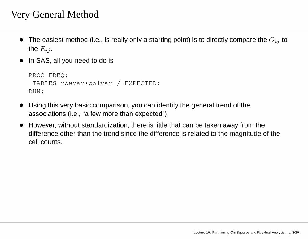
• The easiest method (i.e., is really only a starting point) is to directly compare the Oij tothe Eij .
• In SAS, all you need to do is
PROC FREQ;TABLES rowvar * colvar / EXPECTED;
RUN;
• Using this very basic comparison, you can identify the general trend of theassociations (i.e., “a few more than expected”)
• However, without standardization, there is little that can be taken away from thedifference other than the trend since the difference is related to the magnitude of thecell counts.
Lecture 10: Partitioning Chi Squares and Residual Analysis – p. 3/29

Example
Recall our ever popular MI example.
Myocardial InfarctionFatal Attack or NoNonfatal attack Attack
Placebo 189 10845
Aspirin 104 10933
Selected outputStatistic DF Value Prob--------------------------------------------------- ---Chi-Square 1 25.0139 <.0001Likelihood Ratio Chi-Square 1 25.3720 <.0001
We see strong evidence of an association.
Lecture 10: Partitioning Chi Squares and Residual Analysis – p. 4/29
Expected Counts Tabulated
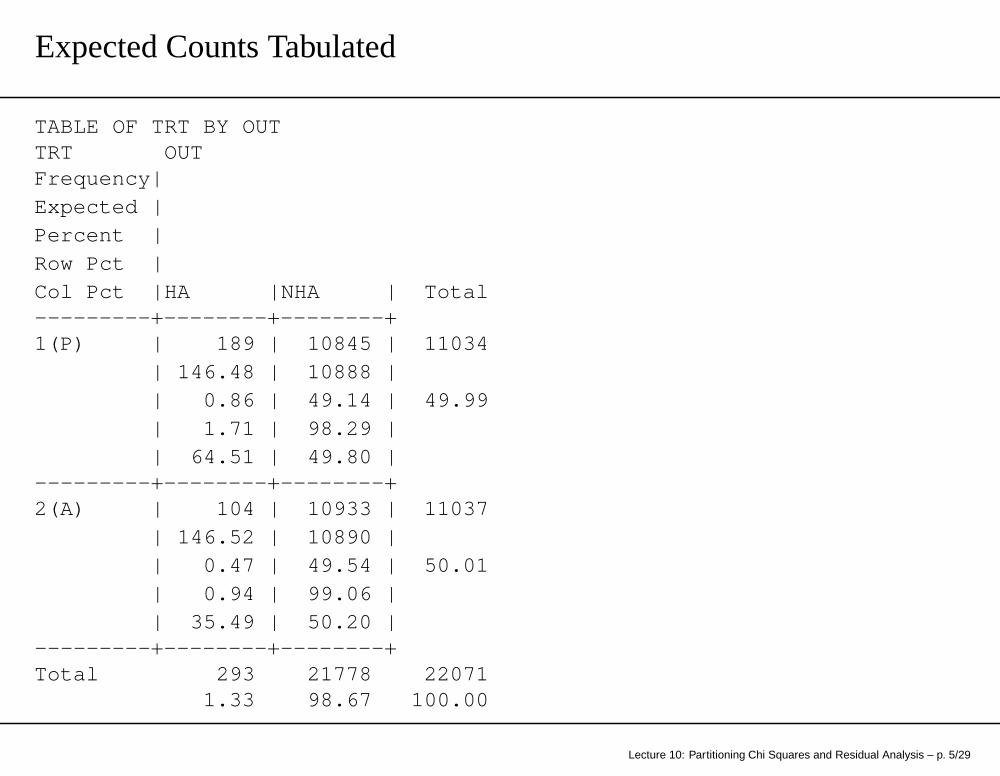
TABLE OF TRT BY OUTTRT OUTFrequency|Expected |Percent |Row Pct |Col Pct |HA |NHA | Total---------+--------+--------+1(P) | 189 | 10845 | 11034
| 146.48 | 10888 || 0.86 | 49.14 | 49.99| 1.71 | 98.29 || 64.51 | 49.80 |
---------+--------+--------+2(A) | 104 | 10933 | 11037
| 146.52 | 10890 || 0.47 | 49.54 | 50.01| 0.94 | 99.06 || 35.49 | 50.20 |
---------+--------+--------+Total 293 21778 22071
1.33 98.67 100.00
Lecture 10: Partitioning Chi Squares and Residual Analysis – p. 5/29
Pearson’s Residuals
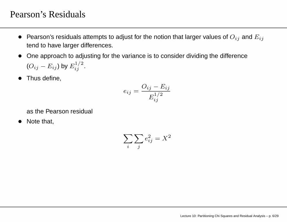
• Pearson’s residuals attempts to adjust for the notion that larger values of Oij and Eij
tend to have larger differences.
• One approach to adjusting for the variance is to consider dividing the difference
(Oij − Eij ) by E1/2
ij .
• Thus define,
eij =Oij − Eij
E1/2
ij
as the Pearson residual
• Note that,
X
i
X
j
e2
ij = X2
Lecture 10: Partitioning Chi Squares and Residual Analysis – p. 6/29

• Under H0, eij are asymptotically normal with mean 0.
• However, the variance of eij is less than 1.
• To compensate for this, one can use the STANDARDIZED Pearson Residuals.
• Denote esij as the standardized residuals in which
rij =Oij − Eij
(Eij(1 − pi·)(1 − p·j))1/2
where pi· = ni·/N is the estimated row i marginal probability
• rij is asymptotically distributed as a standard normal
Lecture 10: Partitioning Chi Squares and Residual Analysis – p. 7/29

Utilizing the Information
• As a “rule of thumb”, a rij value greater than 2 or 3 indicates a lack of fit of H0 in thatcell.
• However, as the number of cells increases, the likelihood that a cell has a value of 2 or3 increases. For example, if you have 20 cells, you could expect 1 in the 20 to have avalue greater the 2 just by chance (i.e., α = 0.05).
• Calculation of these residuals in not straight forward using PROC FREQ in SAS.
• PROC GENMOD using the RESIDUAL option produces the estimated residuals asReschi and Stdreschi automatically.
• We’ll begin covering GENMOD shortly, for now just consider the SAS code as anexample.
Lecture 10: Partitioning Chi Squares and Residual Analysis – p. 8/29
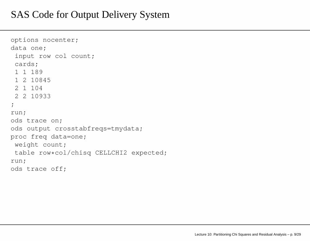
SAS Code for Output Delivery System
options nocenter;data one;
input row col count;cards;1 1 1891 2 108452 1 1042 2 10933
;run;ods trace on;ods output crosstabfreqs=tmydata;proc freq data=one;
weight count;table row * col/chisq CELLCHI2 expected;
run;ods trace off;
Lecture 10: Partitioning Chi Squares and Residual Analysis – p. 9/29
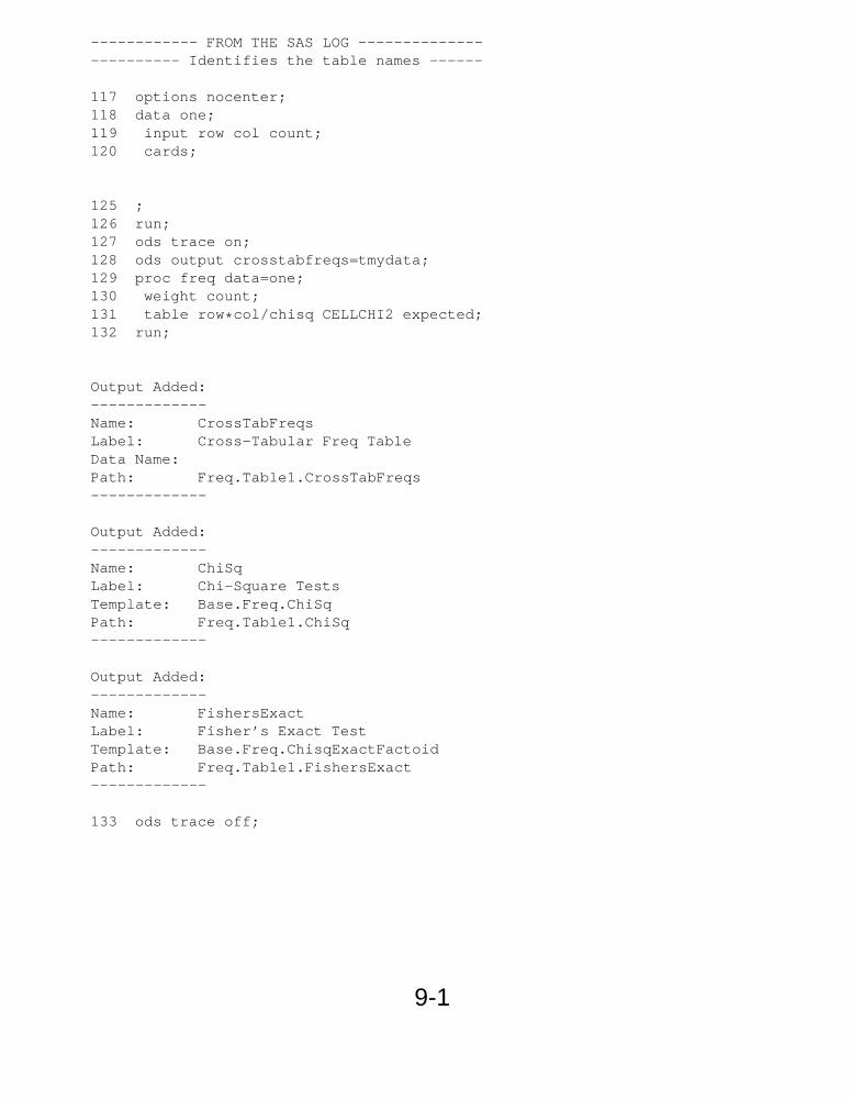
------------ FROM THE SAS LOG ------------------------ Identifies the table names ------
117 options nocenter;118 data one;119 input row col count;120 cards;
125 ;126 run;127 ods trace on;128 ods output crosstabfreqs=tmydata;129 proc freq data=one;130 weight count;131 table row * col/chisq CELLCHI2 expected;132 run;
Output Added:-------------Name: CrossTabFreqsLabel: Cross-Tabular Freq TableData Name:Path: Freq.Table1.CrossTabFreqs-------------
Output Added:-------------Name: ChiSqLabel: Chi-Square TestsTemplate: Base.Freq.ChiSqPath: Freq.Table1.ChiSq-------------
Output Added:-------------Name: FishersExactLabel: Fisher’s Exact TestTemplate: Base.Freq.ChisqExactFactoidPath: Freq.Table1.FishersExact-------------
133 ods trace off;
9-1
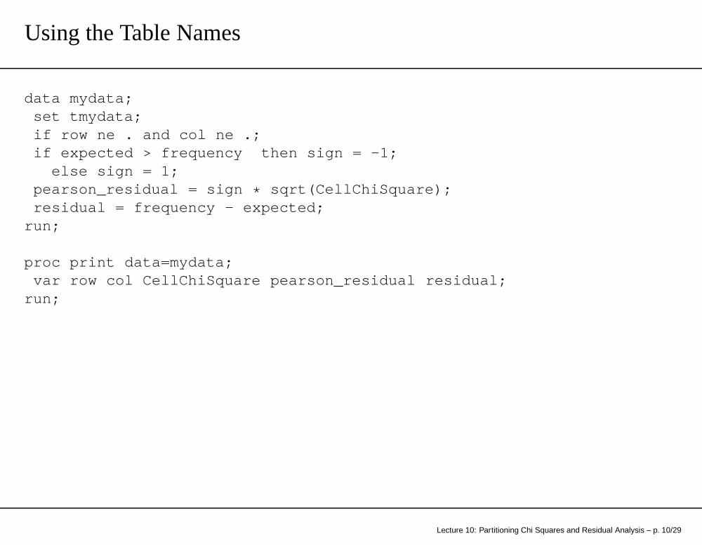
Using the Table Names
data mydata;set tmydata;if row ne . and col ne .;if expected > frequency then sign = -1;
else sign = 1;pearson_residual = sign * sqrt(CellChiSquare);residual = frequency - expected;
run;
proc print data=mydata;var row col CellChiSquare pearson_residual residual;
run;
Lecture 10: Partitioning Chi Squares and Residual Analysis – p. 10/29
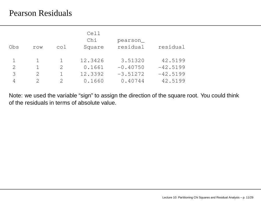
Pearson Residuals
CellChi pearson_
Obs row col Square residual residual
1 1 1 12.3426 3.51320 42.51992 1 2 0.1661 -0.40750 -42.51993 2 1 12.3392 -3.51272 -42.51994 2 2 0.1660 0.40744 42.5199
Note: we used the variable “sign” to assign the direction of the square root. You could thinkof the residuals in terms of absolute value.
Lecture 10: Partitioning Chi Squares and Residual Analysis – p. 11/29

Total ChiSquare
proc sql;create table totalchisq as select
sum(cellchisquare) as ChiSq
from mydata;
proc print data=totalchisq;run;
--------- Output ------------Obs ChiSq
1 25.0139
Lecture 10: Partitioning Chi Squares and Residual Analysis – p. 12/29

Regular PROC FREQ output
Statistic DF Value Prob--------------------------------------------------- ---Chi-Square 1 25.0139 <.0001Likelihood Ratio Chi-Square 1 25.3720 <.0001
Lecture 10: Partitioning Chi Squares and Residual Analysis – p. 13/29
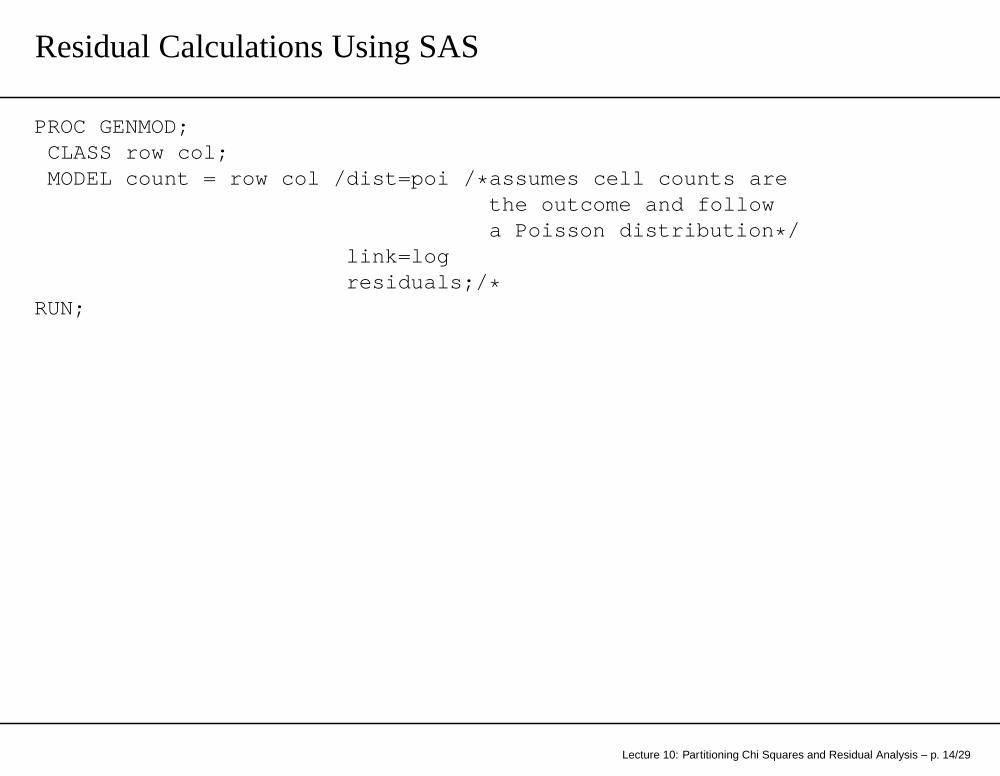
Residual Calculations Using SAS
PROC GENMOD;CLASS row col;MODEL count = row col /dist=poi / * assumes cell counts are
the outcome and followa Poisson distribution * /
link=logresiduals;/ *
RUN;
Lecture 10: Partitioning Chi Squares and Residual Analysis – p. 14/29
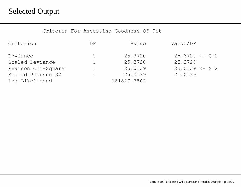
Selected Output
Criteria For Assessing Goodness Of Fit
Criterion DF Value Value/DF
Deviance 1 25.3720 25.3720 <- Gˆ2Scaled Deviance 1 25.3720 25.3720Pearson Chi-Square 1 25.0139 25.0139 <- Xˆ2Scaled Pearson X2 1 25.0139 25.0139Log Likelihood 181827.7802
Lecture 10: Partitioning Chi Squares and Residual Analysis – p. 15/29

Observation Statistics
Observation Resraw Reschi StReschi
1 42.519853 3.513196 5.00138022 -42.51991 -0.4075 -5.0013873 -42.51997 -3.512728 -5.0013944 42.519913 0.4074449 5.0013872
Here: Observation is in the order of the data set. To avoid confusion, instead of the option“residual”, you can use “obstat”.
Lecture 10: Partitioning Chi Squares and Residual Analysis – p. 16/29

Obstat Option
PROC GENMOD data=one;CLASS row col;MODEL count = row col /dist=poi / * assumes cell counts are
the outcome and followa Poisson distribution * /
link=logobstatsresiduals;
RUN;
Lecture 10: Partitioning Chi Squares and Residual Analysis – p. 17/29

Observation Statistics
Observation count row col Pred StdResraw Reschi StResdev
1 189 1 1 146.48015 0.058807242.519853 3.513196 4.784706
2 10845 1 2 10887.52 0.0095519-42.51991 -0.4075 -5.004648
3 104 2 1 146.51997 0.058807-42.51997 -3.512728 -5.278334
4 10933 2 2 10890.48 0.009550642.519913 0.4074449 4.998138
Note: I’ve cleaned up some of the output. Suggestion: Use obstat first to confirm the cells,then use residual to identify just the residuals of interest.
Lecture 10: Partitioning Chi Squares and Residual Analysis – p. 18/29

Partitioning the Likelihood Ratio Test
Motivation for this:
• If you reject the H0 and conclude that X and Y are dependent, the next questioncould be ‘Are there individual comparisons more significant than others?’.
• Partitioning (or breaking a general I × J contingency table into smaller tables) mayshow the association is largely dependent on certain categories or groupings ofcategories.
Recall, these basic principles about Chi Square variables
• If X1 and X2 are both (independently) distributed as χ2 with df = 1 then
• X = X1 + X2 ∼ χ2(df = 1 + 1)
• In general, the sum of independent χ2 random variables is distributed asχ2(df =
P
df(Xi))
Lecture 10: Partitioning Chi Squares and Residual Analysis – p. 19/29
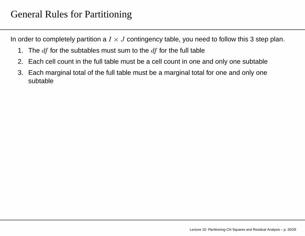
General Rules for Partitioning
In order to completely partition a I × J contingency table, you need to follow this 3 step plan.
1. The df for the subtables must sum to the df for the full table
2. Each cell count in the full table must be a cell count in one and only one subtable
3. Each marginal total of the full table must be a marginal total for one and only onesubtable
Lecture 10: Partitioning Chi Squares and Residual Analysis – p. 20/29
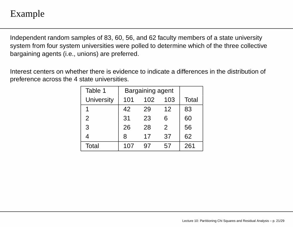
Example
Independent random samples of 83, 60, 56, and 62 faculty members of a state universitysystem from four system universities were polled to determine which of the three collectivebargaining agents (i.e., unions) are preferred.
Interest centers on whether there is evidence to indicate a differences in the distribution ofpreference across the 4 state universities.
Table 1 Bargaining agentUniversity 101 102 103 Total
1 42 29 12 832 31 23 6 603 26 28 2 564 8 17 37 62
Total 107 97 57 261
Lecture 10: Partitioning Chi Squares and Residual Analysis – p. 21/29
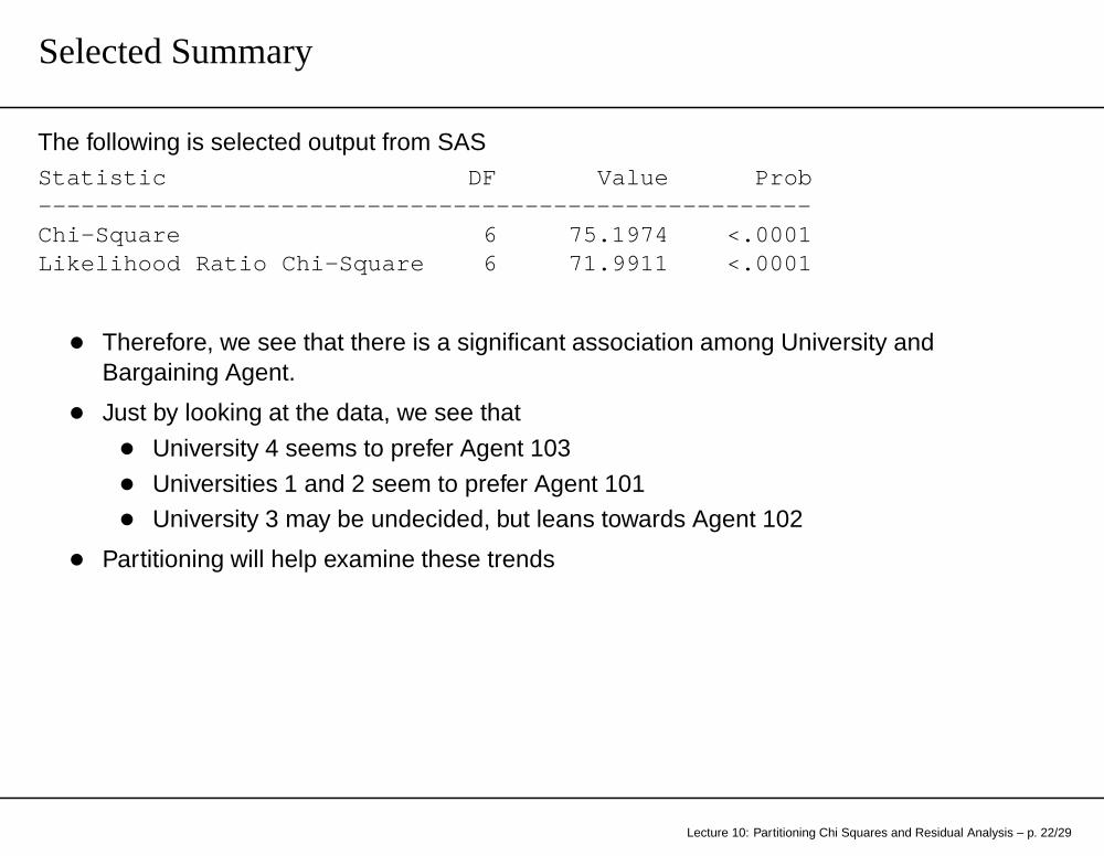
Selected Summary
The following is selected output from SASStatistic DF Value Prob--------------------------------------------------- ---Chi-Square 6 75.1974 <.0001Likelihood Ratio Chi-Square 6 71.9911 <.0001
• Therefore, we see that there is a significant association among University andBargaining Agent.
• Just by looking at the data, we see that
• University 4 seems to prefer Agent 103
• Universities 1 and 2 seem to prefer Agent 101
• University 3 may be undecided, but leans towards Agent 102
• Partitioning will help examine these trends
Lecture 10: Partitioning Chi Squares and Residual Analysis – p. 22/29

First subtable
The Association of University 4 appears the strongest, so we could consider a subtable of
Subtable 1 Bargaining AgentUniversity 101 and 102 103 Total
1 - 3 179 20 1994 25 37 62
Total 204 57 261
Note: This table was obtained by considering the {4, 3} cell in comparison to the rest of thetable.
G2 = 60.5440 on 1 df (p=0.0).
We see strong evidence for an association among universities (grouped accordingly) andagents.
Lecture 10: Partitioning Chi Squares and Residual Analysis – p. 23/29
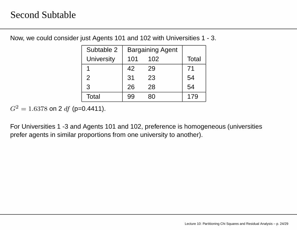
Second Subtable
Now, we could consider just Agents 101 and 102 with Universities 1 - 3.
Subtable 2 Bargaining AgentUniversity 101 102 Total
1 42 29 712 31 23 543 26 28 54
Total 99 80 179
G2 = 1.6378 on 2 df (p=0.4411).
For Universities 1 -3 and Agents 101 and 102, preference is homogeneous (universitiesprefer agents in similar proportions from one university to another).
Lecture 10: Partitioning Chi Squares and Residual Analysis – p. 24/29
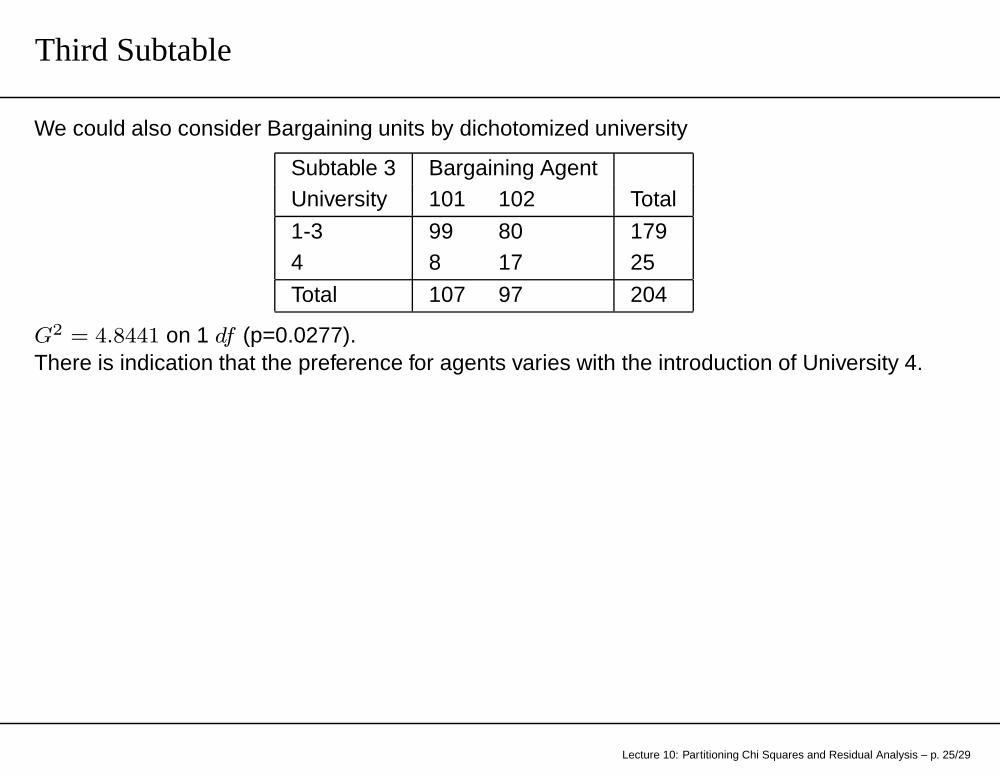
Third Subtable
We could also consider Bargaining units by dichotomized university
Subtable 3 Bargaining AgentUniversity 101 102 Total
1-3 99 80 1794 8 17 25
Total 107 97 204
G2 = 4.8441 on 1 df (p=0.0277).There is indication that the preference for agents varies with the introduction of University 4.
Lecture 10: Partitioning Chi Squares and Residual Analysis – p. 25/29
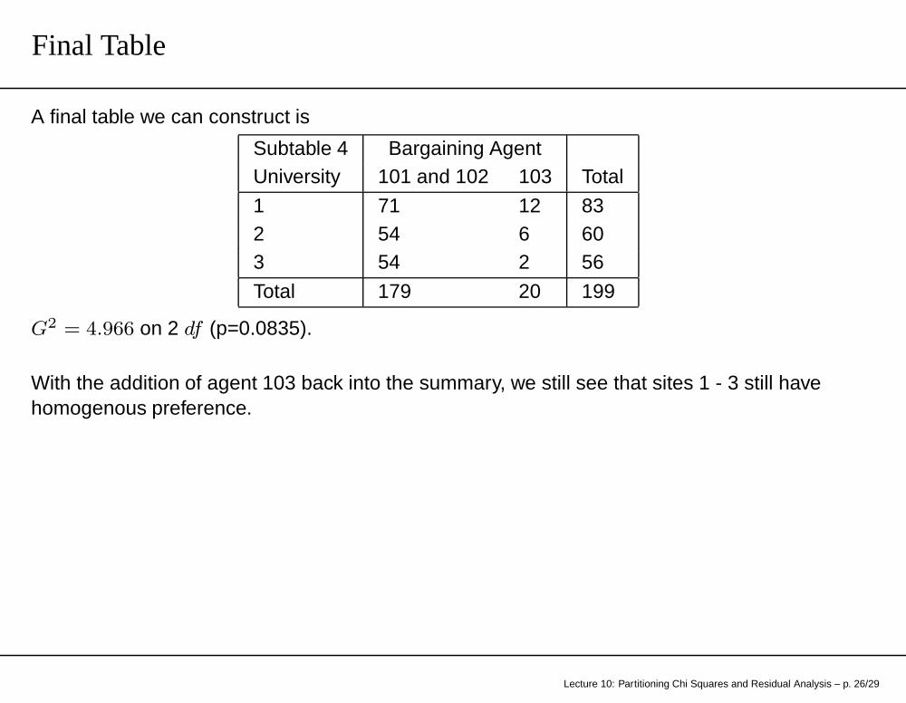
Final Table
A final table we can construct is
Subtable 4 Bargaining AgentUniversity 101 and 102 103 Total
1 71 12 832 54 6 603 54 2 56
Total 179 20 199
G2 = 4.966 on 2 df (p=0.0835).
With the addition of agent 103 back into the summary, we still see that sites 1 - 3 still havehomogenous preference.
Lecture 10: Partitioning Chi Squares and Residual Analysis – p. 26/29
What have we done?
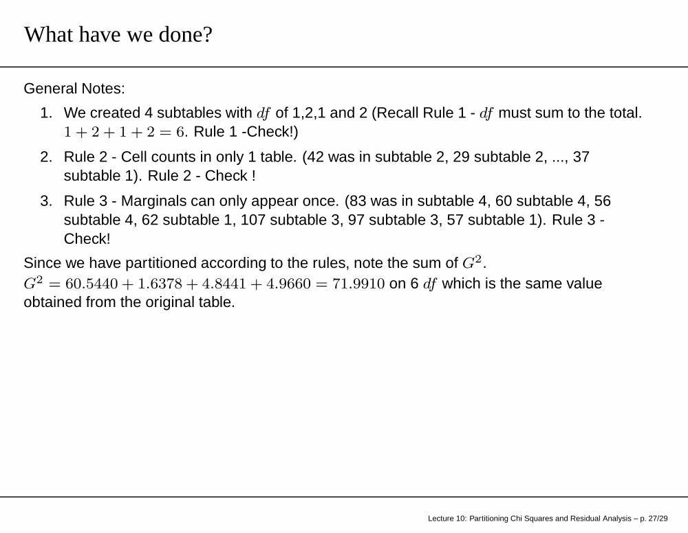
General Notes:
1. We created 4 subtables with df of 1,2,1 and 2 (Recall Rule 1 - df must sum to the total.1 + 2 + 1 + 2 = 6. Rule 1 -Check!)
2. Rule 2 - Cell counts in only 1 table. (42 was in subtable 2, 29 subtable 2, ..., 37subtable 1). Rule 2 - Check !
3. Rule 3 - Marginals can only appear once. (83 was in subtable 4, 60 subtable 4, 56subtable 4, 62 subtable 1, 107 subtable 3, 97 subtable 3, 57 subtable 1). Rule 3 -Check!
Since we have partitioned according to the rules, note the sum of G2.G2 = 60.5440 + 1.6378 + 4.8441 + 4.9660 = 71.9910 on 6 df which is the same valueobtained from the original table.
Lecture 10: Partitioning Chi Squares and Residual Analysis – p. 27/29
Overall Summary of Example
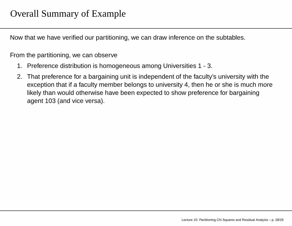
Now that we have verified our partitioning, we can draw inference on the subtables.
From the partitioning, we can observe
1. Preference distribution is homogeneous among Universities 1 - 3.
2. That preference for a bargaining unit is independent of the faculty’s university with theexception that if a faculty member belongs to university 4, then he or she is much morelikely than would otherwise have been expected to show preference for bargainingagent 103 (and vice versa).
Lecture 10: Partitioning Chi Squares and Residual Analysis – p. 28/29
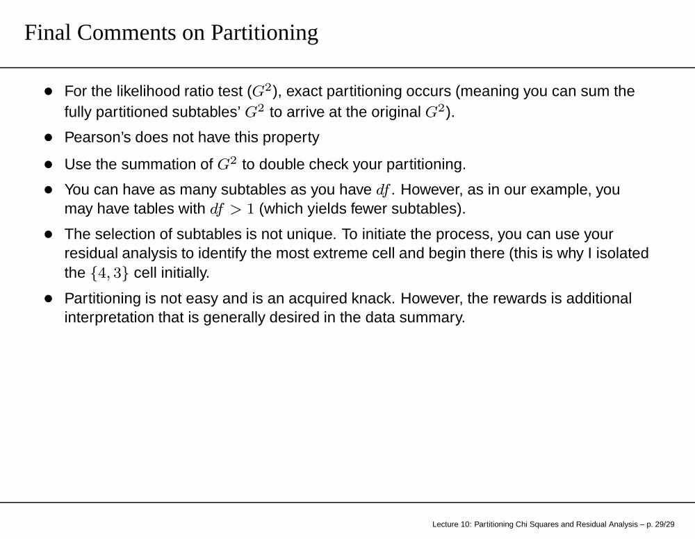
Final Comments on Partitioning
• For the likelihood ratio test (G2), exact partitioning occurs (meaning you can sum thefully partitioned subtables’ G2 to arrive at the original G2).
• Pearson’s does not have this property
• Use the summation of G2 to double check your partitioning.
• You can have as many subtables as you have df . However, as in our example, youmay have tables with df > 1 (which yields fewer subtables).
• The selection of subtables is not unique. To initiate the process, you can use yourresidual analysis to identify the most extreme cell and begin there (this is why I isolatedthe {4, 3} cell initially.
• Partitioning is not easy and is an acquired knack. However, the rewards is additionalinterpretation that is generally desired in the data summary.
Lecture 10: Partitioning Chi Squares and Residual Analysis – p. 29/29


![Residual Tide analysis in shallow waTeR - …...Tidal analysis For the tidal analysis the classical least squares harmonic approach is preferred over the response method [7] – due](https://static.fdocuments.in/doc/165x107/5f387bd3163dad3d5169160b/residual-tide-analysis-in-shallow-water-tidal-analysis-for-the-tidal-analysis.jpg)


![Least Squares Methods for Elliptic Systems* · 2018. 11. 16. · the least squares residual in the boundary condition. The paper [5] has an historical importance for the following](https://static.fdocuments.in/doc/165x107/6034e184bf2df84b66377553/least-squares-methods-for-elliptic-systems-2018-11-16-the-least-squares-residual.jpg)


