Lecture 1 Measures of Informationhomepage.ntu.edu.tw/~ihwang/Teaching/Fa16/Slides/... · Lecture1...

Lecture 1Measures of Information

I-Hsiang Wang

Department of Electrical EngineeringNational Taiwan University

[email protected]

September 20, 2016

1 / 61 I-Hsiang Wang IT Lecture 1

mailto:[email protected]

How to measure information?

Before this, we should ask:

What is information?


In daily lives, information is often obtained by learning something unknown before.

Examples: result of a ball game, score of an exam, weather, …

In other words, one gets some information by learning something about which that he/shewas uncertain before.

Shannon: "Information is the resolution of uncertainty."


Motivating Example

Let us take the following example:Suppose there is a professional basketball (NBA) final and a tennis tournament (the FrenchOpen quarterfinals) happening right now.

D is an enthusiastic sports fan. He is interested in who will win the NBA final and who will winthe Men's single.

However, due to his work, he cannot access any news in 10 days.

How much information can he get after 10 days when he learns the two pieces of news (the twomessages)?

For the NBA final, D will learn that one of the two teams eventually wins the final (message B).

For the French Open quarterfinals, D will learn that one of the eight players eventually wins the goldmedal (message T).


Observations

1 The amount of information is related to the number of possible outcomes: message B is a resultof two possible outcomes, while message T is a result of eight possible outcomes.

2 The amount of information obtained in learning the two messages should be additive, while thenumber of possible outcomes is multiplicative.

Let f (·) be a function that measures the amount of information:

f (·)

f (·)

# of possible outcomes of B

# of possible outcomes of T

Amount of info. from learning B

Amount of info. from learning T

f (·)

# of possible outcomes of B

# of possible outcomes of T

Amount of info. from learning B

Amount of info. from learning T

⇥ +

What function produces additive outputs with multiplicative inputs? Logarithmic Function


Logarithm as the Information Measure

Initial guess of the measure of information: log (# of possible outcomes).

However, this measure does not take the likeliness into account -- if some outcome occurs with veryhigh probability, the amount of information of that outcome should be very little.

For example, suppose D knows that the Spurs was leading the Heats 3:1The probability that the Heats win the final: 1

2 → 18 .

The Heats win the final (w.p. 18 ): it is like out of 8 times there is only 1 time that will generate this

outcome =⇒ the amount of information = log 8 = 3 bits.

The probability that the Spurs win the final: 12 → 7

8 .The Spurs win the final (w.p. 7

8 ): it is like out of 87 times there is only 1 time that will generate this

outcome =⇒ the amount of information = log 87 = 3− log 7 bits.


Information and Uncertainty

From the motivation, we collect the following intuitions:1 The amount of information is related to the # of possible outcomes2 The measure of information should be additive3 The measure of information should take the likeliness into account4 The measure of information = The amount of uncertainty of an unknown outcome

Hence, a plausible measure of information of a realization x drawn from a random outcome X is

f (x) ≜ log 1P{X=x} .

Correspondingly, the measure of information of a random outcome X is the averaged value of f (x):

EX [f(X)] .

(in this lecture, the logarithms are of base 2 if not specified.)


Entropy and Conditional Entropy

1 Entropy and Conditional EntropyDefinitionsProperties

2 Mutual InformationDefinitionsProperties

3 Information DivergenceDefinitionsProperties



Entropy: Measure of Uncertainty of a Random Variable

log 1P{X=x} : measure of information/uncertainty of an outcome x.

If the outcome has small probability, it contains higher uncertainty. However, on the average, ithappens rarely. Hence, to measure the uncertainty of a random variable, we should take theexpectation of the self information over all possible realizations:

Definition 1 (Entropy)

The entropy of a (discrete) random variable X ∈ X with probability mass function PX (·) is defined as

H (X ) ≜ EX

[log 1

PX(X)

]=∑x∈X

PX(x) log 1PX(x) .

(by convention we set 0 log(1/0) = 0 since limt→0 t log t = 0.)

Note: Entropy can be understood as the (average) amount of information when one learns the actualoutcome/realization of r.v. X .



Example 1 (Binary entropy function)

Let X ∼ Ber(p) be a Bernoulli random variable,that is, X ∈ {0, 1}, PX(1) = 1− PX(0) = p,p ∈ [0, 1]. Then, the entropy of X is called thebinary entropy function Hb(p), where

Hb(p) ≜ H (X ) = −p log p− (1− p) log(1− p).

Exercise 11 Analytically check that

maxp∈[0,1]

Hb(p) = 1, arg maxp∈[0,1]

Hb(p) = 1/2.

2 Analytically prove that Hb(p) is concave in p.

1.2 Uncertainty or Entropy 9

p

Hb(p)[bits]

0 0.1 0.2 0.3 0.4 0.5 0.6 0.7 0.8 0.9 10

0.1

0.2

0.3

0.4

0.5

0.6

0.7

0.8

0.9

1

Figure 1.2: Binary entropy function Hb(p) as a function of the probabilityp.

Definition 1.9. If U is binary with two possible values u1 and u2, U ={u1, u2}, such that Pr[U = u1] = p and Pr[U = u2] = 1− p, then

H(U) = Hb(p) (1.27)

where Hb(·) is called the binary entropy function and is defined as

Hb(p) ! −p log2 p− (1− p) log2(1− p), p ∈ [0, 1]. (1.28)

The function Hb(·) is shown in Figure 1.2.

Exercise 1.10. Show that the maximal value of Hb(p) is 1 bit and is takenon for p = 1

2 . ♦

1.2.3 The Information Theory Inequality

The following inequality has not really a name, but since it is so importantin information theory, we will follow Prof. James L. Massey, retired professorat ETH in Zurich, and call it the information theory inequality or the ITinequality.

Proposition 1.11 (IT Inequality). For any base b > 0 and any ξ > 0,!1− 1

ξ

"logb e ≤ logb ξ ≤ (ξ − 1) logb e (1.29)

with equalities on both sides if, and only if, ξ = 1.

Proof: Actually, Figure 1.3 can be regarded as a proof. For thosereaders who would like a formal proof, we provide next a mathematicalderivation. We start with the upper bound. First note that

logb ξ##ξ=1

= 0 = (ξ − 1) logb e##ξ=1

. (1.30)

c⃝ Copyright Stefan M. Moser, version 2.7, Fall Semester 2012/2013

p0 0.5 1

0

0.5

1Hb(p)



Example 2

Consider a random variable X ∈ {0, 1, 2, 3} with p.m.f. defined as follows:

x 0 1 2 3

P (x) 16

13

13

16

Compute H (X ) and H (Y ), where Y ≜ X mod 2.

sol:H (X ) = 2× 1

6 × log 6 + 2× 13 × log 3 = 1

3 + log 3.H (Y ) = 2× 1

2 × log 2 = 1.

(when the context is clear, we drop the subscripts in PX , PY , PY |X , etc.)



Operational Meaning of Entropy

Besides the intuitive motivation, Entropy has operational meanings.Below we take a slight deviation and look at a mathematical problem.

♢

Problem: Consider a sequence of discrete rv's Xn ≜ (X1, X2, . . . , Xn), where

Xi ∈ X , Xii.i.d.∼ PX , ∀ i = 1, 2, . . . , n. |X | < ∞.

For a given ϵ ∈ (0, 1), we say B ⊆ X n is an ϵ-high-probability set iff

P {Xn ∈ B} ≥ 1− ϵ.

Goal: Find the asymptotic size of the smallest ϵ-high-probability set as n → ∞.



Theorem 1 (Cardinality of High Probability Sets)

Let s (n, ϵ) be the size of the smallest ϵ-high-probability set. Then,limn→∞

1n log s (n, ϵ) = H (X ) , ∀ ϵ ∈ (0, 1).

pf: Application of Law of Large Numbers.

Implications: H (X ) is the minimum possible compression ratio.With the theorem, if one would like to describe a random length-n X-sequence with a missedprobability at most ϵ, he/she only needs k ≈ nH (X ) bits when n is large.

Why? Because the above theorem guarantees that, for any prescribed missed probability,1n × (minimum # of bits required) → H (X ) as n → ∞.

This is the saving (compression) due to the statistical structure of random source sequences!(as Shannon pointed out in his 1948 paper.)


Entropy and Conditional Entropy Definitions






Entropy: Definition

Initially we define entropy for a random variable; it is straightforward to extend this definition to asequence of random variables, or, a random vector.

The entropy of a random vector is also called the joint entropy of the component random variables.

Definition 2 (Entropy)

The entropy of a d-dimensional random vector X ≜[X1 · · · Xd

]⊺ is defined by the expectationof the self information

H (X ) ≜ EX

[log 1

PX(X)

]=

∑X∈X1×···×Xd

PX(X) log 1PX(X) = H (X1, . . . , Xd ) .

Remark: Entropy of a rv. is a function of the distribution of the rv.. Hence, we often write H (P ) andH (X ) interchangeably for a rv. X ∼ P .



Example 3

Consider two random variables X1, X2 ∈ {0, 1} with joint p.m.f.

(x1, x2) (0, 0) (0, 1) (1, 0) (1, 1)

P (x1, x2)16

13

13

16

Compute H (X1 ), H (X2 ), and H (X1, X2 ).

sol:H (X1, X2 ) = 2× 1

6 × log 6 + 2× 13 × log 3 = 1

3 + log 3.H (X1 ) = 2×

(13 + 1

6

)× log 1

13+ 1

6

= 1 = H (X2 ) .

Compared to Example 2, it can be understood that the value of entropy only depends on thedistribution of the random variable/vector, not on the actual values it may take.



Conditional Entropy

For two r.v.'s with conditional p.m.f. PX|Y (x|y), we are able to define "the entropy of X givenY = y" according to PX|Y (·|y):

H (X |Y = y ) ≜∑x∈X

PX|Y (x|y) log 1PX|Y (x|y) .

H (X |Y = y ): the amount of uncertainty of X when we know that Y takes value at y.

Averaging over Y , we obtain the amount of uncertainty of X given Y :

Definition 3 (Conditional Entropy)

The conditional entropy of X given Y is defined by

H (X |Y ) ≜∑y∈Y

PY (y)H (X |Y = y ) =∑

x∈X ,y∈YPX,Y (x, y) log 1

PX|Y (x|y) = EX,Y

[log 1

PX|Y (X|Y )

].



Example 4


(x1, x2) (0, 0) (0, 1) (1, 0) (1, 1)

P (x1, x2)16

13

13

16

Compute H (X1 |X2 = 0 ), H (X1 |X2 = 1 ), H (X1 |X2 ), and H (X2 |X1 ).

sol: (x1, x2) (0, 0) (0, 1) (1, 0) (1, 1)

P (x1|x2) 13

23

23

13

P (x2|x1) 13

23

23

13

H (X1 |X2 = 0 ) = 13 log 3 + 2

3 log 32 = Hb

(13

), H (X1 |X2 = 1 ) = 2

3 log 32 + 1

3 log 3 = Hb(13

).

H (X1 |X2 ) = 2× 16 × log 3 + 2× 1

3 × log 32 = Hb

(13

)= log 3− 2

3 = H (X2 |X1 )


Entropy and Conditional Entropy Properties






Properties of Entropy

Theorem 2 (Properties of (Joint) Entropy)

1 H (X ) ≥ 0, with equality iff X is deterministic.

2 H (X ) ≤ log |X |, with equality iff X is uniformly distributed over X .

3 H (X ) ≥ 0, with equality iff X is deterministic.

4 H (X ) ≤∑d

i=1 log |Xi|, with equality iff X is uniformly distributed over X1 × · · · × Xd.

Interpretation: Quite natural:

Amount of uncertainty in X = 0 ⇐⇒ X is deterministic.

Amount of uncertainty in X is maximized ⇐⇒ X is equally likely to take every value in X .



Lemma 1 (Jensen's Inequality)

f : R → R be a strictly concave function, and X be a real-valued r.v.. Then, E [f(X)] ≤ f (E [X]),with equality iff X is deterministic.

We shall use the above lemma to prove that H (X ) ≤ log |X |, with equality iff X ∼ Unif [X ].

pf: Let the support of X , suppX , denote the subset of X where X takes non-zero probability.

Define a new r.v. U ≜ 1PX(X) . Note that E [U ] = |suppX |. Hence,

H (X ) = E [logU ](Jensen)≤ log (E [U ]) = log |suppX | ≤ log |X |.

The first inequality holds with equality iff U is deterministic iff ∀x ∈ suppX , PX(x) are equal.

The second inequality holds with equality iff suppX = X .

Exercise 2For any jointly distributed (X,Y ), show that H (X |Y ) ≥ 0 with equality iff X is a deterministic function of Y .



Chain Rule

Theorem 3 (Chain Rule)

H (X,Y ) = H (Y ) +H (X |Y ) = H (X ) +H (Y |X ).

Interpretation: Amount of uncertainty of (X,Y ) = Amount of uncertainty of Y + Amount ofuncertainty of X after knowing Y .

pf: By definition, H (X,Y ) =∑x∈X

∑y∈Y

P (x, y) log 1P (x,y) =

∑x∈X

∑y∈Y

P (x, y) log 1P (y)P (x|y)

=∑x∈X

∑y∈Y

P (x, y) log 1P (y) +

∑x∈X

∑y∈Y

P (x, y) log 1P (x|y)

= H (Y ) +H (X |Y )

(when the context is clear, we drop the subscripts in PX , PY , PY |X , etc.)



Conditioning Reduces Entropy

Theorem 4 (Conditioning Reduces Entropy)

H (X |Y ) ≤ H (X ), with equality iff X is independent of Y .

Interpretation: The more one learns, the less the uncertainty is.The amount of uncertainty of your target remains the same if and only if what you have learned isindependent of your target.

Exercise 3While it is always true that H (X |Y ) ≤ H (X ), for y ∈ Y , the following two are both possible:

H (X |Y = y ) < H (X ), or

H (X |Y = y ) > H (X ).

Please construct examples for the above two cases respectively.



pf: By definition and Jensen's inequality, we have

H (X |Y )−H (X )

=∑x∈X

∑y∈Y

P (x, y) log P (x)P (x|y) =

∑x∈X

∑y∈Y

P (x, y) log P (x)P (y)P (x,y)

≤ log( ∑

x∈X

∑y∈Y

P (x, y) P (x)P (y)P (x,y)

)= log

( ∑x∈X

∑y∈Y

P (x)P (y)

)= log (1) = 0



Example 5


(x1, x2) (0, 0) (0, 1) (1, 0) (1, 1)

P (x1, x2)16

13

13

16

In the previously examples, we have

H (X1, X2 ) = log 3 + 13 , H (X1 ) = H (X2 ) = 1,

H (X1 |X2 ) = H (X2 |X1 ) = log 3− 23 .

It is straightforward to check that the chain rule holds. Besides, it can be easily seen thatconditioning reduces entropy.



Generalization

Proofs of the more general "Chain Rule" and "Conditioning Reduces Entropy" are left as exercises.

Theorem 5 (Chain Rule)

The chain rule can be generalized to more than two r.v.'s:

H (X1, . . . , Xn ) =n∑

i=1H (Xi |X1, . . . , Xi−1 ).

Theorem 6 (Conditioning Reduces Entropy)

Conditioning reduces entropy can be generalized to more than two r.v.'s:H (X |Y, Z ) ≤ H (X |Y ).



Upper Bound on Joint Entropy

Corollary 1 (Joint Entropy ≤ Sum of Marginal Entropies)

H (X1, . . . , Xn ) ≤n∑

i=1H (Xi )

Proof is left as exercise (chain rule of entropy + conditioning reduces entropy).

Exercise 4Show that

H (X,Y, Z ) ≤ H (X,Y ) +H (X,Z )−H (X ) .



Concavity of Entropy

Theorem 7 (Concavity of Entropy)

Let p ≜[p1 · · · pm

]denote the p.m.f. vector of a random variable X . Then, the entropy of X ,

H (p ), is concave in p, where H (p ) ≜ −∑m

i=1 pi log pi. (written as H (p ) since it is a function of p)

pf: We would like to show that for any λ ∈ [0, 1], λ = 1− λ,

H(λp1 + λp2

)≥ λH (p1 ) + λH (p2 ) .

Setting X1 ∼ p1, X2 ∼ p2, and Θ with P {Θ = 1} = λ = 1− P {Θ = 2}.=⇒ H (XΘ ) ≥ H (XΘ |Θ ) since conditioning reduces entropy.

Noting XΘ ∼ pλ ≜ λp1 + λp2, and H (XΘ |Θ = i ) = H (pi ) for i = 1, 2, proof complete.

(we often use p and P (·) interchangeably to denote a pmf (vectors))


Mutual Information





Mutual Information

Conditioning Reduces Entropy Revisited

Entropy quantifies the amount of uncertainty of a r.v., say, X .

Conditional entropy quantifies the amount of uncertainty of a r.v. X given another r.v., say, Y .

H (X)

0

Learning Y

0

H (X|Y )

Question: How much information does Y tell about X?


Mutual Information

Conditioning Reduces Entropy Revisited

Entropy quantifies the amount of uncertainty of a r.v., say, X .

Conditional entropy quantifies the amount of uncertainty of a r.v. X given another r.v., say, Y .

H (X)

0

Learning Y

0

H (X|Y )

}I (X;Y )

Question: How much information does Y tell about X?

Ans: The amount of information about X that one obtains by learning Y is H (X )−H (X |Y ).


Mutual Information Definitions






Mutual Information

Definition 4 (Mutual Information)

For a pair of jointly distributed r.v.'s (X,Y ), themutual information between them is defined as

I (X ;Y ) ≜ H (X )−H (X |Y ).

Relate: what channel coding does is to infersome information about the channel input X fromthe channel output Y .

H (X)

0

Learning Y

0

H (X|Y )

}I (X;Y )

PY |X (y|x)X Y



An Indentity about Mutual Information

Theorem 8 (An Identity)

I (X ;Y ) = H (X )−H (X |Y )

= H (Y )−H (Y |X )

= H (X ) +H (Y )−H (X,Y ) .

pf: By chain rule: H (X |Y ) = H (X,Y )−H (Y ).

(H (X,Y )

(

(

H (X)

H (Y )

H (Y |X) H (X|Y )

I (X;Y )Note: Mutual information is symmetric, that is, I (X ;Y ) = I (Y ;X ).

Note: The mutual information between X and itself is equal to its entropy: I (X ;X ) = H (X )



Mutual Information Measures the Level of Dependency

Theorem 9 (Extremal Values of Mutual Information)

1 I (X ;Y ) ≥ 0, with equality iff X,Y are independent.

2 I (X ;Y ) ≤ H (X ), with equality iff X is a deterministic function of Y .

pf: The proof of the first one is due to the fact that conditioning reduces entropy. The proof of thesecond one is due to H (X |Y ) ≥ 0.

Interpretation: the mutual information between X and Y , I (X ;Y ) can also be viewed as ameasure of the dependency between X and Y :

If X is determined by Y (highly dependent), I (X ;Y ) is maximized.If X is independent of Y (no dependency), I (X ;Y ) = 0.



Example 6


(x1, x2) (0, 0) (0, 1) (1, 0) (1, 1)

P (x1, x2)16

13

13

16

Compute I (X1 ;X2 ).

sol: From the previous examples, we have

H (X1, X2 ) = log 3 + 1

3, H (X1 ) = H (X2 ) = 1,

H (X1 |X2 ) = H (X2 |X1 ) = log 3− 2

3.

Hence, I (X1 ;X2 ) = H (X1 )−H (X1 |X2 ) =53 − log 3.



Conditional Mutual Information

Definition 5 (Conditional Mutual Information)

For a tuple of jointly distributed r.v.'s (X,Y, Z), the mutual information between X and Y given Z isI (X ;Y |Z ) ≜ H (X |Z )−H (X |Y, Z ).

Similar to the previous identity (Theorem 8), we have

I (X ;Y |Z ) = H (X |Z )−H (X |Y, Z ) = H (Y |Z )−H (Y |X,Z )

= H (X |Z ) +H (Y |Z )−H (X,Y |Z ) .

Similar to Theorem 9, we have1 I (X ;Y |Z ) ≥ 0, with equality iff X,Y are independent given Z (X −Z − Y forms a Markov chain).

2 I (X ;Y |Z ) ≤ H (X |Z ), with equality iff X is a deterministic function of Y and Z.


Mutual Information Properties






Chain Rule for Mutual Information

Theorem 10 (Chain Rule for Mutual Information)

I (X ;Y1, . . . , Yn ) =n∑

i=1

I (X ;Yi |Y1, . . . , Yi−1 ) .

pf: Proved by definition and the chain rule for entropy.

Exercise 5Show that I (X ;Z ) ≤ I (X ;Y,Z ) and I (X ;Y |Z ) ≤ I (X ;Y, Z ).



Data Processing Inequality

Theorem 11 (Data Processing Decreases Mutual Information)

For a Markov chain X − Y − Z (PX,Y,Z = PX · PY |X · PZ|Y ), I (X ;Y ) ≥ I (X ;Z ).

Interpretation: The Markov chain X − Y − Z implies that the information of X that Z can provideis contained in Y . Hence, the amount of information of X that can be inferred by Z ≤ the amount ofinformation of X that can be inferred by Y .

pf: Since X − Y − Z, we have I (X ;Z |Y ) = 0. Hence,

I (X ;Y, Z ) = I (X ;Y ) + I (X ;Z |Y ) = I (X ;Y ) (∵ I (X ;Z |Y ) = 0)

I (X ;Y, Z ) = I (X ;Z ) + I (X ;Y |Z ) (Chain Rule)=⇒ I (X ;Y ) = I (X ;Z ) + I (X ;Y |Z ) ≥ I (X ;Z ) .



Data Processing Inequality: Applications

Markov chains are common in communication systems. For example, in channel coding (withoutfeedback), the message W , the channel input XN ≜ X[1 : N ], the channel output Y N ≜ Y [1 : N ],and the decoded message W form a Markov chain W −XN − Y N − W ,

Encoder Noisy Channel DecoderW

X[1 : N ] Y [1 : N ]cW

pY |X

Data processing inequality is crucial in obtaining impossibility results in information theory.

Exercise 6 (Functions of R.V.)

For Z ≜ g (Y ) being a deterministic function of Y , show that H (Y ) ≥ H (Z ) and I (X ;Y ) ≥ I (X ;Z )

Exercise 7Show that X1 −X2 −X3 −X4 =⇒ I (X1 ;X4 ) ≤ I (X2 ;X3 ).



Example 7

Consider two random variables X1, X2 ∈ {0, 1} with the same joint p.m.f. as that in Example 6. LetX3 ≜ X2 ⊕ Z, where Z ∼ Ber (p) and Z is independent of (X1, X2).

1 Compute I (X1 ;X3 ) and I (X1 ;X2 |X3 ).2 Show that X1 −X2 −X3 forms a Markov chain.3 Verify the data processing inequality I (X1 ;X2 ) ≥ I (X1 ;X3 ).

sol:(x1, x2, x3) (0, 0, 0) (0, 0, 1) (0, 1, 0) (0, 1, 1)

P (x1, x2, x3)16 (1− p) 1

6p13p

13 (1− p)

(x1, x2, x3) (1, 0, 0) (1, 0, 1) (1, 1, 0) (1, 1, 1)

P (x1, x2, x3)13 (1− p) 1

3p16p

16 (1− p)

Then it is straightforward to compute mutual informations and verify the Markov chain.



Conditioning Reduces Mutual Information?

Does conditioning reduce mutual information? Does conditioning reduce the dependency?The answer is yes and no: sometimes yes, and sometimes no.

Example 8 (Conditioning Increases Mutual Information)

Let X,Y be i.i.d. Ber(1

2)

and Z ≜ X ⊕ Y . Find I (X ;Y |Z ) and show I (X ;Y |Z ) > I (X ;Y ).

sol: I (X ;Y |Z ) = H (X |Z )−H (X |Y, Z ) = H (X |Z )−H (X |Y,X ⊕ Y )= H (X |Z )−H (X |Y,X ) = H (X |Z ) = H (X ) = 1. (X ⊥⊥ Z )

On the other hand, I (X ;Y ) = 0. Hence, 1 = I (X ;Y |Z ) > I (X ;Y ) = 0.

Corollary 2 (Conditioning Decreases Mutual Information)

For a Markov chain X − Y − Z, we have I (X ;Y ) ≥ I (X ;Y |Z ).



Convexity and Concavity of Mutual Information

The convexity/concavity properties of mutual information turns out to be very useful in computingchannel capacity and rate distortion functions, as we will see in later lectures.

Theorem 12Let (X,Y ) ∼ PX,Y = PX · PY |X .

With PY |X fixed, I (X ;Y ) is a concave function of PX .With PX fixed, I (X ;Y ) is a convex function of PY |X .

pf: Refer to Section 2.7 of Cover&Thomas.


Information Divergence






Measuring the Distance between Probability Distributions

Recall that mutual information I (X;Y ) measures the dependency between two r.v.'s X and Y .

Reason: I (X;Y ) = E[log 1

PX(X)PY (Y ) − log 1PX,Y (X,Y )

], where the first term inside E [·]

measures the uncertainty of (X,Y ) when they are independent (with distribution PX · PY ), while thesecond term measures the actual uncertainty of (X,Y ) (with distribution PX,Y ).

In other words, it measures how far the independent distribution PX · PY is away from the actualdistribution PX,Y , in terms of uncertainty.

Information Divergence (Kullback–Leibler divergence) is a generalization of this concept, whichmeasures how far a distribution Q is away from the actual distribution P .


Information Divergence Definitions







Definition 6 (Information Divergence (Kullback–Leibler Divergence, Relative Entropy))

Let P (·) and Q (·) be two p.m.f.'s of a random variable X . The information divergence from Q to Pis

D (P ∥Q) ≜ EX∼P

[log P (X)

Q(X)

]=∑

x∈suppP P (x) log P (x)Q(x) .

Remarks:Above we follow the convention that 0 log 0

q = 0 ∀ 0 ≤ q ≤ 1, and p log p0 = ∞ ∀ 0 < p ≤ 1.

Hence, if the support of Q is strictly contained in the support of P , then D (P ∥Q) = ∞.

I (X;Y ) = D (PX,Y ∥PX · PY ).

Information divergence is NOT symmetric: D (P ∥Q) = D (Q ∥P ).



Example 9 (Binary divergence function)

Let p =[1− p p

]and q =

[1− q q

], p, q ∈ (0, 1). Then, the divergence from q to p is called

the binary divergence function db (p ∥q), where

db (p ∥q) ≜ D (p ∥q) = p log pq + (1− p) log (1−p)

(1−q) .

0 0.1 0.2 0.3 0.4 0.5 0.6 0.7 0.8 0.9 10

0.2

0.4

0.6

0.8

1

1.2

1.4

1.6

1.8

0 0.1 0.2 0.3 0.4 0.5 0.6 0.7 0.8 0.9 10

1

2

3

4

5

6

7

Exercise 8Prove the following statements.

1 db(p∥∥ 1

2

)= 1− Hb (p).

2 db (p ∥q) is convex in (p, q).

3 db (p ∥q) ≥ 2(p− q)2 log(e).



Operational Meaning of Information Divergence

KL divergence characterizes the asymptotic behavior of error probability in hypothesis testing.

♢

Problem (Hypothesis Testing): Consider a sequence of discrete rv's Xn ≜ (X1, X2, . . . , Xn), where

Xi ∈ X , Xii.i.d.∼ PX , ∀ i = 1, 2, . . . , n. |X | < ∞.

Goal: Design a good decision making algorithm to test which hypothesis of the following two is true,by observing the realization of Xn:{

H0 : PX = P0, that is, Xii.i.d.∼ P0

H1 : PX = P1, that is, Xii.i.d.∼ P1



Probability of Errors: Let us define two kinds of error probabilities:

Probability of miss detection: P(n)M ≜ P {H0 is chosen|H1}.

Probability of false alarm: P(n)F ≜ P {H1 is chosen|H0}.

Usually, one would like to minimize P(n)M while keeping P(n)

F below a prescribed threshold ϵ. Define

β (n, ϵ) ≜ minall testing algo. with P(n)

F ≤ ϵ

{P(n)M

}.

Theorem 13 (Chernoff-Stein)

limn→∞

− 1n logβ (n, ϵ) = D (P0 ∥P1) , ∀ ϵ ∈ (0, 1) .

Implications: The optimal probability of miss detection scales like 2−nD(P0 ∥P1), and the informationdivergence from P1 to P0 governs the rate of decay as n → ∞.



Conditional Information Divergence

Definition 7 (Conditional Information Divergence)

Let PY |X (·|·) and QY |X (·|·) be two conditional p.m.f.'s of random variables (X,Y ). Theconditional information divergence from QY |X to PY |X conditioned on PX (·) is

D(PY |X

∥∥QY |X∣∣PX

)≜ EX∼PX

[D(PY |X (·|X)

∥∥QY |X (·|X))]

=∑

(x,y)∈suppPX,YPX,Y (x, y) log PX|Y (x|y)

QX|Y (x|y) .

Exercise 9Prove the following identity: for (X,Y ) ∼ PX,Y = PX · PY |X = PY · PX|Y ,

I (X ;Y ) = D (PX,Y ∥PX · PY ) = D(PY |X

∥∥PY

∣∣PX

)= D

(PX|Y

∥∥PX

∣∣PY

).


Information Divergence Properties






Non-negativity of Information Divergence

Theorem 14D (P ∥Q) ≥ 0, with equality iff P (x) = Q (x) for all x ∈ X .

pf: Proved by Jensen's inequality similar to previous proofs.

Note: Although it is tempting to think of information divergence as a distance function, in fact it isnot, because (1) it is asymmetric, and (2) it does not satisfy the triangle inequality.

Exercise 10Show that uniform distribution attains maximal entropy, byusing D (P ∥Unif) ≥ 0, where Unif denotes the uniformdistribution over the alphabet.

Exercise 11 (Nonnegativity of Conditional Divergence)

ProveD

(PY |X

∥∥QY |X∣∣PX

)≥ 0.



Chain Rule for Information Divergence

Theorem 15 (Chain Rule for Information Divergence)

D (PX,Y ∥QX,Y ) = D(PY |X

∥∥QY |X∣∣PX

)+D (PX ∥QX)

D (PXn ∥QXn) =n∑

i=1D(PXi|Xi−1

∥∥QXi|Xi−1

∣∣PXi−1

)

pf: Proved by definition and the telescoping factorization of joint probability.

Exercise 12If QXn is a product distribution, that is , QXn =

∏ni=1 QXi . Show that

D (PXn ∥QXn) = D(PXn

∥∥∏ni=1 PXi

)+

∑ni=1 D (PXi ∥QXi) .



Convexity of Information Divergence

Theorem 18D (p ∥q) is convex in the pair (p, q).

pf: Refer to Section 2.7 of Cover&Thomas – a direction application of Log Sum Inequality (below).

Lemma 2 (Log Sum Inequality)

For sequences {ai ≥ 0 | i = 1, 2, . . . , n} and {bi ≥ 0 | i = 1, 2, . . . , n}, we have∑ni=1 ai log ai

bi≥ (∑n

i=1 ai) log∑n

i=1 ai∑ni=1 bi

,

with equality iff ∀ i, aibi

= constant.

pf: Let αi ≜ ai∑nj=1 ai

and βi ≜ bi∑nj=1 bi

. Hence, α ≜ [αi]ni=1 and β ≜ [βi]

ni=1 are valid p.m.f.

vectors. Proof is complete by D (α ∥β) ≥ 0, the nonnegativity of information divergence.


Summary


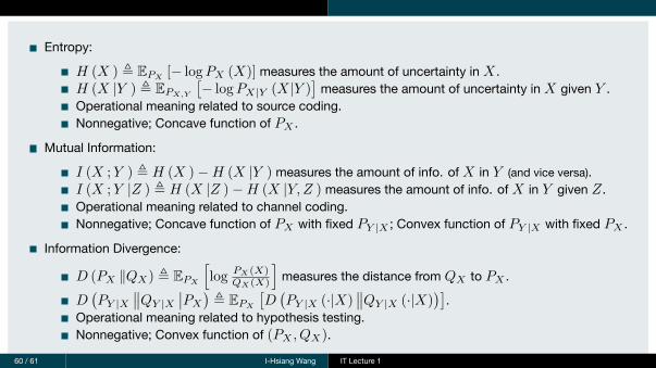
Entropy:

H (X ) ≜ EPX [− logPX (X)] measures the amount of uncertainty in X .H (X |Y ) ≜ EPX,Y

[− logPX|Y (X|Y )

]measures the amount of uncertainty in X given Y .

Operational meaning related to source coding.Nonnegative; Concave function of PX .

Mutual Information:

I (X ;Y ) ≜ H (X )−H (X |Y ) measures the amount of info. of X in Y (and vice versa).I (X ;Y |Z ) ≜ H (X |Z )−H (X |Y, Z ) measures the amount of info. of X in Y given Z.Operational meaning related to channel coding.Nonnegative; Concave function of PX with fixed PY |X ; Convex function of PY |X with fixed PX .

Information Divergence:

D (PX ∥QX) ≜ EPX

[log PX(X)

QX(X)

]measures the distance from QX to PX .

D(PY |X

∥∥QY |X∣∣PX

)≜ EPX

[D(PY |X (·|X)

∥∥QY |X (·|X))]

.Operational meaning related to hypothesis testing.Nonnegative; Convex function of (PX , QX).


Chain rule:

Entropy: H (Xn ) =∑n

i=1 H(Xi

∣∣Xi−1)

Mutual Information: I (X ;Y n ) =∑n

i=1 I(X ;Yi

∣∣Y i−1)

Information Divergence: D (PXn ∥QXn) =∑n

i=1 D(PXi|Xi−1

∥∥QXi|Xi−1

∣∣PXi−1

)Conditioning:

Conditioning reduces entropy: H (X |Y,Z ) ≤ H (X |Y )Conditioning may reduce mutual information: X − Y − Z =⇒ I (X ;Y |Z ) ≤ I (X ;Y )Conditioning increases divergence: D

(PY |X ◦ PX

∥∥QY |X ◦ PX

)≤ D

(PY |X

∥∥QY |X∣∣PX

).

Data processing:

Data processing decreases mutual information: X − Y − Z =⇒ I (X;Y ) ≥ I (X;Z).Data processing decreases divergence: D (PX ∥QX) ≥ D

(PX ◦ PY |X

∥∥QX ◦ PY |X).


Lecture 1 Measures of Informationhomepage.ntu.edu.tw/~ihwang/Teaching/Fa16/Slides/... · Lecture1...

Documents

Transcript of Lecture 1 Measures of Informationhomepage.ntu.edu.tw/~ihwang/Teaching/Fa16/Slides/... · Lecture1...