Aerodynamics

Lecture 1:

Introduction - Equations of

Motion

G. Dimitriadis

Definition

• Aerodynamics is the science that analyses the flow of air around solid bodies

• The basis of aerodynamics is fluid dynamics

• Aerodynamics only came of age after the first aircraft flight by the Wright brothers

• The primary driver of aerodynamics progress is aerospace and more particularly aeronautics

Applications (1)

Basic phenomena:

Flow around a cylinder

Shock wave Flow around an airfoil

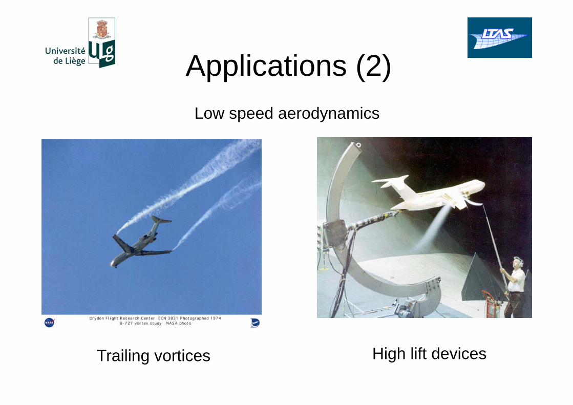
Applications (2)

Trailing vortices High lift devices

Low speed aerodynamics

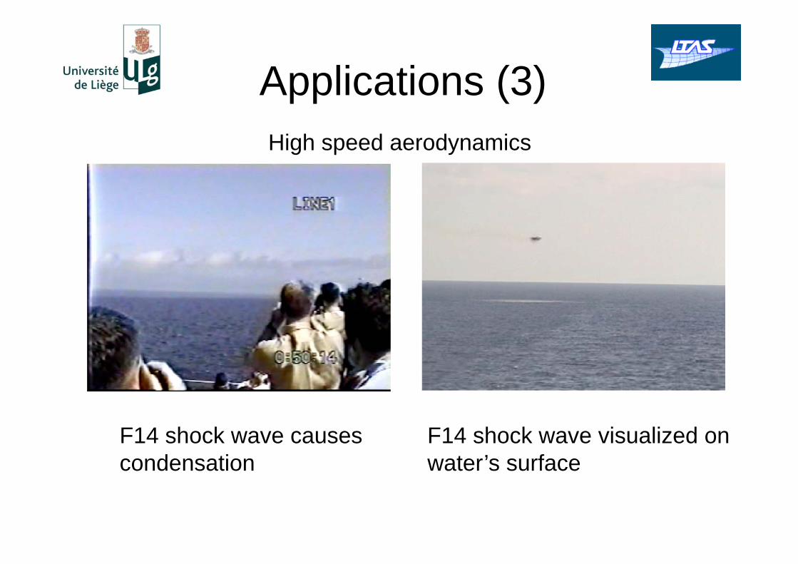
Applications (3)

High speed aerodynamics

F14 shock wave causes

condensation

F14 shock wave visualized on

water’s surface

Applications (4)

New concepts:

Blended wing body

Micro-air vehicles Forward-swept wings

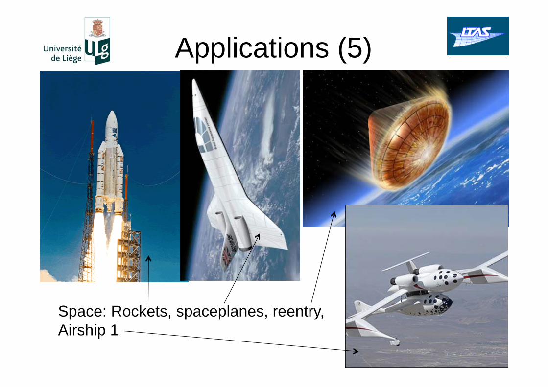
Applications (5)

Space: Rockets, spaceplanes, reentry,

Airship 1

Applications (6)

Non-aerospace applications: cars,

buildings, birds, insects

Categories of aerodynamics

• Aerodynamics is an all-encompassing term

• It is usually sub-divided according to the speed of the flow regime under investigation: – Subsonic aerodynamics: The flow is subsonic over

the entire body

– Transonic aerodynamics: The flow is sonic or supersonic over some parts of the body but subsonic over other parts

– Supersonic aerodynamics: The flow is supersonic over all of the body

– Hypersonic aerodynamics: The flow is faster than four times the speed of sound over all of the body

Flow type applications

• Subsonic aerodynamics: – Low speed aircraft, high-speed aircraft flying at

low speeds, wind turbines, environmental flows etc

• Transonic aerodynamics: – Aircraft flying at nearly the speed of sound,

helicopter rotor blades, turbine engine blades etc

• Supersonic aerodynamics: – Aircraft flying at supersonic speeds, turbine engine

blades etc

• Hypersonic aerodynamics: – Atmospheric re-entry vehicles, experimental

hypersonic aircraft, bullets, ballistic missiles, space launch vehicles etc

Content of this course (1)

• This course will address mostly

subsonic and supersonic aerodynamics

• Transonic aerodynamics is very difficult

and highly nonlinear

– Small perturbation linearized solutions exist

but their accuracy is debatable

• Hypersonic aerodynamics is beyond the

scope of this course

Content of this course (2)

• Subsonic aerodynamics – Incompressible aerodynamics

• Ideal flow – 2D flow

– 3D flow

• Viscous flow – Viscous-inviscid matching

– Compressibility corrections

• Supersonic aerodynamics – 2D flow

– 3D flow

Simplifications

• The different categories of aerodynamics exist because of the different amount of simplifications that can be applied to particular flows

• Air molecules always obey the same laws, irrespective of the size or speed of the object that is passing through them

• However, the way we analyze flows changes with flow regime because we apply simplifications

• Without simplifications very few useful results can be obtained

Full Navier Stokes Equations

• The most complete model we have of the flow of air is the Navier Stokes equations

• These equations are nevertheless a model: they are not the physical truth

• They represent three conservation laws: mass, momentum and energy

• They are not the physical truth because they involve a number of statistical quantities such as viscosity and density

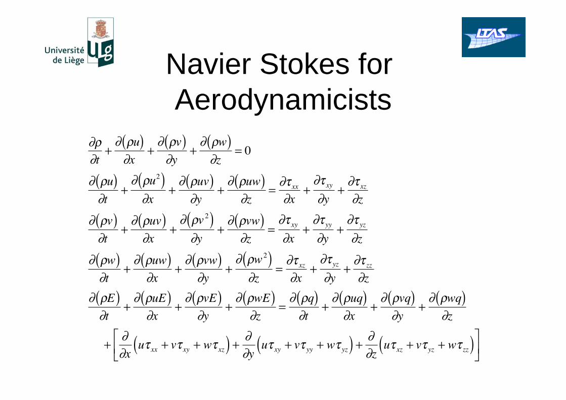
Navier Stokes for

Aerodynamicists

t+

u( )x

+v( )y

+w( )z

= 0

u( )t

+u2( )x

+uv( )y

+uw( )z

= xx

x+

xy

y+

xz

z

v( )t

+uv( )x

+v 2( )y

+vw( )z

=xy

x+

yy

y+

yz

z

w( )t

+uw( )x

+vw( )y

+w2( )z

=xz

x+

yz

y+

zz

z

E( )t

+uE( )x

+vE( )y

+wE( )z

=q( )t

+uq( )x

+vq( )y

+wq( )z

+xu xx + v xy + w xz( ) +

yu xy + v yy + w yz( ) +

zu xz + v yz + w zz( )

Nomenclature

• The lengths x, y, z are used to define position with respect to a global frame of reference, while time is defined by t.

• u, v, w are the local airspeeds. They are functions of position and time.

• p, , are the pressure, density and viscosity of the fluid and they are functions of position and time

• E is the total energy in the flow.

• q is the external heat flux

The stress tensor • Consider a small fluid element.

• In a general flow, each face of the element experiences normal stresses and shear stresses

• The three normal and six shear stress components make up the stress tensor

More nomenclature

• The components of the stress tensor:

• The total energy E is given by:

• where e is the internal energy of the flow

and depends on the temperature and

volume.

xx = p + 2μu

x, yy = p + 2μ

v

y, zz = p + 2μ

w

z

xy = yx = μv

x+

u

y

, yz = zy = μ

w

y+

v

z

, zx = xz = μ

u

z+

w

x

E = e +1

2u2 + v 2 + w2( )

Gas properties

• Do not forget that gases are also

governed by the state equation:

• Where T is the temperature and R is

Blotzmann’s constant.

• For a calorically perfect gas: e=cvT,

where cv is the specific heat at constant

volume.

p = RT

Comments on Navier-Stokes

equations • Notice that aerodynamicists always include the

mass and energy equations in the Navier-Stokes equations

• Notice also that compressibility is always allowed for, unless specifically ignored

• This is the most complete form of the airflow equations, although turbulence has not been explicitly defined

• Explicit definition of turbulence further complicates the equations by introducing new unknowns, the Reynolds stresses.

Constant viscosity

• Under the assumption that the fluid has

constant viscosity, the momentum

equations can be written as

u( )t

+u2( )x

+uv( )y

+uw( )z

=p

x+ μ

2u

x 2+

2u

y 2+

2u

z2

v( )t

+uv( )x

+v 2( )y

+vw( )z

=p

y+ μ

2v

x 2+

2v

y 2+

2v

z2

w( )t

+uw( )x

+vw( )y

+w2( )z

=p

z+ μ

2w

x 2+

2w

y 2+

2w

z2

Compact expressions

• There are several compact expressions

for the Navier-Stokes equations:

DuiDt

=p

xi+ μ

2uixi2Tensor notation:

Vector notation: ut

+1

2u u + u( ) u

= p + μ 2u

Matrix notation: ut

+TuuT

= p + μ 2Tu

Non-dimensional form

• The momentum equations can also be

written in non-dimensional form as

• where

u( )t

+u2( )x

+uv( )y

+uw( )z

=p

x+1Re

2u

x 2+

2u

y 2+

2u

z2

v( )t

+uv( )x

+v 2( )y

+vw( )z

=p

y+1

Re

2v

x 2+

2v

y 2+

2v

z2

w( )t

+uw( )x

+vw( )y

+w2( )z

=p

z+1Re

2w

x 2+

2w

y 2+

2w

z2

= , u =u

U, v =

v

U, w =

w

U, x =

x

L, y =

y

L, z =

z

L, t =

tL

U, p =

p

U 2

Solvability of the Navier-

Stokes equations

• There exist no solutions of the complete

Navier-Stokes equations

• The equations are:

– Unsteady

– Nonlinear

– Viscous

– Compressible

• The major problem is the nonlinearity

Flow unsteadiness

• Flow unsteadiness in the real world arises from two possible phenomena:

– The solid body accelerates

– There are areas of separated flows

• This course will only consider solid bodies that do not accelerate

• Attached flows will generally be considered

• Therefore, unsteady terms will be neglected

– All time derivatives in the Navier-Stokes equations are equal to zero

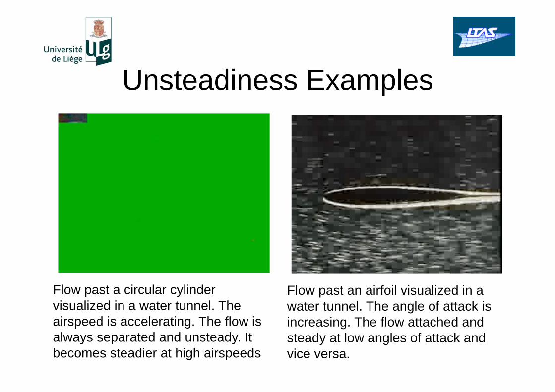
Unsteadiness Examples

Flow past a circular cylinder

visualized in a water tunnel. The

airspeed is accelerating. The flow is

always separated and unsteady. It

becomes steadier at high airspeeds

Flow past an airfoil visualized in a

water tunnel. The angle of attack is

increasing. The flow attached and

steady at low angles of attack and

vice versa.

Viscosity

• Viscosity is a property of fluids

• All fluids are viscous to different

degrees

• However, there are some aerodynamic

flow cases where viscosity can be

modeled in a simplified manner

• In those cases, all viscous terms are

neglected.

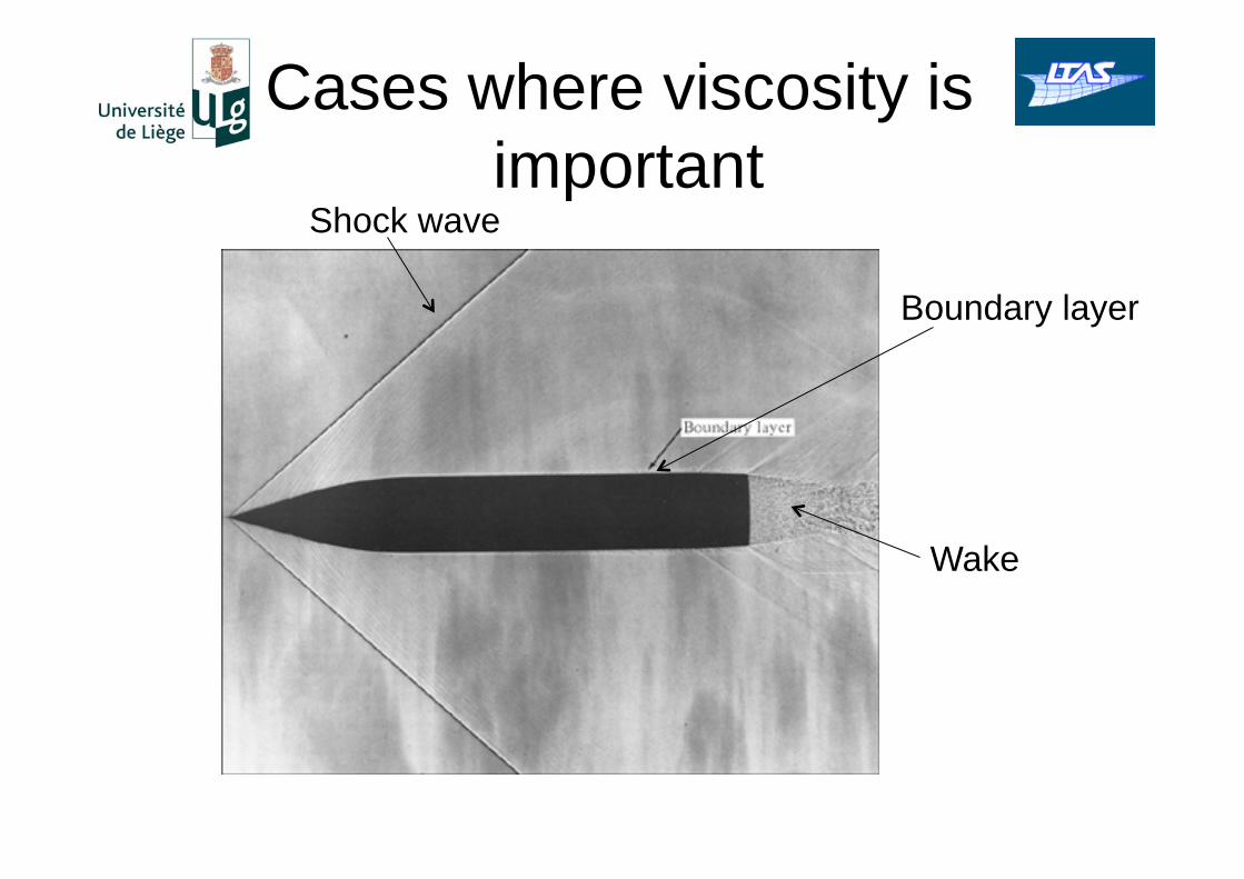
Cases where viscosity is

important

Wake

Shock wave

Boundary layer

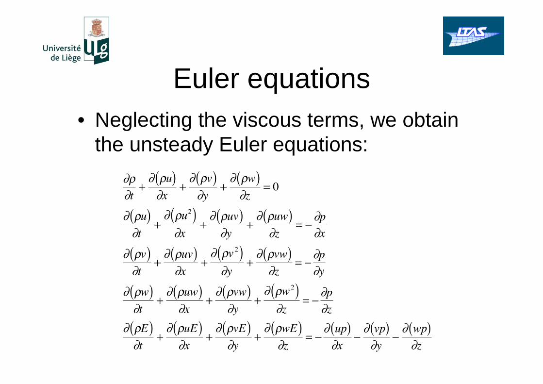
Euler equations

• Neglecting the viscous terms, we obtain

the unsteady Euler equations:

t+

u( )x

+v( )y

+w( )z

= 0

u( )t

+u2( )x

+uv( )y

+uw( )z

=p

x

v( )t

+uv( )x

+v 2( )y

+vw( )z

=p

y

w( )t

+uw( )x

+vw( )y

+w2( )z

=p

z

E( )t

+uE( )x

+vE( )y

+wE( )z

=up( )x

vp( )y

wp( )z

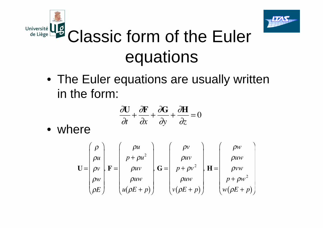
Classic form of the Euler

equations

• The Euler equations are usually written

in the form:

• where

Ut+Fx+Gy+Hz= 0

U =

u

v

w

E

, F =

u

p + u2

uv

uw

u E + p( )

, G =

v

uv

p + v 2

uw

v E + p( )

, H =

w

uw

vw

p + w2

w E + p( )

Steady Euler Equations

• Neglecting unsteady terms we obtain

the steady Euler equations:

u( )

x+

v( )

y+

w( )

z= 0

u2( )x

+uv( )

y+

uw( )

z=

p

x

uv( )

x+

v 2( )y

+vw( )

z=

p

y

uw( )

x+

vw( )

y+

w2( )z

=p

z

Example 1

• Notice that in the steady Euler

equations, the energy equation has

disappeared.

• Show that neglecting unsteady and

viscous terms turns the energy equation

into an identity if the air’s internal

energy is constant in space.

Compressibility

• The compressibility of most liquids is negligible for the forces encountered in engineering applications.

• Many fluid dynamicists always write the Navier-Stokes equations in incompressible form.

• This cannot be done for gases, as they are very compressible.

• However, for low enough airspeeds, the compressibility of gases also becomes negligible.

• In this case, compressibility can be ignored.

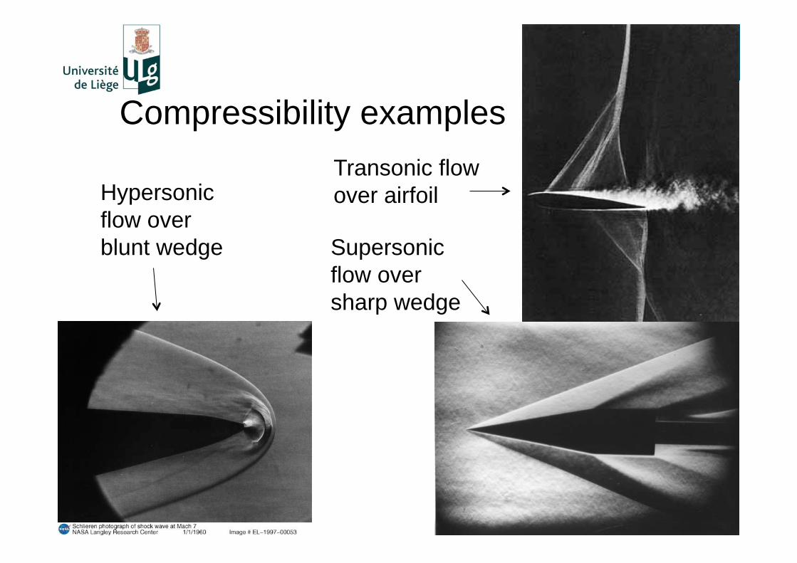
Compressibility examples

Transonic flow

over airfoil

Supersonic

flow over

sharp wedge

Hypersonic

flow over

blunt wedge

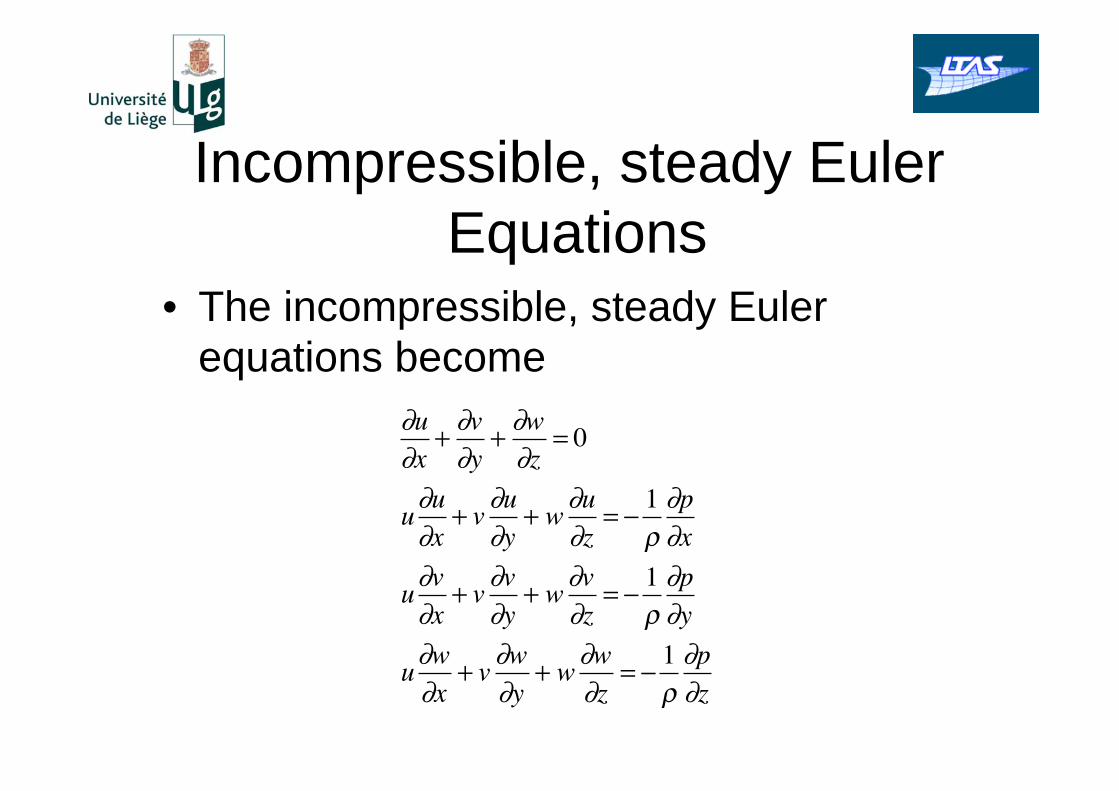
Incompressible, steady Euler

Equations • The incompressible, steady Euler

equations become

u

x+

v

y+

w

z= 0

uu

x+ v

u

y+ w

u

z=

1 p

x

uv

x+ v

v

y+ w

v

z=

1 p

y

uw

x+ v

w

y+ w

w

z=

1 p

z

Comment on the Euler

equations • The Euler equations are much more

solvable than the Navier-Stokes equations

• They are most commonly solved using numerical methods, such as finite differences

• There are very few analytical solutions of the Euler equations and they are not particularly useful

• In order to obtain analytical solutions, the equations must be simplified even further

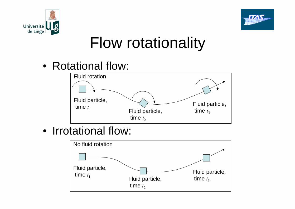
Flow rotationality

• Rotational flow:

• Irrotational flow:

Fluid particle,

time t1

Fluid rotation

Fluid particle,

time t2

Fluid particle,

time t3

Fluid particle,

time t1

No fluid rotation

Fluid particle,

time t2

Fluid particle,

time t3

Irrotationality (1)

• Some flows can be idealized as

irrotational

• In general, attached, incompressible,

inviscid flows are also irrotational

• Irrotationality requires that the curl of

the local velocity vector vanishes:

• where u=ui+vj+wk and

u = 0

=xi +

yj+

zk

Irrotationality (2)

• This leads to the simultaneous

equations:

• Integrating the momentum equations

using these conditions leads to the well-

known Bernoulli equation

w

y

v

z= 0,

w

x

u

z= 0,

v

x

u

y= 0

1

2u2 + v 2 + w2( ) + P = constant

Example 2

• Integrate the incompressible, steady

momentum equations to obtain

Bernoulli’s equation for irrotational flow

• You can start with the 2D equations

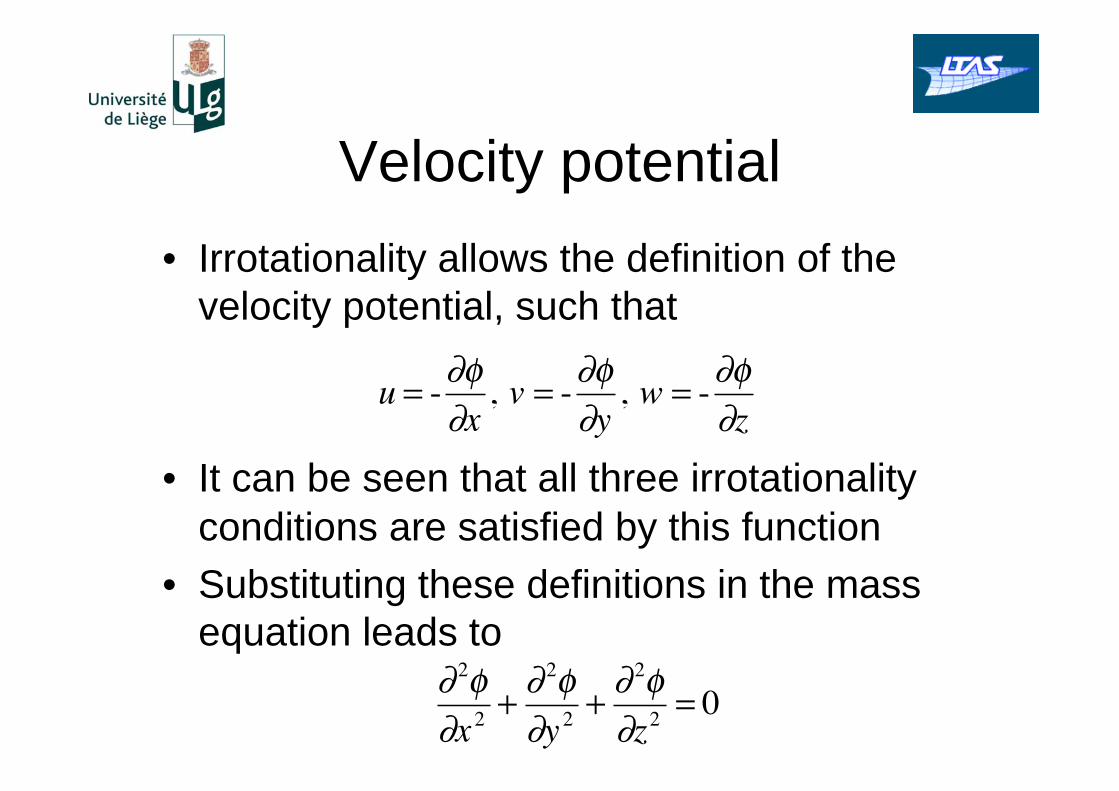
Velocity potential

• Irrotationality allows the definition of the

velocity potential, such that

• It can be seen that all three irrotationality

conditions are satisfied by this function

• Substituting these definitions in the mass

equation leads to

u = -x

, v = -y

, w = -z

2

x 2+

2

y 2+

2

z2= 0

Laplace’s equation

• The irrotational form of the Euler equations is Laplace’s equation.

• This is an equation that has many analytical solutions.

• It is the basis of most subsonic, attached flow aerodynamic assumptions.

• The equation is linear, therefore its solutions can be superimposed

• The complete flow problem has been reduced to a single, linear partial differential equation with a single unknown, the velocity potential.

Potential flow

• Incompressible, inviscid and irrotational flow is also called potential flow because it is fully described by the velocity potential.

• The first part of this course will look at potential flow solutions:

– First in two dimensions

– Then in three dimensions

• Potential flow solutions have provided us with the most useful and trustworthy aerodynamic results we have to date.

• Their limitations must be kept in mind at all times.

Potential flow solutions

• We now have a basis for modelling the

flow over 2D or 3D bodies. All we need

to do is:

– Solve Laplace’s equation

– With two boundary conditions (2nd order

problem):

• Impermeability: Flow cannot enter or exit a

solid body

• Far field: The flow far from the body is

undisturbed.

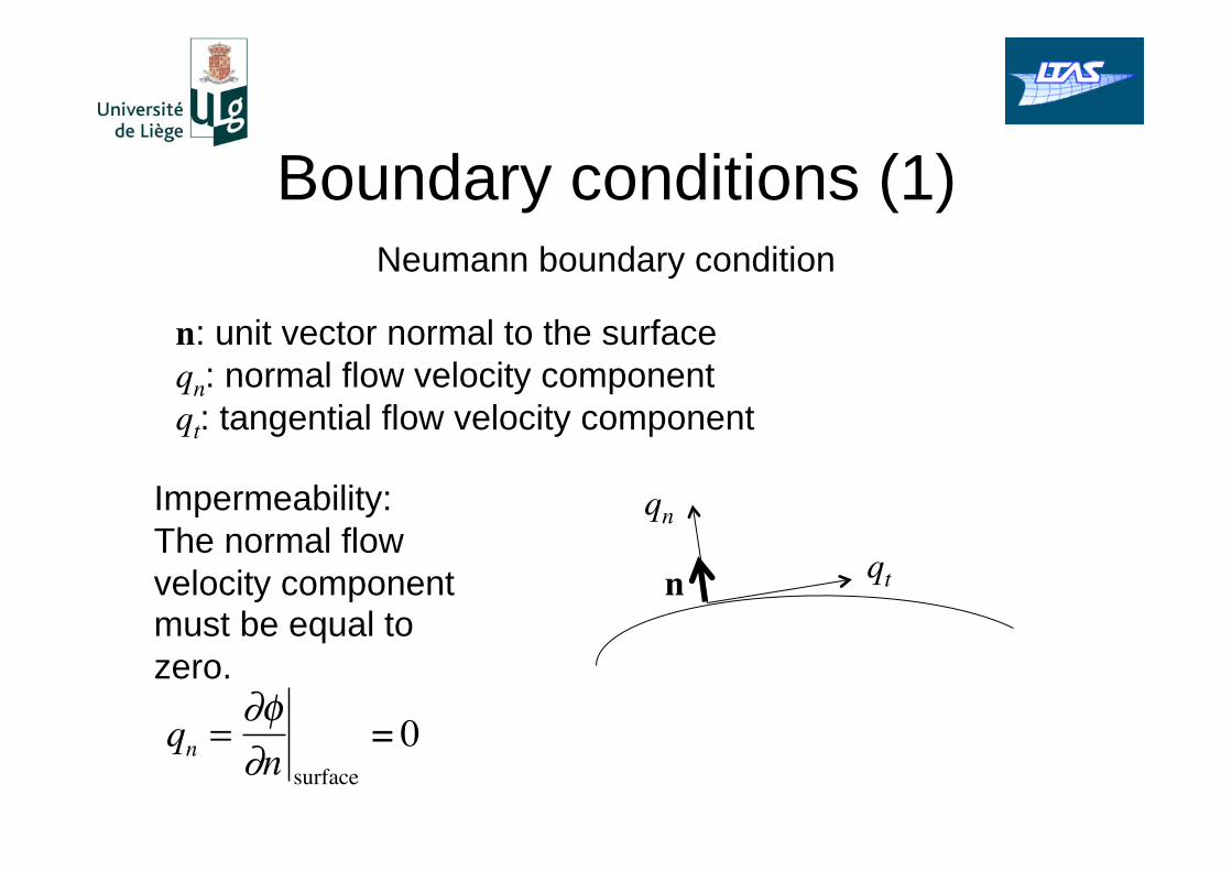
Boundary conditions (1)

qn

qt

Impermeability:

The normal flow

velocity component must be equal to

zero.

qn = n surface

= 0

n

n: unit vector normal to the surface

qn: normal flow velocity component

qt: tangential flow velocity component

Neumann boundary condition

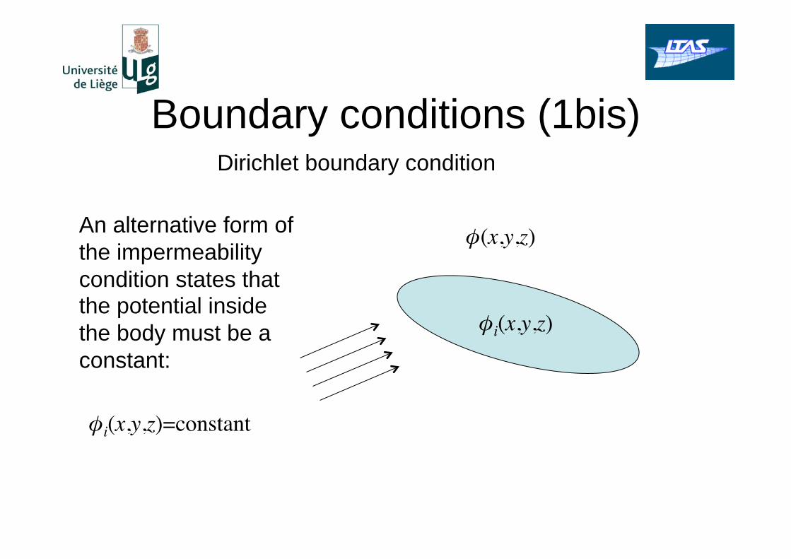
Boundary conditions (1bis)

(x,y,z)

i(x,y,z)

An alternative form of

the impermeability

condition states that the potential inside

the body must be a

constant:

i(x,y,z)=constant

Dirichlet boundary condition

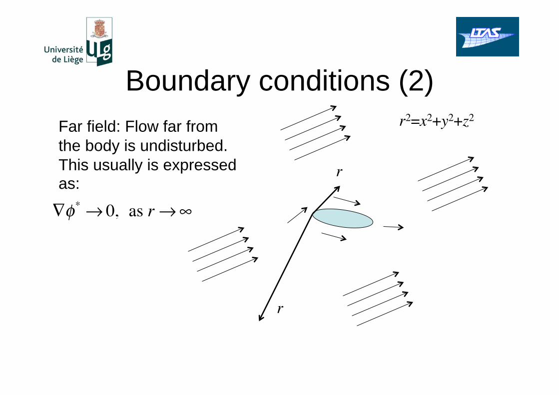
Boundary conditions (2)

Far field: Flow far from

the body is undisturbed.

This usually is expressed as:

* 0, as r

r

r

r2=x2+y2+z2

2D Potential Flow

• Two-dimensional flows don’t exist in reality but they are a useful simplification

• Two-dimensionality implies that the body being investigated: – Has an infinite span

– Does not vary geometrically with spanwise position

• As examples, consider an infinitely long circular cylinder or an infinitely long rectangular wing

2D Potential equations

• Laplace’s equation in two dimensions is

simply

• While the irrotationality condition is

• We still need to find solutions to this

equation.

2

x 2+

2

y 2= 0

v

x

u

y= 0

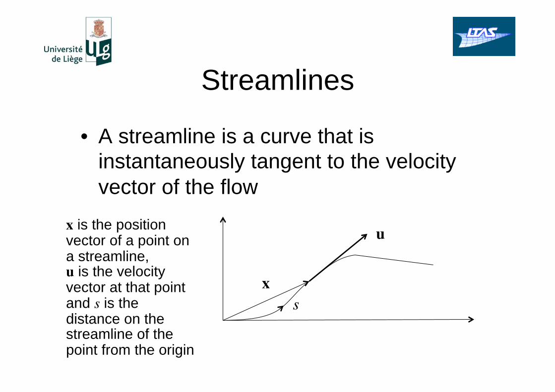
Streamlines

• A streamline is a curve that is

instantaneously tangent to the velocity

vector of the flow

u

xs

x is the position vector of a point on a streamline, u is the velocity vector at that point and s is the distance on the streamline of the point from the origin

Streamline definition

• A streamline is defined mathematically

as:

• Where u has components u, v, w and x has components x, y, z.

• It can be easily seen that the definition

leads to:

dxds

= u

dx

ds= u,

dy

ds= v,

dz

ds= w, and therefore

dx

u=

dy

v=

dz

w

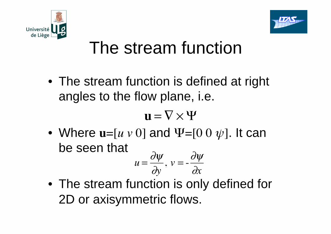
The stream function

• The stream function is defined at right

angles to the flow plane, i.e.

• Where u=[u v 0] and =[0 0 ]. It can

be seen that

• The stream function is only defined for

2D or axisymmetric flows.

u =

u =y

, v = -x

Properties of the stream

function

• The stream function automatically

satisfies the continuity equation.

• The stream is constant on a flow

streamline

• But, on a streamline

• Therefore

u

x+

v

y=

x y

+

y x

=

2

x y

2

x y= 0

d =xdx +

ydy = vdx + udy

dx

u=dy

v

d = udy + udy = 0

Elementary solutions

• There are several elementary solutions

of Laplace’s equation:

– The free stream: rectilinear motion of the

airflow

– The source: a singularity that creates a

radial velocity field around it

– The sink: the opposite of a source

– The doublet: a combined source and sink

– The vortex: a singularity that creates a

circular velocity field around it.

Historical perspective

• 1738: Daniel Bernoulli developed Bernoulli’s principle, which leads to Bernoulli’s equation.

• 1740: Jean le Rond d'Alembert studied inviscid, incompressible flow and formulated his paradox.

• 1755: Leonhard Euler derived the Euler equations.

• 1743: Alexis Clairaut first suggested the idea of a scalar potential.

• 1783: Pierre-Simon Laplace generalized the idea of the scalar potential and showed that all potential functions satisfy the same equation: Laplace’s equation.

• 1822: Louis Marie Henri Navier first derived the Navier-Stokes equations from a molecular standpoint.

• 1828: Augustin Louis Cauchy also derived the Navier-Stokes equations

• 1829: Siméon Denis Poisson also derived the Navier-Stokes equations

• 1843: Adhémar Jean Claude Barré de Saint-Venant derived the Navier-Stokes equations for both laminar and turbulent flow. He also was the first to realize the importance of the coefficient of viscosity.

• 1845: George Gabriel Stokes published one more derivation of the Navier-Stokes equations.