Lecture 1Introduction to R

Andrew Jaffe

Instructor

Welcome to class!1. Introductions

2. Class overview

3. Getting R up and running

4. File Input/Output

2/77

About MePostdoctoral Fellow at the Lieber Institute for Brain Development

PhD in Epidemiology, MHS in Bioinformatics

Email: andrewejaffe@gmail.com

3/77

TAJohn Muschelli

PhD Student in Biostatistics

Email: muschellij2@gmail.com

4/77

IntroductionsWhat do you hope to get out of the class?

Why R?

5/77

Course Websitehttp://biostat.jhsph.edu/~ajaffe/rwinter2013.html

Materials will be uploaded the night before class

6/77

Learning ObjectivesReading data into R

Recoding and manipulating data

Writing R functions and using add-on packages

Making exploratory plots

Performing basic statistical tests

Understanding basic programming syntax

·

·

·

·

·

·

7/77

Course Format1. 90 minute interactive lectures

2. 5-10 minute break

3. Lab

HTML Slides

Pausing to interact with R

·

·

90 minutes: working on exercises in small groups

10-15 minutes: coming back together to discuss

·

·

8/77

Grading1. Attendance/Participation: 20%

2. Nightly "Homework": 3 x 15%

3. Final "Project": 35%

Individual: extension of each lab

Turn In: Correct Answers + R Code

·

·

9/77

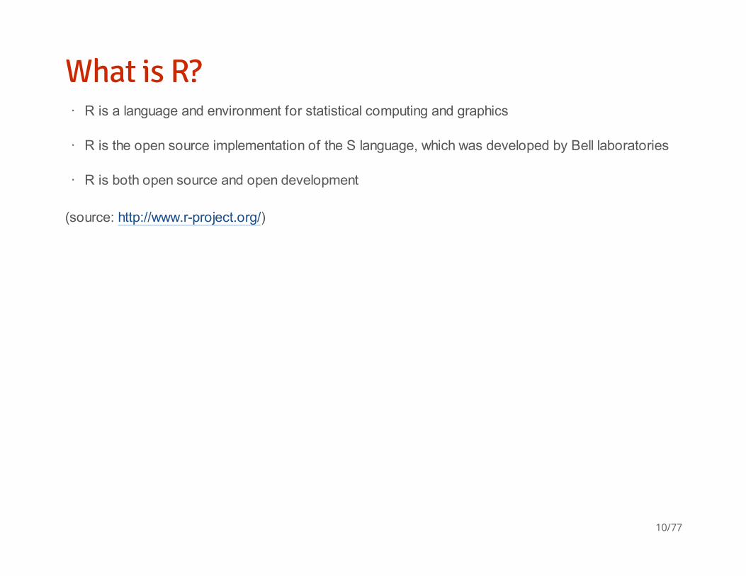
What is R?

(source: http://www.r-project.org/)

R is a language and environment for statistical computing and graphics

R is the open source implementation of the S language, which was developed by Bell laboratories

R is both open source and open development

·

·

·

10/77

Why R?Powerful and flexible

Free (open source)

Extensive add-on software

Designed for statistical computing

High level language

·

·

·

·

·

11/77

Why not R?Fairly steep learning curve

Little centralized support, relies on online community and package developers

Annoying to update

Slower, and more memory intensive, than the more traditional programming languages (C, Java,

Perl, Python)

·

"Programming" oriented

Minimal interface

-

-

·

·

·

12/77

Installing RInstall the latest version from: http://cran.r-project.org/

Note that you must manually update R, often at your own peril...

13/77

R StudioIntegrated Development Environment (IDE) for R

http://www.rstudio.com/

·

Syntax highlighting, code completion, and smart indentation

Execute R code directly from the source editor

Easily manage multiple working directories using projects

Workspace browser and data viewer

Plot history, zooming, and flexible image and PDF export

Integrated R help and documentation

Searchable command history

-

-

-

-

-

-

-

·

14/77

15/77

Working with RThe R Console "interprets" whatever you type

"Analysis" Script + Interactive Exploration

R revolves around 'functions'

·

Calculator

Creating variables

Applying functions

-

-

-

·

Static copy of what you did

Try things out interactively, then add to your script

-

-

·

Commands that take input, performs computations, and returns results

Many come with R, but people write external functions you can download and use

-

-

16/77

Getting StartedYou should have the latest version of R installed (R 2.15.2 as of 12/31/12)!

Open R Studio

Files --> New --> R Script

Save the blank R script as "lecture1.R" in a directory of your choosing

Add a comment header

·

·

·

·

·

17/77

Commenting in ScriptsAdd a comment header to lecture1.R : '#' is the comment symbol

################## Title: Demo R Script# Author: Andrew Jaffe# Date: 1/7/2013# Purpose: Demonstrate comments in R###################

# this is a comment, nothing to the right of it gets read

# this # is still a comment - you can use many #'s as you want

# sometimes you have a really long comment, like explaining what you # are doing for a step in analysis. Take it to a second line

18/77

Useful R Studio Shortcuts'Ctrl+1' takes you to the script page

'Ctrl+2' takes you to the console

'Ctrl + Enter' ('Cmd + Enter' on OS X) in your script evaluates that line of code

·

·

·

19/77

FunctionsR revolves around functions: denoted by "()"

Every function takes an input, defined by arguments, often provided by the user

Many functions have default settings for these arguments

If you know the name of a function, "?[function name]" or 'help([function name])' will pop up the help

menu

'example([function name])' shows you how it is used

·

·

·

·

·

20/77

Working DirectoryR looks for files on your computer relative to the "working" directory

It's always safer to set the working directory at the beginning of your script

Example of help file

·

·

·

> ## get the working directory> getwd()

[1] "C:/Users/Andrew/Dropbox/WinterRClass/Lectures/lecture1"

> ### set the working directory> ### setwd('F:/Hopkins/Lieber/Classes/WinterInstituteR/Lectures') # desktop> setwd("..")> getwd()

[1] "C:/Users/Andrew/Dropbox/WinterRClass/Lectures"

21/77

Working DirectorySetting the directory can sometimes be finicky

Regular directory structure shortcuts apply

·

Windows: Default directory structure involves single backslashes ("\"), but R interprets these as

"escape" characters. So you must replace the backslash with forward slashed ("/") or two

backslashes ("\")

Mac/Linux: Default is forward slashes, so you are okay

-

-

·

".." goes up one level

"./" is the current directory

"~" is your home directory

-

-

-

22/77

Working DirectoryTry some directory navigation:

> dir("./") # shows directory contents

[1] "assets" "index.html" "index.md" [4] "index.Rmd" "Lecture 1.pdf" "lecture1_code.R" [7] "lecture1_test.html" "libraries" "Monuments.csv" [10] "pics"

> dir("..")

[1] "extra code" "extra_code.R" "lecture1" "lecture2" [5] "lecture3" "lecture4" "lecture5"

> head(dir("F:/Hopkins/Lieber"))

[1] "Classes" "Documents" [3] "jaffe-website bio.docx" "Jobs" [5] "Research"

23/77

Working DirectorySet your working directory to the same location where you saved the blank R script: "lecture1.R"

Confirm the directory contains "lecture1.R"

·

·

24/77

R as a calculator> 2 + 2

[1] 4

> 2 * 4

[1] 8

> 2̂3

[1] 8

25/77

R as a calculatorThe R console is a full calculator

Try to play around with it:

·

·

+, -, /, * are add, subtract, multiply, and divide

^ or ** is power

( and ) work with order of operations

-

-

-

26/77

R as a calculator> 2 + (2 * 3)̂2

[1] 38

> (1 + 3)/2 + 45

[1] 47

27/77

R variablesYou can create variables from within the R environment and from files on your computer

R uses "=" or "<-" to assign values to a variable name

Variable names are case-sensitive, i.e. X and x are different

·

·

·

> x = 2> x

[1] 2

> x * 4

[1] 8

> x + 2

[1] 4

28/77

R variablesEach variable has a 'class' associated with it·

> class(x)

[1] "numeric"

> y = "hello world!"> print(y)

[1] "hello world!"

> class(y)

[1] "character"

29/77

R variablesYou can get more attributes than just class·

> ## ?str> str(x)

num 2

> str(y)

chr "hello world!"

30/77

The 'combine' functionThe function 'c()' collects/combines/joins single R objects into a vector of R objects. It is mostly used

for creating vectors of numbers, character strings, and other data types.

> x <- c(1, 4, 6, 8)> x

[1] 1 4 6 8

> str(x)

num [1:4] 1 4 6 8

31/77

R variableslength(): Get or set the length of vectors (including lists) and factors, and of any other R object for

which a method has been defined.

> length(x)

[1] 4

> y

[1] "hello world!"

> length(y)

[1] 1

32/77

R variables> x + 2

[1] 3 6 8 10

> x * 3

[1] 3 12 18 24

> x + c(1, 2, 3, 4)

[1] 2 6 9 12

33/77

R variables

Note that the R object 'y' is no longer "Hello World!" - It has effectively been overwritten by assigning

new data to the variable

> y = x + c(1, 2, 3, 4)> y

[1] 2 6 9 12

34/77

ReviewCreating a new script

Using R as a calculator

Assigning values to variables

Performing algebra on numeric variables

·

·

·

·

35/77

Data Input'Reading in' data is the first step of any project/analysis

R can read almost any file format, especially via add-on packages

We are going to focus on simple delimited files first

There are also pre-installed sample datasets in R that we might use in class

·

·

·

tab delimited (e.g. '.txt')

comma separated (e.g. '.csv')

Microsoft excel (e.g. '.xlsx')

-

-

-

·

36/77

Data Inputread.table(): Reads a file in table format and creates a data frame from it, with cases corresponding to

lines and variables to fields in the file.

# the four ones I've put at the top are the important inputsread.table( file, # filename header = FALSE, # are there column names? sep = "", # what separates columns? as.is = !stringsAsFactors, # do you want character strings as factors or characters? quote = "\"'", dec = ".", row.names, col.names, na.strings = "NA", nrows = -1, skip = 0, check.names = TRUE, fill = !blank.lines.skip, strip.white = FALSE, blank.lines.skip = TRUE, comment.char = "#", stringsAsFactors = default.stringsAsFactors())

# for example: read.table("file.txt", header = TRUE, sep="\t", as.is=TRUE)

37/77

Data InputThe filename is the path to your file, in quotes

The function will look in your working directory if no absolute path is given

The same back- and forward-slash rules apply as setting the working directory

Note that the filename can also be a path to a file on a website (e.g. 'www.someurl.com/table1.txt')

·

·

·

·

38/77

Data AsideEverything we do in class will be using real publicly available data - there are no 'toy' example

datasets or 'simulated' data

OpenBaltimore and Data.gov will be sources for the first few days

·

·

39/77

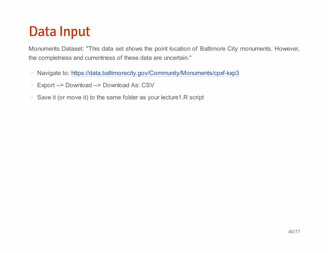
Data InputMonuments Dataset: "This data set shows the point location of Baltimore City monuments. However,

the completness and currentness of these data are uncertain."

Navigate to: https://data.baltimorecity.gov/Community/Monuments/cpxf-kxp3

Export --> Download --> Download As: CSV

Save it (or move it) to the same folder as your lecture1.R script

·

·

·

40/77

Data InputThere is a 'wrapper' function for reading CSV files:

Note: the '...' designates arguments that are passed to read.table()

read.csv

## function (file, header = TRUE, sep = ",", quote = "\"", dec = ".", ## fill = TRUE, comment.char = "", ...) ## read.table(file = file, header = header, sep = sep, quote = quote, ## dec = dec, fill = fill, comment.char = comment.char, ...)## <bytecode: 0x000000000dbeefd0>## <environment: namespace:utils>

41/77

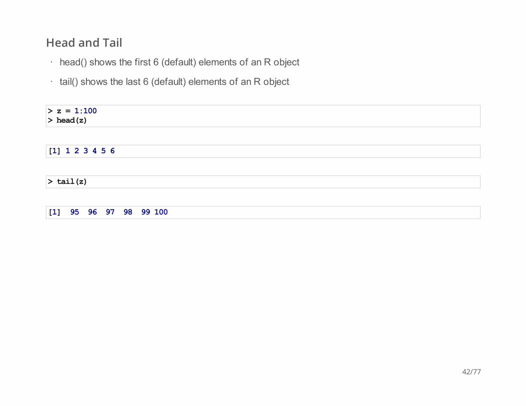
Head and Tail

head() shows the first 6 (default) elements of an R object

tail() shows the last 6 (default) elements of an R object

·

·

> z = 1:100> head(z)

[1] 1 2 3 4 5 6

> tail(z)

[1] 95 96 97 98 99 100

42/77

Data Inputmon = read.csv("Monuments.csv", header = TRUE, as.is = TRUE)head(mon)

name zipCode neighborhood councilDistrict1 James Cardinal Gibbons 21201 Downtown 112 The Battle Monument 21202 Downtown 113 Negro Heroes of the U.S Monument 21202 Downtown 114 Star Bangled Banner 21202 Downtown 115 Flame at the Holocaust Monument 21202 Downtown 116 Calvert Statue 21202 Downtown 11 policeDistrict Location.11 CENTRAL 408 CHARLES ST\nBaltimore, MD\n2 CENTRAL 3 CENTRAL 4 CENTRAL 100 HOLLIDAY ST\nBaltimore, MD\n5 CENTRAL 50 MARKET PL\nBaltimore, MD\n6 CENTRAL 100 CALVERT ST\nBaltimore, MD\n

43/77

Data InputThe read.table() function returns a 'data.frame'

> class(mon)

[1] "data.frame"

> str(mon)

'data.frame': 84 obs. of 6 variables: $ name : chr "James Cardinal Gibbons" "The Battle Monument" "Negro Heroes of the U.S Monument" $ zipCode : int 21201 21202 21202 21202 21202 21202 21202 21211 21213 21211 ... $ neighborhood : chr "Downtown" "Downtown" "Downtown" "Downtown" ... $ councilDistrict: int 11 11 11 11 11 11 11 7 14 14 ... $ policeDistrict : chr "CENTRAL" "CENTRAL" "CENTRAL" "CENTRAL" ... $ Location.1 : chr "408 CHARLES ST\nBaltimore, MD\n" "" "" "100 HOLLIDAY ST\nBaltimore, MD\n" ...

44/77

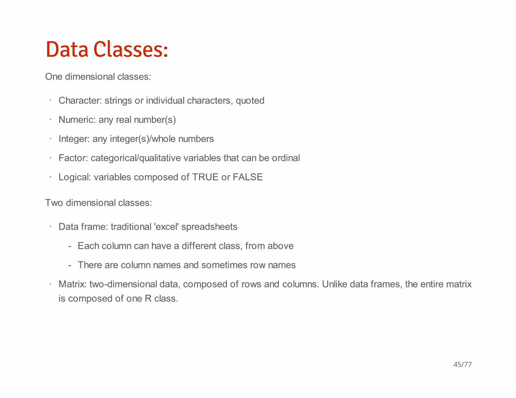
Data Classes:One dimensional classes:

Two dimensional classes:

Character: strings or individual characters, quoted

Numeric: any real number(s)

Integer: any integer(s)/whole numbers

Factor: categorical/qualitative variables that can be ordinal

Logical: variables composed of TRUE or FALSE

·

·

·

·

·

Data frame: traditional 'excel' spreadsheets

Matrix: two-dimensional data, composed of rows and columns. Unlike data frames, the entire matrix

is composed of one R class.

·

Each column can have a different class, from above

There are column names and sometimes row names

-

-

·

45/77

Matrices> n = 1:9 # sequence from first number to second number incrementing by 1> n

[1] 1 2 3 4 5 6 7 8 9

> mat = matrix(n, nr = 3)> mat

[,1] [,2] [,3][1,] 1 4 7[2,] 2 5 8[3,] 3 6 9

46/77

Matrix and Data frame Attributesnrow() displays the number of rows of a matrix or data frame

ncol() displays the number of coloumns

dim() displays a vector of length 2: # rows, # columns

colnames() displays the column names (if any) and rownames() displays the row names (if any)

·

·

·

·

47/77

Data SelectionBrackets are used to select and/or subset data in R

> x1 = 10:20> x1

[1] 10 11 12 13 14 15 16 17 18 19 20

> length(x1)

[1] 11

48/77

Data Selection> x1[1] # selecting first element

[1] 10

> x1[3:4] # selecting third and fourth elements

[1] 12 13

> x1[c(1, 5, 7)] # selecting first, fifth, and seventh elements

[1] 10 14 16

49/77

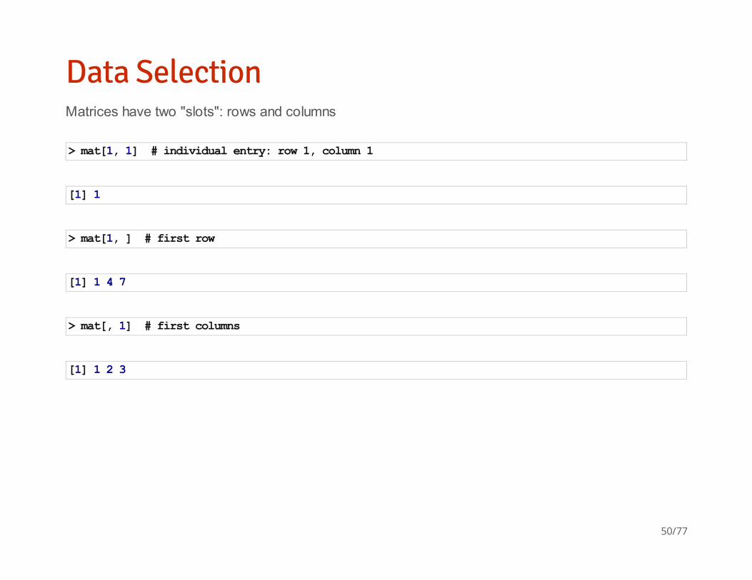
Data SelectionMatrices have two "slots": rows and columns

> mat[1, 1] # individual entry: row 1, column 1

[1] 1

> mat[1, ] # first row

[1] 1 4 7

> mat[, 1] # first columns

[1] 1 2 3

50/77

Data SelectionNote that the class of the returned object is no longer a matrix

> class(mat[1, ])

[1] "integer"

> class(mat[, 1])

[1] "integer"

51/77

Data SelectionData frames have special ways to select data, specifically by a "$" and the column name

> names(mon)

[1] "name" "zipCode" "neighborhood" "councilDistrict"[5] "policeDistrict" "Location.1"

> head(mon$zipCode)

[1] 21201 21202 21202 21202 21202 21202

> head(mon$neighborhood)

[1] "Downtown" "Downtown" "Downtown" "Downtown" "Downtown" "Downtown"

52/77

Data SelectionYou can also subset data frames like matrices, using row and column indices, but using column names

is generally safer and more reproducible.

You can also use the bracket notation, but specify the name(s) in quotes if you want more than 1

column. This allows you to subset rows and columns at the same time

> head(mon[, 2])

[1] 21201 21202 21202 21202 21202 21202

> mon[1:3, c("name", "zipCode")]

name zipCode1 James Cardinal Gibbons 212012 The Battle Monument 212023 Negro Heroes of the U.S Monument 21202

53/77

Unique entriesunique(): unique returns a vector, data frame or array like x but with duplicate elements/rows removed.

Note that this does NOT sort entries - it just returns the unique entries in the order it encounters them

from first to last:

> x = c(1, 2, 3, 4, 4, 5, 4, 5)> unique(x)

[1] 1 2 3 4 5

> unique(c(5, 1, 2, 3, 4, 4, 5, 4, 5))

[1] 5 1 2 3 4

54/77

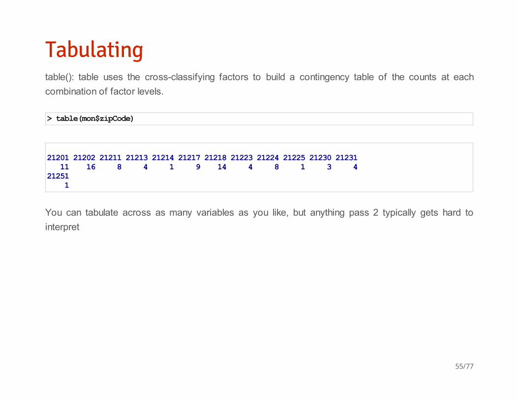
Tabulatingtable(): table uses the cross-classifying factors to build a contingency table of the counts at each

combination of factor levels.

You can tabulate across as many variables as you like, but anything pass 2 typically gets hard to

interpret

> table(mon$zipCode)

21201 21202 21211 21213 21214 21217 21218 21223 21224 21225 21230 21231 11 16 8 4 1 9 14 4 8 1 3 4 21251 1

55/77

Lab 1A: Explore 'Monument' DatasetSolve using your favorite method (R, Excel, By Eye/Counting Manually, etc):

1. Change the name of the "Location.1" column to "location"

2. How many monuments are in Baltimore (at least this collection...)?

3. What are the (a) zip codes, (b) neighborhoods, (c) council districts, and (d) police districts that

contain monuments, and how many monuments are in each?

4. How many zip codes are in the (a) "Downtown" and (b) "Johns Hopkins Homewood"

neighborhoods?

5. How many monuments (a) do and (b) do not have an exact location?

6. Which (a) zip code, (b) neighborhood, (c) council district, and (d) police district contains the most

number of monuments?

56/77

Question 1Names are just an attribute of the data frame (recall str) that you can change to any valid character

name

Valid character names are case-sensitive, contain a-z, 0-9, underscores, and periods (but cannot start

with a number).

For data frames, colnames() and names() return the same attribute.

These naming rules also apply for creating R objects

> names(mon)

[1] "name" "zipCode" "neighborhood" "councilDistrict"[5] "policeDistrict" "Location.1"

> names(mon)[6] = "location"> names(mon)

[1] "name" "zipCode" "neighborhood" "councilDistrict"[5] "policeDistrict" "location"

57/77

Question 2There are several ways to return the number of rows of a data frame or matrix

> nrow(mon)

[1] 84

> dim(mon)

[1] 84 6

> length(mon$name)

[1] 84

58/77

Question 3unique() returns the unique entries in a vector

> unique(mon$zipCode)

[1] 21201 21202 21211 21213 21217 21218 21224 21230 21231 21214 21223[12] 21225 21251

> unique(mon$policeDistrict)

[1] "CENTRAL" "NORTHERN" "NORTHEASTERN" "WESTERN" [5] "SOUTHEASTERN" "SOUTHERN" "EASTERN"

> unique(mon$councilDistrict)

[1] 11 7 14 13 1 10 3 2 9 12

59/77

> unique(mon$neighborhood)

[1] "Downtown" "Remington" [3] "Clifton Park" "Johns Hopkins Homewood" [5] "Mid-Town Belvedere" "Madison Park" [7] "Upton" "Reservoir Hill" [9] "Harlem Park" "Coldstream Homestead Montebello"[11] "Guilford" "McElderry Park" [13] "Patterson Park" "Canton" [15] "Middle Branch/Reedbird Parks" "Locust Point Industrial Area" [17] "Federal Hill" "Washington Hill" [19] "Inner Harbor" "Herring Run Park" [21] "Ednor Gardens-Lakeside" "Fells Point" [23] "Hopkins Bayview" "New Southwest/Mount Clare" [25] "Brooklyn" "Stadium Area" [27] "Mount Vernon" "Druid Hill Park" [29] "Morgan State University" "Dunbar-Broadway" [31] "Carrollton Ridge" "Union Square"

60/77

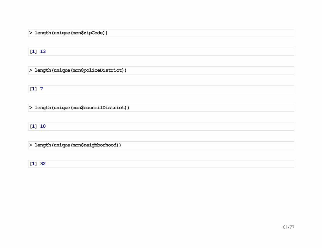
> length(unique(mon$zipCode))

[1] 13

> length(unique(mon$policeDistrict))

[1] 7

> length(unique(mon$councilDistrict))

[1] 10

> length(unique(mon$neighborhood))

[1] 32

61/77

Also note that table() can work, which tabulates a specific variable (or cross-tabulates two variables)

> table(mon$zipCode)

21201 21202 21211 21213 21214 21217 21218 21223 21224 21225 21230 21231 11 16 8 4 1 9 14 4 8 1 3 4 21251 1

> length(table(mon$zipCode))

[1] 13

62/77

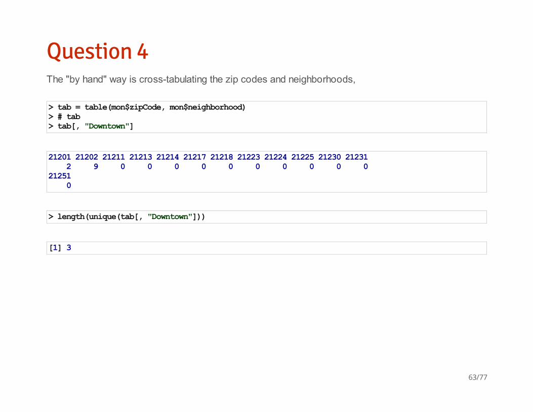
Question 4The "by hand" way is cross-tabulating the zip codes and neighborhoods,

> tab = table(mon$zipCode, mon$neighborhood)> # tab> tab[, "Downtown"]

21201 21202 21211 21213 21214 21217 21218 21223 21224 21225 21230 21231 2 9 0 0 0 0 0 0 0 0 0 0 21251 0

> length(unique(tab[, "Downtown"]))

[1] 3

63/77

Logical StatementsBut we want non-zero entries. This introduces the logical class, which consists of either TRUE or

FALSE

> z = c(TRUE, FALSE, TRUE, FALSE)> class(z)

[1] "logical"

> sum(z)

[1] 2

64/77

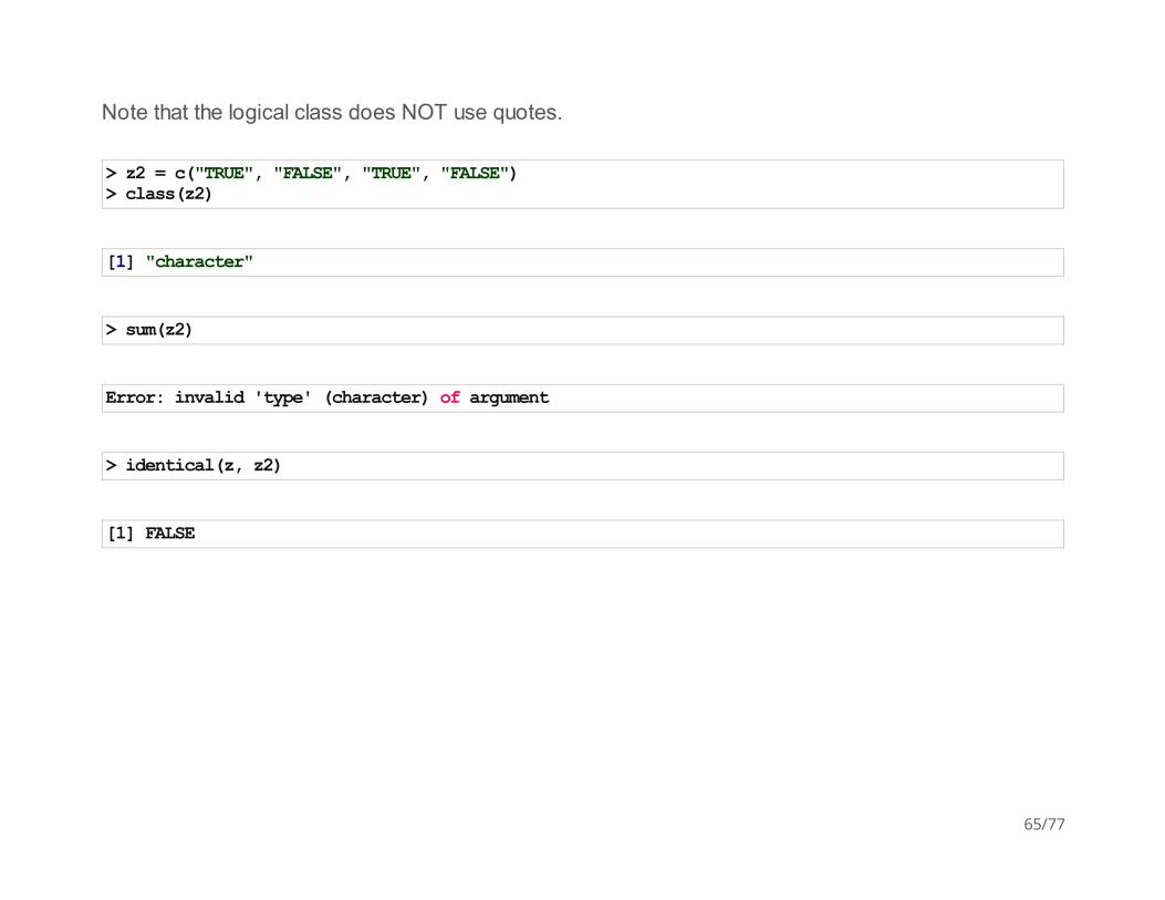
Note that the logical class does NOT use quotes.

> z2 = c("TRUE", "FALSE", "TRUE", "FALSE")> class(z2)

[1] "character"

> sum(z2)

Error: invalid 'type' (character) of argument

> identical(z, z2)

[1] FALSE

65/77

Logical StatementsThis mirrors computer science/programming syntax:·

'==': equal to

'!=': not equal to (it is NOT '~' in R, e.g. SAS)

'>': greater than

'<': less than

'>=': greater than or equal to

'<=': less than or equal to

-

-

-

-

-

-

66/77

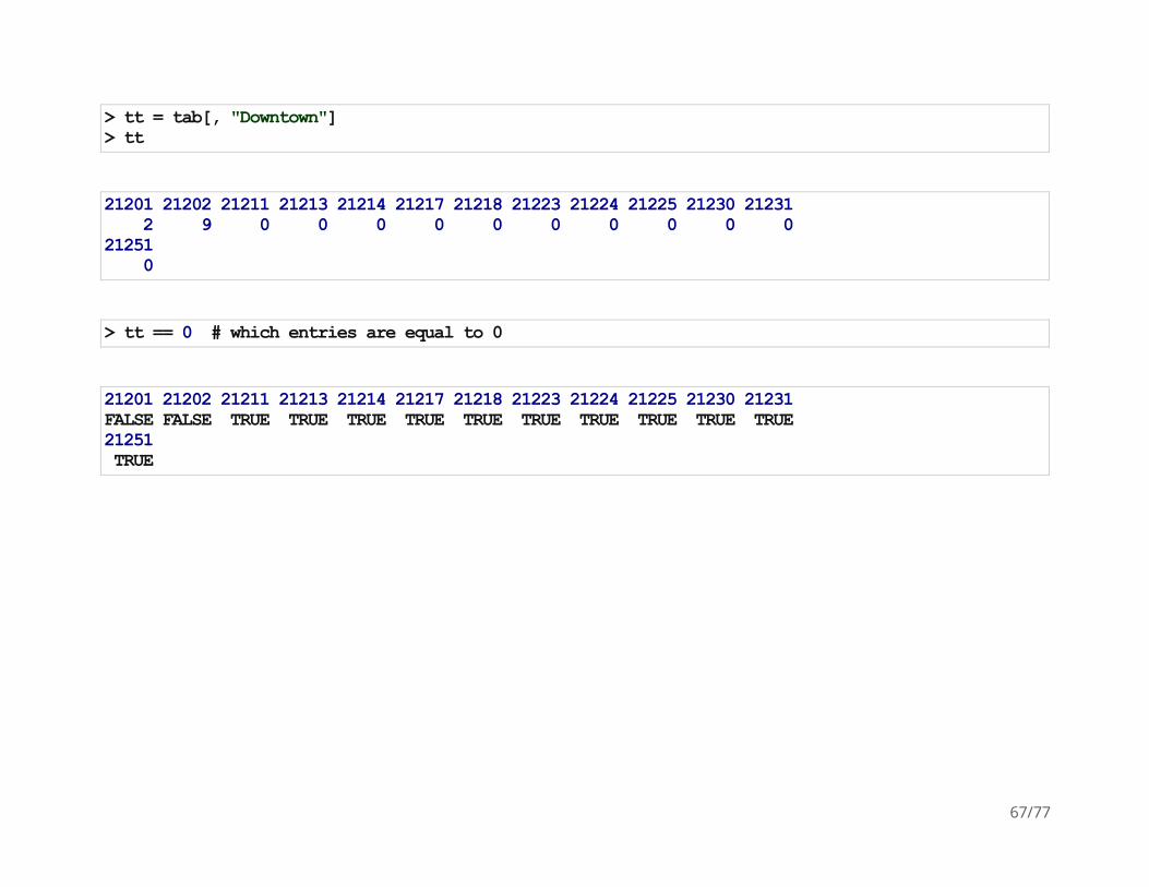
> tt = tab[, "Downtown"]> tt

21201 21202 21211 21213 21214 21217 21218 21223 21224 21225 21230 21231 2 9 0 0 0 0 0 0 0 0 0 0 21251 0

> tt == 0 # which entries are equal to 0

21201 21202 21211 21213 21214 21217 21218 21223 21224 21225 21230 21231 FALSE FALSE TRUE TRUE TRUE TRUE TRUE TRUE TRUE TRUE TRUE TRUE 21251 TRUE

67/77

> tab[, "Downtown"] != 0

21201 21202 21211 21213 21214 21217 21218 21223 21224 21225 21230 21231 TRUE TRUE FALSE FALSE FALSE FALSE FALSE FALSE FALSE FALSE FALSE FALSE 21251 FALSE

> sum(tab[, "Downtown"] != 0)

[1] 2

> sum(tab[, "Johns Hopkins Homewood"] != 0)

[1] 2

68/77

We could also subset the data into neighborhoods:

> dt = mon[mon$neighborhood == "Downtown", ]> head(mon$neighborhood == "Downtown", 10)

[1] TRUE TRUE TRUE TRUE TRUE TRUE TRUE FALSE FALSE FALSE

> dim(dt)

[1] 11 6

> length(unique(dt$zipCode))

[1] 2

69/77

Question 5> head(mon$location)

[1] "408 CHARLES ST\nBaltimore, MD\n" "" [3] "" "100 HOLLIDAY ST\nBaltimore, MD\n"[5] "50 MARKET PL\nBaltimore, MD\n" "100 CALVERT ST\nBaltimore, MD\n"

> table(mon$location != "") # FALSE=DO NOT and TRUE=DO

FALSE TRUE 26 58

70/77

Question 6> tabZ = table(mon$zipCode)> head(tabZ)

21201 21202 21211 21213 21214 21217 11 16 8 4 1 9

> max(tabZ)

[1] 16

> tabZ[tabZ == max(tabZ)]

21202 16

71/77

which.max() returns the FIRST entry/element number that contains the maximum and which.min()

returns the FIRST entry that contains the minimum

> which.max(tabZ) # this is the element number

21202 2

> tabZ[which.max(tabZ)] # this is the actual maximum

21202 16

72/77

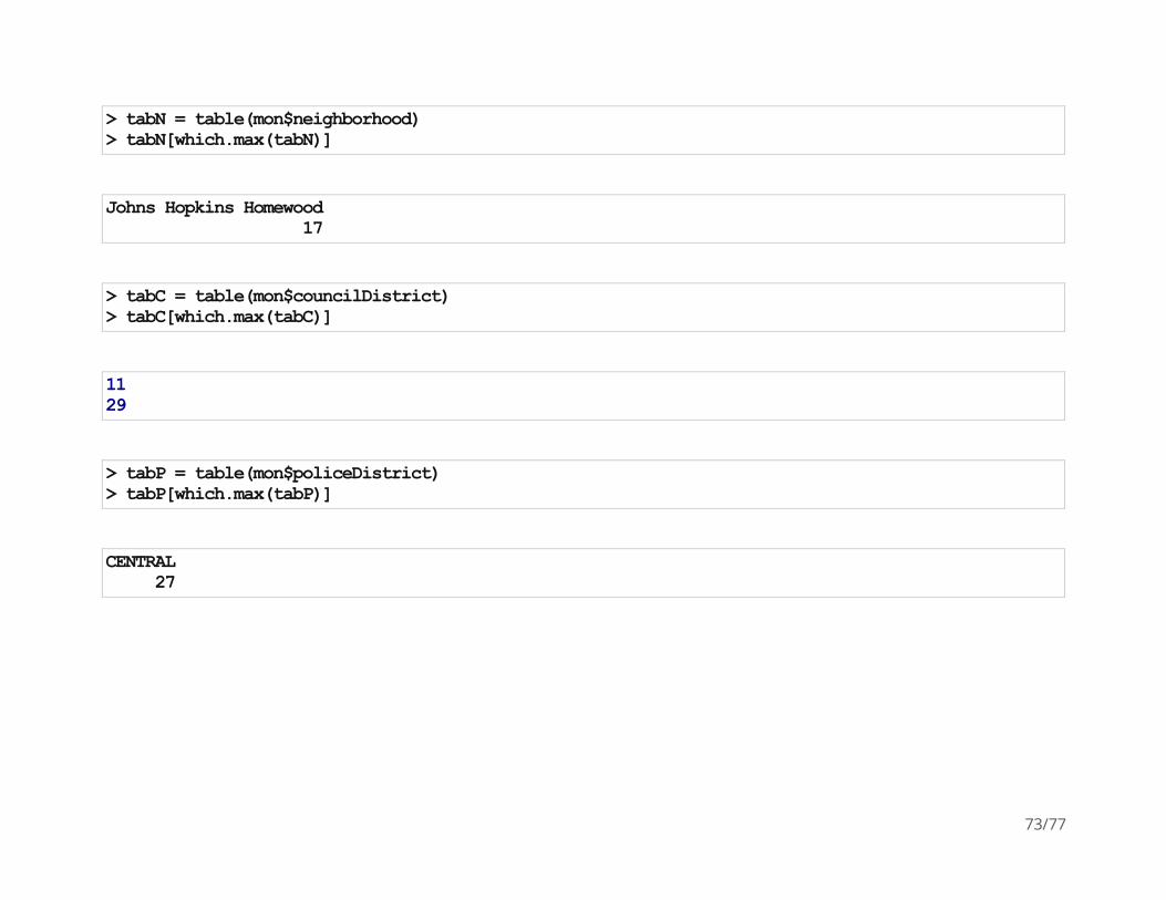
> tabN = table(mon$neighborhood)> tabN[which.max(tabN)]

Johns Hopkins Homewood 17

> tabC = table(mon$councilDistrict)> tabC[which.max(tabC)]

11 29

> tabP = table(mon$policeDistrict)> tabP[which.max(tabP)]

CENTRAL 27

73/77

Other Useful R Stuff to get you going

74/77

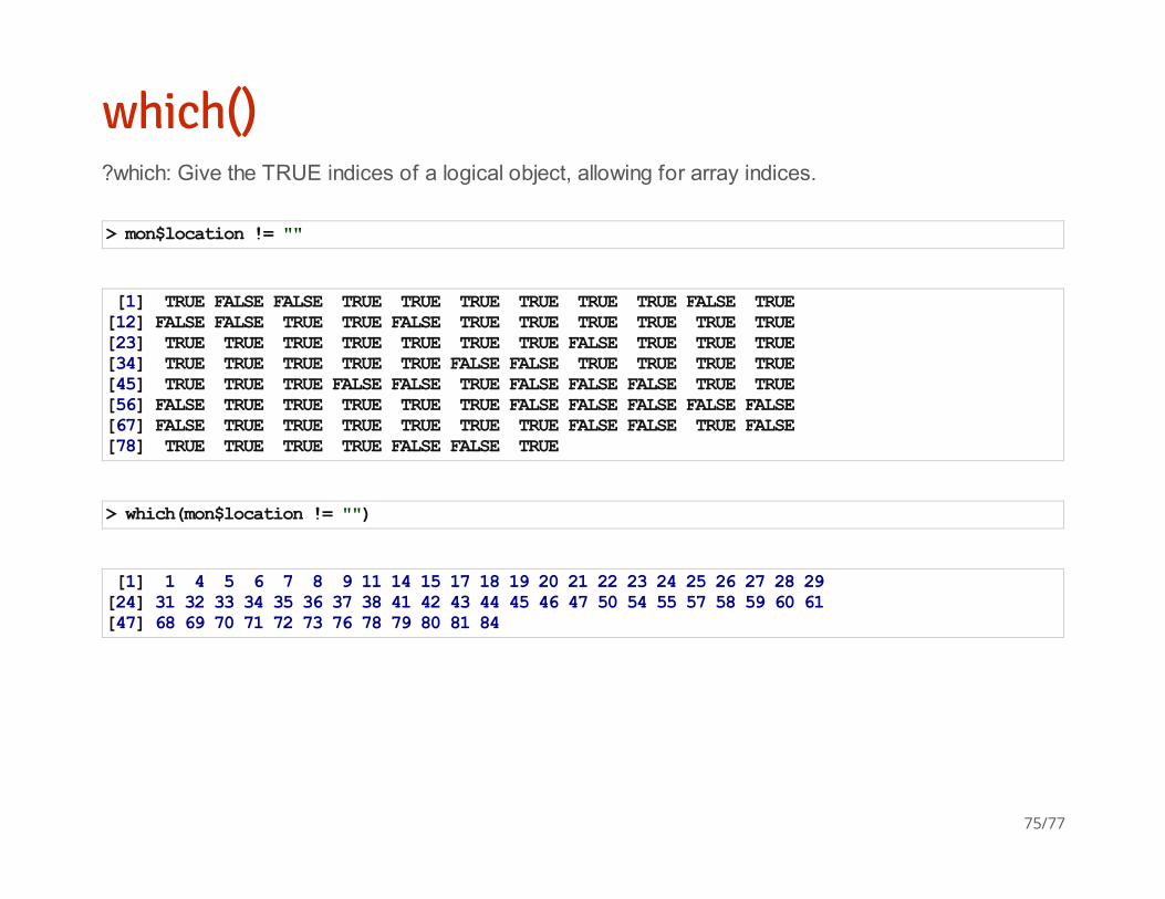
which()?which: Give the TRUE indices of a logical object, allowing for array indices.

> mon$location != ""

[1] TRUE FALSE FALSE TRUE TRUE TRUE TRUE TRUE TRUE FALSE TRUE[12] FALSE FALSE TRUE TRUE FALSE TRUE TRUE TRUE TRUE TRUE TRUE[23] TRUE TRUE TRUE TRUE TRUE TRUE TRUE FALSE TRUE TRUE TRUE[34] TRUE TRUE TRUE TRUE TRUE FALSE FALSE TRUE TRUE TRUE TRUE[45] TRUE TRUE TRUE FALSE FALSE TRUE FALSE FALSE FALSE TRUE TRUE[56] FALSE TRUE TRUE TRUE TRUE TRUE FALSE FALSE FALSE FALSE FALSE[67] FALSE TRUE TRUE TRUE TRUE TRUE TRUE FALSE FALSE TRUE FALSE[78] TRUE TRUE TRUE TRUE FALSE FALSE TRUE

> which(mon$location != "")

[1] 1 4 5 6 7 8 9 11 14 15 17 18 19 20 21 22 23 24 25 26 27 28 29[24] 31 32 33 34 35 36 37 38 41 42 43 44 45 46 47 50 54 55 57 58 59 60 61[47] 68 69 70 71 72 73 76 78 79 80 81 84

75/77

Missing Data

This will help you with the homework: http://www.statmethods.net/input/missingdata.html

In R, missing data is represented by the symbol NA (note that it is NOT a character, and therefore

not in quotes)

is.na() is a logical test for which variables are missing

Many summarization functions do not the calculation you expect (e.g. they return NA) if there is

ANY missing data, and these ofen have an argument 'na.rm=FALSE'. Changing this to

'na.rm=TRUE' will ignore the missing values in the calculation (i.e. mean(), sd(), max(), sum())

·

·

·

76/77

R classesYou can test whether an R object is a specific class. For example:

is.character(object)

is.integer(object)

is.numeric(object)

is.factor(object)

is.matrix(object)

is.data.frame(object)

·

·

·

·

·

·

77/77