Lecture 1

1

Introduction to Vehicle Crashworthiness

Lecture -1Lecture 1

CE 264Non-linear Finite Element Modeling and Simulation

Contact Information

Pradeep MohanOffice Phone: (703)726-8538Office Phone: (703)726-8538Office: Research 2, 302 EEmail: [email protected] Hours: 2:00 to 4:00 PM on

Tuesdays and by appointmentWeb: http://crash.ncac.gwu.edu/pradeep/

CE 264, Lecture 1 Slide #2

What is Non-Linear FEM and why study it? FEM is a numerical analysis technique for obtaining

approximate solutions to a wide variety of engineering problems for which an analytical solution does not

Objective

problems for which an analytical solution does not exist

Non-linearities Material

• Stress-strain behavior Geometry


• Change in geometry have a significant effect on the load deformation behavior

Safety Standards


2

Federal Motor Vehicle Safety Standards (Part 571)

“Active Safety / Crash Avoidance” - 100 Series Pre-Crash Phase

• Crash Avoidance & security Braking (ABS), electronic stability control (ESC), lighting and signalling

“Passive Safety / Crashworthiness” - 200 Series Crash Phase

• Minimize risk of injury to occupants, combines the reciprocal aims of absorbing impact and ensuring a survival space

208 – Occupant Crash Protection 214 – Side Impact Protection 216 – Roof Crush Resistance


“Fire-related” - 300 Series Post-Crash Phase

• Interior Trim Flammability and fuel system integrity 301 – Fuel System Integrity

Frontal Impact – Regulatory Requirements

Federal Motor Vehicle Safety Standard (FMVSS) 208 – old

30 mph ( 48 kph) into a fixed barrierbarrier

50th percentile Hybrid III dummy in front driver and passenger seats

Uses dummy injury measures for regulation

• Chest G’s <= 60• HIC <= 1000• Femur Loads <= 10 KN

Protection must be automatic


Protection must be automatic

Purpose of this test is to evaluate the performance of the occupant restraint systems (seat belts, airbags, etc.)

FMVSS 208 – New Regulation

The first stage phase-in ,9/1/03-8/31/06, requires vehicles to be certified as passing: Unbelted test requirements for both the 5th percentile

d lt f l d 50th til d lt l d i iadult female and 50th percentile adult male dummies in a 40 km/h (25 mph) rigid barrier crash

Belted test requirements for the same two dummies in a rigid barrier crash with a maximum test speed of 48km/h (30 mph)

Include technologies that will minimize risk for young


children and small adults • De-powered Airbags• Occupant sensing system


The second stage phase-in, 9/1/ 2007-8/31/2010, requires vehicles to be certified as passing: Maximum test speed for the belted rigid barrier test

will increase from 48 km/h (30 mph) to 56km/h (35will increase from 48 km/h (30 mph) to 56km/h (35 mph) in tests with the 50th percentile adult male dummy only


3


Test requirements to improve occupant protectionfor different size occupants, belted and unbelted

50th precentileadult male dummies

5th percentileadult female dummy

Rigid Barrier Test Rigid Barrier Test 40% offset frontaldeformable barrier test

UnbeltedDriver andP

BeltedDriver andP

UnbeltedDriver andP

BeltedDriver andP

BeltedDriver andP


Passenger20-25 mph

Passenger0-35 mph

Passenger20-25 mph

Passenger0-30 mph

Passenger0-25 mph

Perpendicularand up to 30

degreesOblique

Perpendicular Perpendicular Perpendicular Left SideImpact


Test requirements to minimize the risk to infants,children, and other occupants from injuries and

deaths caused by airbags

Rear facing childsafety with 1 year

old dummy

3-year-oldand 6-year-oldchild dummies

Suppression(presence)

Suppression(presence)

Suppression(out of position)

5th percentile adultfemale dummy(driver position)


Low riskdeployment

Low riskdeployment

Suppression(out of position)

Low riskdeployment

FMVSS 208 – Advanced occupant protection

FMVSS 208 drove design changes to adjust the deployment of the front airbags to enhance protection for front-seat occupants using crash severity sensors crash severity sensors seat belt usage sensors dual-stage driver and front-passenger airbags driver's seat position sensor front outboard safety belt pre-tensioners etc.,


Frontal Impact – Consumer Tests New Car Assessment Program, NCAP

• 35 mph (56 kph) into a fixed rigid barrier

• 50th percentile Hybrid III dummy in front driver and passenger seats

= 10% or less chance of serious injury

= 11% to 20% chance of serious injury

= 21% to 35% chance of serious injury p g

• Star rating used to assess probability of serious injury

• Head and chest injury data are combined into a single rating and reflected by the number of stars

j y= 36% to 45% chance

of serious injury = 46% or greater

chance of serious injury


4

Frontal Impact - Consumer Tests

Insurance Institute for Highway Safety (IIHS)

40% offset 40 mph (64 kph) into 40% offset 40 mph (64 kph) into a deformable barrier

50th percentile male Hybrid III dummy in front driver seat

Good, Acceptable, Marginal and Poor ratings to assess vehicle’s overall crashworthiness

Rating based on:


• Dummy Injury measures• Structural performance• Restraints/dummy

kinematics

Evaluates the structural performance of the vehicle

Federal Motor Vehicle Safety Standard (FMVSS) 214

33.5 mph (54kph) crabbed impact

Side Impact – Regulatory Requirements

impact Impactor mass - 3015 lb US SID dummy in front and

rear seats Uses dummy injury measures

for regulation TTI(d) <= 85g for LTV’s and 4

door passenger cars TTI(d) <= 90g for 2 door

passenger cars


p g Pelvic Acceleration <= 130g TTI(d) = 0.5 X (Gr + Gs)

• Gr = Max. Rib Acc. • Gs = Lower spine Acc

Side Impact - Consumer Tests

Lateral/Side Impact New Car Assessment Program (LINCAP or SINCAP)

NHTSA issued an NPRM for side impact on May 19, 2004

59% of fatalities in side impact 38.5 mph (62kph) crabbed

impact 3015 lb (1370 Kg) impactor

mass SID dummy in front and rear

seats (SID/HIII for vehicles with side airbags)

Star rating based on TTI Pelvic Acceleration <= 130g

phad a brain injury

Promote head protection for all vehicle classes

20mph closing speed at 750

anticlockwise angle of approach into a rigid pole*

SID-IIs will be tested with the moving barrier and the oblique pole*

ES 2re to replace US DOT SID


Thoracic Trauma Index5 Stars <=524 Stars 57-723 Stars 72-912 Stars 91-981 Star 98 >=

ES-2re to replace US DOT SID

* Most likely


Insurance Institute for Highway Safety

New test implemented in Fall New test implemented in Fall 2003

Impactor mass - 1,500 Kg Impactor shape derived from

Ford F150 front profile 50 km/h perpendicular impact SIDII’s driver and rear passenger

dummies Seated using UMTRI seating

position


position

5


Purpose is to represent crash condition that poses


Purpose is to represent crash condition that poses greatest risk to occupants (Pick-up/SUV as striking vehicle)

Promote head protection

Rear Impact – Regulatory Requirements

Federal Motor Vehicle Safety Standard (FMVSS) 301

The purpose of this standard is to reduce deaths and injuries occurring from fires that result from fuel spillage during and after motor vehicle crashes

30 mph ( 48 kph) with a rigid rear moving barrier 50th percentile Hybrid III dummy in front driver and passenger

seats Vehicle is rotated on its longitudinal axis to each successive


Vehicle is rotated on its longitudinal axis to each successive increment of 900 and fuel spill is measured

Brief Introduction to Finite Element Methods


Source: Finite Element Primer for EngineersSource: Finite Element Primer for EngineersMike Barton & S. D. Rajan (Arizona state univ.)

Finite Element Method

Many problems in engineering and applied science are governed by differential or integral equations.

Th l i h i ld id The solutions to these equations would provide an exact, closed-form solution to the particular problem being studied.

However, complexities in the geometry, properties and in the boundary conditions that are seen in most


and in the boundary conditions that are seen in most real-world problems usually means that an exact solution cannot be obtained or obtained in a reasonable amount of time.

6


Current product design cycle times imply that engineers must obtain design solutions in a ‘short’ amount of time.

They are content to obtain approximate solutions that can be readily obtained in a reasonable time frame, and with reasonable effort. The FEM is one such approximate solution technique.


The FEM is a numerical procedure for obtaining approximate solutions to many of the problems encountered in engineering analysis.

Finite Element Method In the FEM, a complex region defining a continuum is

discretized into simple geometric shapes called elements.

The properties and the governing relationships are assumed o er these elements and e pressed mathematicall in termsover these elements and expressed mathematically in terms of unknown values at specific points in the elements called nodes.

An assembly process is used to link the individual elements to the given system. When the effects of loads and boundary conditions are considered, a set of linear or nonlinear algebraic equations is usually obtained


algebraic equations is usually obtained.

Solution of these equations gives the approximate behavior of the continuum or system.


The continuum has an infinite number of degrees-of-freedom (DOF), while the discretized model has a finite number of DOF. This is the origin of the name, finite element method.

The number of equations is usually rather large for most real-world applications of the FEM, and requires the computational power of a super computer. The FEM has little practical value if super computers were not available.

Advances in and ready availability of computers and software h b ht th FEM ithi h f i ki i


has brought the FEM within reach of engineers working in small industries, and even students.


Two features of the finite element method are worth noting.

The piecewise approximation of the physical field The piecewise approximation of the physical field (continuum) on finite elements provides good precision even with simple approximating functions. Simply increasing the number of elements can achieve increasing precision.

The locality of the approximation leads to sparse i f di i d bl Thi


equation systems for a discretized problem. This helps to ease the solution of problems having very large numbers of nodal unknowns. It is not uncommon today to solve systems containing a million primary unknowns.

7

Origin of FEM

It is difficult to document the exact origin of the FEM, because the basic concepts have evolved over a period of 150 or more years.

The term finite element was first coined by Clough in 1960. In the early 1960s, engineers used the method for approximate solution of problems in stress analysis, fluid flow, heat transfer, and other areas.

The first book on the FEM by Zienkiewicz and Chung was bli h d i 1967


published in 1967.

In the late 1960s and early 1970s, the FEM was applied to a wide variety of engineering problems.

Origin of FEM

The 1970s marked advances in mathematical treatments, including the development of new elements, and convergence studies.

Most commercial FEM software packages originated in the 1970s (ABAQUS, ADINA, ANSYS, MARK, PAFEC) and 1980s (FENRIS, LARSTRAN ‘80, SESAM ‘80.)

The FEM is one of the most important developments in computational methods to occur in the 20th century. In just a f d d th th d h l d f ith


few decades, the method has evolved from one with applications in structural engineering to a widely utilized and richly varied computational approach for many scientific and technological areas.

Advantages of FEM The FEM offers many important advantages to the design

engineer:

Easily applied to complex, irregular-shaped objects composed of se eral different materials and ha ing comple bo ndarof several different materials and having complex boundary conditions.

Applicable to steady-state, time dependent and eigenvalue problems.

Applicable to linear and nonlinear problems.


One method can solve a wide variety of problems, including problems in solid mechanics, fluid mechanics, chemical reactions, electromagnetics, biomechanics, heat transfer and acoustics, to name a few.

Sources of Error in FEM

The three main sources of error in a typical FEM solution are discretization errors, formulation errors and numerical errors.

Discretization error results from transforming the physical system (continuum) into a finite element model, and can be related to modeling the boundary shape, the boundary conditions, etc.

Formulation error results from the use of elements that don't precisely describe the behavior of the h i l bl


physical problem. Numerical error occurs as a result of numerical

calculation procedures, and includes truncation errors and round off errors

8

General FEA Process

Model Development - Pre-processing Discretize Geometry: Nodes/Elements Geometry properties: Thickness/Cross-section Material properties Loading conditions Constraints Boundary conditions


Solver - Solution processing Numerical solution of equations of motion

General FEA Process

Post-processing: Results Analysis Deformed geometry Displacements, velocities, accelerations Stress and strain Reaction forces Energies

FE Model Improvement


Update Model based on the analysis results Iterative process until objectives achieved

General FEA Process

Model Development - Pre-processing LS-INGRID, FEM-B I-DEAS, True-Grid, EasiCrash, , PATRAN, HyperMesh

Solver - Solution processing LS-DYNA, PamCrash, RADIOSS NASTRAN, ANSYS, Algor

Results Analysis - Post-processing


y p g LS-TAURUS, LS-POST HyperMesh

Background and History of LS-DYNA

1976 DYNA3D developed at Lawrence Livermore National

Laboratory by John HallquistL l it i t f h lid t t ilit Low velocity impact of heavy, solid structures, military applications

1979 DYNA3D ported on Cray-1 Improved sliding interface Order of magnitude faster


Order of magnitude faster 1981

New material models - Explosive-structure, Soil-structure

Impacts of penetration projectiles

9


1986 Beams, Shells, Rigid Bodies Single Surface Contact Single Surface Contact Support for Multiple Computer Platforms

1988 Automotive Applications Support LS-DYNA

1989


1989 Full Commercial Version LSTC


1993 Keyword Format Automatic Single Surface Contact 1st International LS-DYNA User Conference

1995 Training Lab Established at West Coast - LSTC

1997


Training Class Started at East Coast - NCAC/GWU Today

Release of Version LS971, Many New Features

General Capabilities

Transient dynamics Quasi-static simulations Flexible and rigid bodiesg Nonlinear material behavior More than 80 constitutive relationships More than 40 element formulation Finite strain and finite rotation General contact algorithm


Thermal Analysis Explicit and implicit analyses

Applications

Automotive, train, ship, and aerospace crashworthinessSheet and b lk forming process sim lation Sheet and bulk forming process simulation

Engine blade containment and bird strike analysis Seismic safety simulation Weapons design and explosive detonation simulation Biomechanics simulation


Industrial accidents simulation Drop and impact analysis of consumer product Roadside Hardware Analysis Virtual proving ground simulation

10

LS-DYNA Input File Format

Structured Input Format Original Format Organized by Entities

Fi d F t Fixed Format Keyword Input Format

Started 1993 More Flexible Easy to Modify Input Deck


Keyword Format Input File

*KEYWORD*TITLESAMPLE INPUT FILE *CONTROL_TERMINATION0.1000000 0 0.0000000 0 0.0000000

*NODE1 0.000000000E+00 0.000000000E+00 0.000000000E+002 7.000000000E+00 0.000000000E+00 0.000000000E+003 0.000000000E+00 7.000000000E+00 0.000000000E+00 4 7.000000000E+00 7.000000000E+00 0.000000000E+00

*DATABASE_BINARY_D3PLOT1.00000-3 0*DATABASE_BINARY_D3THDT1.00000-3*MAT_ELASTIC

1 7.89000-9 2.00000+5 0.3000000*SECTION_SOLID

1 0*SECTION_SHELL

1 21 0000000 1 0000000 1 0000000 1 0000000 0 0000000

5 0.000000000E+00 0.000000000E+00 7.000000000E+006 7.000000000E+00 0.000000000E+00 7.000000000E+007 0.000000000E+00 7.000000000E+00 7.000000000E+008 7.000000000E+00 7.000000000E+00 7.000000000E+00

*ELEMENT_SOLID1 1 1 2 4 3 5 6 8 7

*PARTPART NAME 1

2 2 2 0 0 0 0 0*ELEMENT_SHELL

1 2 1 2 4 3


1.0000000 1.0000000 1.0000000 1.0000000 0.0000000*PARTPART NAME 1

1 1 1 0 0 0 0 0

1 2 1 2 4 3*END

Keyword Format Input File Sections

Control, Material, Equation of State, Element, Parts, etc.

The “*” followed by keyword indicate beginning of a The followed by keyword indicate beginning of a section block.

The “$” used for Comment Cards Data blocks begin with keyword followed by data

pertaining to the keyword Multiple Blocks with the same keyword are


p ypermissible

Material and Contact types are defined by name Keywords are alphabetically organized in manual

Keyword Format Input File

*NODE NID x y z

*ELEMENT EID PID N1 N2 N3

*PART PID SID MID EOSID HGID

*SECTION_SHELL SID ELFORM SHRF NIP PROPT QR ICOMP

*MAT_ELASTIC MID RO E PR DA DB


*EOS EOSID

*HOURGLASS HGID

11

LS-DYNA Execution

Command Line

Examplels-dyna i=inputfile


ls940 r=d3dump01 memory=12000000ls971s i= inputfile

LS-DYNA Execution


LS-DYNA Output Files

d3hsp message d3plot,d3plot01,… d3thdt,d3thdt01, … d3dump01, … runrsf Ascii files (glstat, nodout, deforc, ..etc)


(g )

CAE Influence on Vehicle Development Process (VDP)


12

History of Numerical Simulations

Explicit FE codes were developed in the 60’s and 70’s at the Defense Labs in the US

First full vehicle car crash models were built and l d i th id 80’ h j tanalyzed in the mid 80’s as a research project

Introduction of supercomputers (cray) made it possible to run a full vehicle crash model

Development of the codes continue to make numerical solutions stable and accurateNumerical simulation has become a fully integrated


Numerical simulation has become a fully integrated tool in the vehicle development process in the last decade

History of Numerical Simulations

Difficult to conceive a vehicle design with today’s constraints of regulations and safety without any simulation at allAccurate and robust analytical tools using state of Accurate and robust analytical tools using state-of-the-art in computational mechanics and computer hardware are indispensable for crash simulations

The contribution of simulation lies in that it complements a testing facility by preventing unnecessary work from being done


y g The ideal picture is indeed one of a design, heavily

supported by analysis, resulting in building of only those prototypes that are almost certain to pass all final verification testing

Evolution of CAE in Crashworthiness

RegulatoryRequirements

FE ModelSize (elem)

Prototypes reqd. for crash testing

1985 1 10000 150

Year

1990

1995

2000

5

20000

80000

0 5M Mad

e po

ssib

le b

y up

erco

mpu

ters

120

100

50 ifica

nt c

ost s

avin

gs

Red

uce

Inju

ries &

Fata

litie

s


All numbers shown here are estimates only,and should be treated as such

2000

Today >20

0.5M

>1M

M su 50

<20

Sign

i

Engineering Analysis

Engineering Analysis Methods

Numerical methodsClassical methods

Exact Approximate EnergyBoundaryElement

Finite Difference

Finite Elements


CAE: Uses Engineering analysis tools primarily FE, BE and FD methods

Linear / Non-Linear: based on material, loadingStatic / Dynamic: Temporal variation in loading, boundary conditions Quasi Static /Transient are sub-cases of above

13

FE Crashworthiness

FE crashworthiness analysis of vehicles in particular, is among the most challenging nonlinear problems in structural mechanicsVehicle structures are typically manufactured from Vehicle structures are typically manufactured from many stamped thin shell parts and subsequently assembled by various welding and fastening techniques

The body-in-white may contain steel of various strength grades, aluminum and/or composite


g gmaterials

• Validation of Structure: Component, Subsystem and System

• Ride Comfort: NVH, Cabin Acoustics, Passenger Efforts (eg: Door opening)

• Handling: Vehicle Dynamics Analysis, Kinematics

Automotive CAE requirements

Handling: Vehicle Dynamics Analysis, Kinematics

• Safety: Crash (Front, Rear, Side, Roof)

• Durability: Life of components during real-life vehicle loading of variable severity, Fatigue life-cycle analysis

• Fuel Economy, Aerodynamics


• Cross-functional as well as individual optimizations for cost, weight and investment (CWI)

Pre–processing (FE modeling):

Hypermesh: Standard for Automotive CAE modeling ( good for solid modeling, auto/manual meshing edits and all quality checks)

ANSA: Superior to HM for Shell meshing and assembly but inferior for solid models

Automotive CAE Tools

Others: Easi-Crash, LS-Pre, Oasys, I-DEAS, PATRAN

Solvers:

MSC NASTRAN: Best in class for Linear, dynamic and optimization type analyses (best for NVH, Durability)

LS-DYNA: Non-Linear, large deformation, Crash type analysisADAMS: Vehicle dynamicsMADYMO: Occupant simulation


MADYMO: Occupant simulationOther: ANSYS (multi-physics problems)

Post-processing:

LS-POST, Hyperview, Easi-Crash etc.,

StrategicDirection

ProgramStart

ConfirmProgramVision

Concept Selection& Major Hardpoints

Approval:Theme

SelectionTheme

Confirmation Prototype S0 Start S1 StartVolumeProd.

Week WeekWeek

48 month VDP

Pre-Program

ReferenceBaseline

Digital Mule Theme

DORs

DOR+

DigitalPrototype

Post S0Refinement

1st physicalValidation

208WBVP

Week80

Week150


Phase Main window for Digital/Virtual Vehicle

development Validation Phase

prototype

Program name(sample): 02LH

14

StrategicDirection

ProgramDefinition

PD

Program Implement

P1

ThemeDecision

TD

Program Confirm

PC

PrototypeConfirmDesign

CP S0 LR J1Program Redesign

PR

48 month VDP

• Design Alternatives• Major Architectural

ArchitectureSelected

Clay modelcomplete

Month48

324Month43

3337StructuralPrototype

SP

21 17 727

Engineering& Manufacturing

sign off


jChanges

• High Design Freedom• High CAE contributions• Limited Vehicle specificdata

• Design specs available• Minor modifications to design• Lower design freedom• More of optimization followingredesign to targets

• Full Design specs available• Tuning with prototype testing• Proving ground data• CAE in reactive and correlationmode

Influence on Vehicle Safety

2001 Model Year 2004 Model Year


Crashworthiness Model Requirements

The models should satisfy at a minimum the following overall requirements: Accuracy – the model should be able to yield

reasonably accurate predictions of the essential y pfeatures being sought

Speed – the model should be executable with a reasonable turnaround time, not to exceed 12 hours regardless of its size, to allow for iterations and parameter studies

Robustness – small variations in model parameters should not yield large variations in model responses


should not yield large variations in model responses Development time – the model should be built in a

reasonably short period of time, not to exceed two weeks

Structure Design for Crashworthiness


15

Automotive Body


Automotive Body - Structure

Two types of body structures (Body-In-White) Unibody (passenger car) Ladder frame (trucks/SUV) Ladder frame (trucks/SUV)


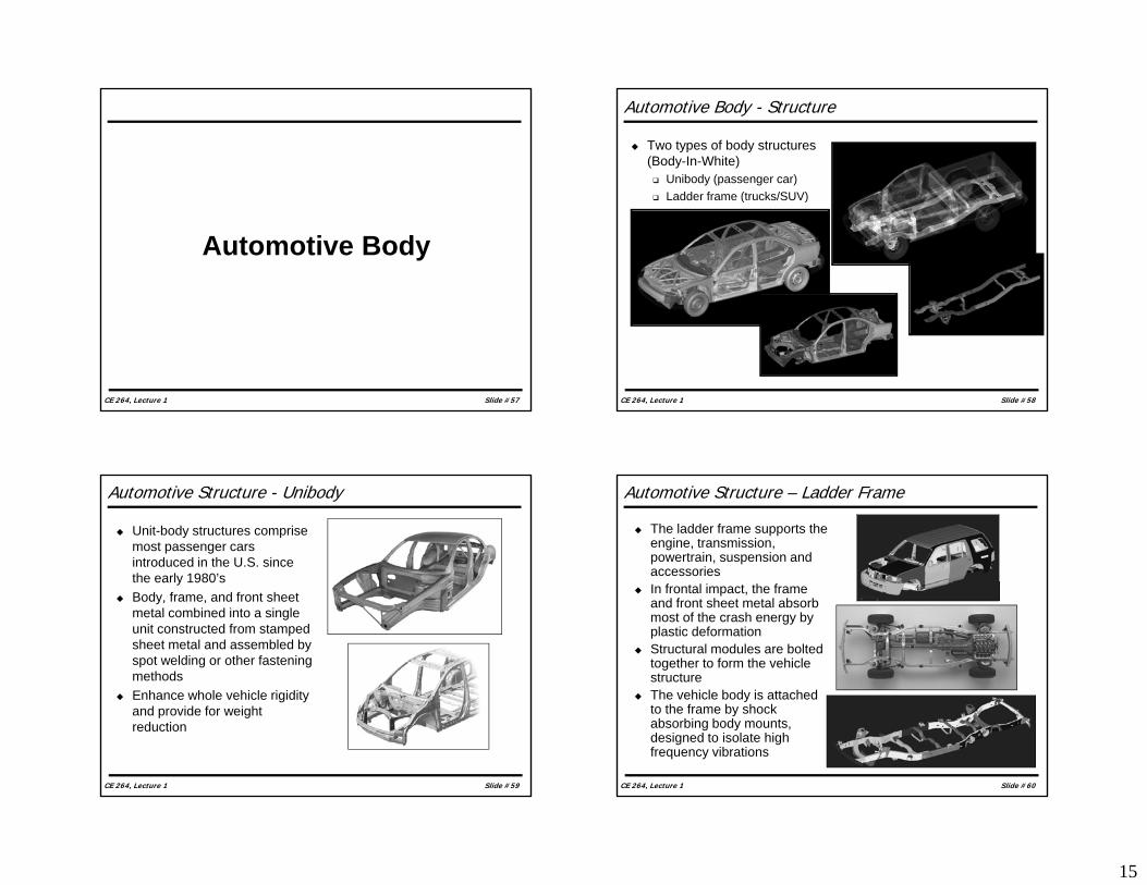
Automotive Structure - Unibody

Unit-body structures comprise most passenger cars introduced in the U.S. since the early 1980’sthe early 1980 s

Body, frame, and front sheet metal combined into a single unit constructed from stamped sheet metal and assembled by spot welding or other fastening methods


Enhance whole vehicle rigidity and provide for weight reduction

Automotive Structure – Ladder Frame

The ladder frame supports the engine, transmission, powertrain, suspension and accessories

In frontal impact, the frame and front sheet metal absorb most of the crash energy by plastic deformation

Structural modules are bolted together to form the vehicle structure


The vehicle body is attached to the frame by shock absorbing body mounts, designed to isolate high frequency vibrations

16

Body-In-White (BWI)

Firewall – separates engine from compartment

Center Tunnel –d t th h t

Occupant Compartment

accommodates the exhaust pipes and drive-shaft

Sills – Profiled longitudinal beams designed in two shell construction

Side Frame – A,B,C and D pillars


Side Panel – External side panels

Floor Assembly – forms the back-bone for the entire body

Roof

Body-In-White (BWI)

Underframe/Cradle Used as an engine and/or

suspension mount

Front End

Provides torsional stiffness to the structure

Bolted through vibration dampers to the front rails

Cross member Strong welded steel or

magnesium structure (or


magnesium structure (or single cast piece)

Transfers energy to the opposite side in the event of a severe side or angular collision

Body-In-White (BWI)

Front rails most important part in the front

end structure Absorb a great deal of the

Front End

Absorb a great deal of the energy in a frontal crash (typically about 40 KN/rail for compact cars)

Complex and strong interaction with FBHP, firewall, etc..

Have crush initiators and deformation aids to crush in a controlled manner

Deformation Aid


controlled manner

Crush Initiators

Body-In-White (BWI)

Wheel Houses Extremely strong by virtue

of their shape

Front End

Incorporate strengtheners, beads, and offsets

Upper side member Positioned along the entire

length of the wheel houseAbsorbs additional energy


Absorbs additional energy during severe frontal collisions

Incorporate reinforcements

17

Body-In-White (BIW)

Simpler design compared to front

Based on a closed box design

Rear End

Rails are incorporated to dissipate energy

Panels around the wheelhouse provide additional support

Strong B-pillarsSide Protection


Door beams positioned to engage the barrier

Door trims have foam padding to minimize hard contact points on impact

Lecture 1

Documents

Transcript of Lecture 1