Lecture # 03Lecture # 03

Demand and Supply (cont.)Demand and Supply (cont.)

Lecturer: Martin ParedesLecturer: Martin Paredes

2

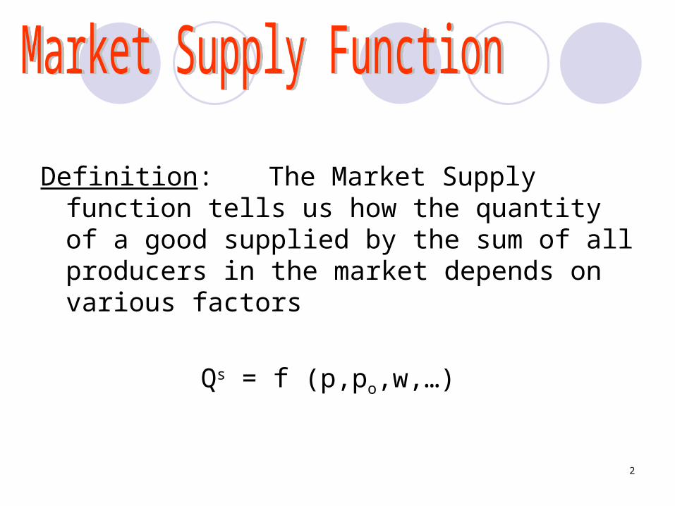
Definition: The Market Supply function tells us how the quantity of a good supplied by the sum of all producers in the market depends on various factors

Qs = f (p,po,w,…)

3

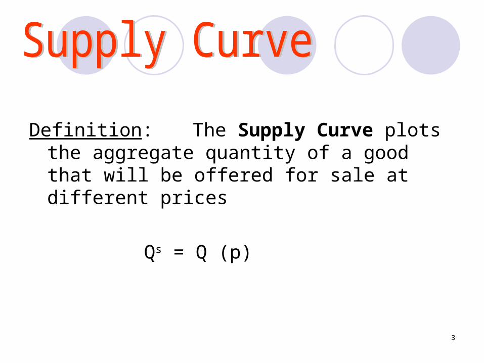
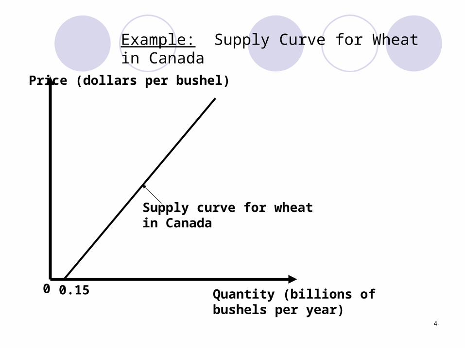
Definition: The Supply Curve plots the aggregate quantity of a good that will be offered for sale at different prices

Qs = Q (p)

4

Example: Supply Curve for Wheat in Canada

0 Quantity (billions ofbushels per year)

Price (dollars per bushel)

Supply curve for wheat in Canada

0.15

5

Definition: The Law of Demand Curve states that the quantity of a good offered increases when the price of this good increases. Empirical regularity

6

The supply curve shifts when factors other than own price change… If the change increases the willingness of

producers to offer the good at the same price, the supply curve shifts right

If the change decreases the willingness of producers to offer the good at the same price, the supply curve shifts left

7

A move along the supply curve for a good can only be triggered by a change in the price of that good.

A shift in the supply curve for a good can be triggered by a change in any other factor A change that affects the producers’

willingness to offer the good.

8

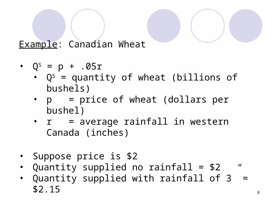
Example: Canadian Wheat

• QS = p + .05r• QS = quantity of wheat (billions of bushels)• p = price of wheat (dollars per bushel)• r = average rainfall in western Canada

(inches)

• Suppose price is $2 • Quantity supplied no rainfall = $2• Quantity supplied with rainfall of 3” = $2.15

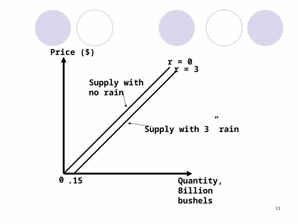
• As rainfall increases, supply curve shifts right• (e.g., r = 4 => Q = p + 0.2)

9

Price ($)

Quantity, Billion bushels

0

10

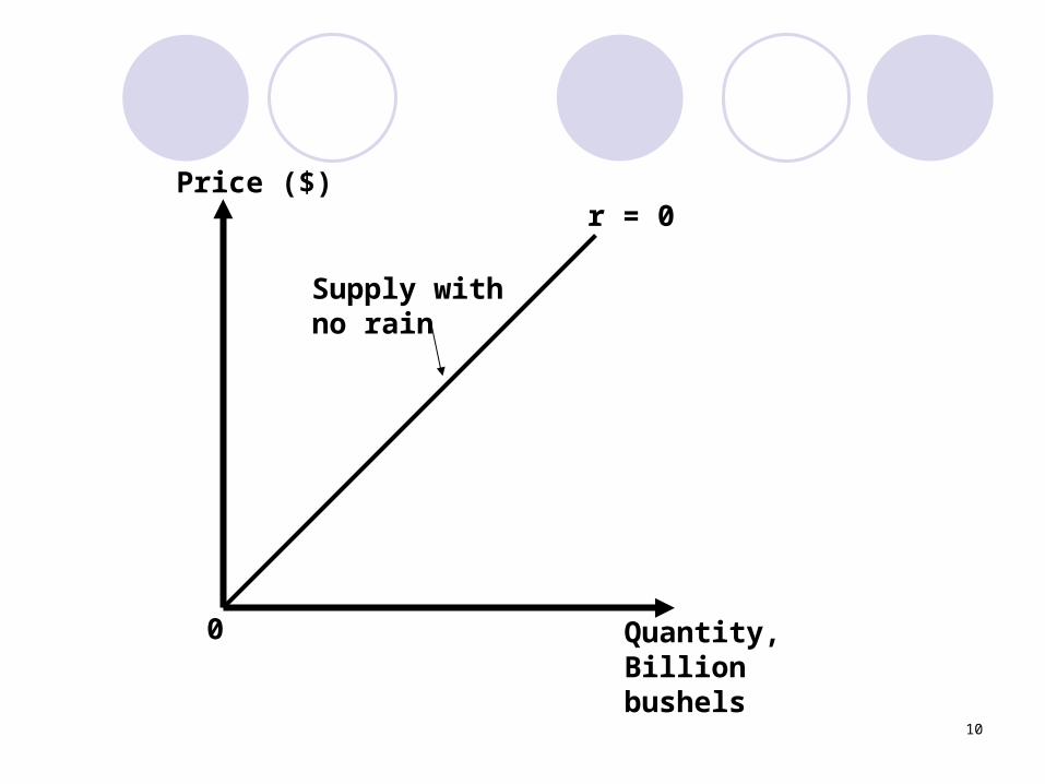
Price ($)

Quantity, Billion bushels

0

r = 0

Supply withno rain

11

Price ($)

Quantity, Billion bushels

0

r = 0r = 3

.15

Supply withno rain

Supply with 3” rain

12

Definition: A market equilibrium is a price such that, at this price, the quantities demanded and supplied are the same.

Demand and supply curves intersect at equilibrium.

13

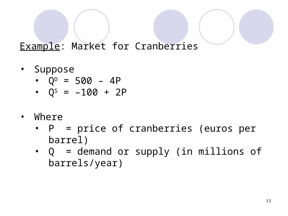
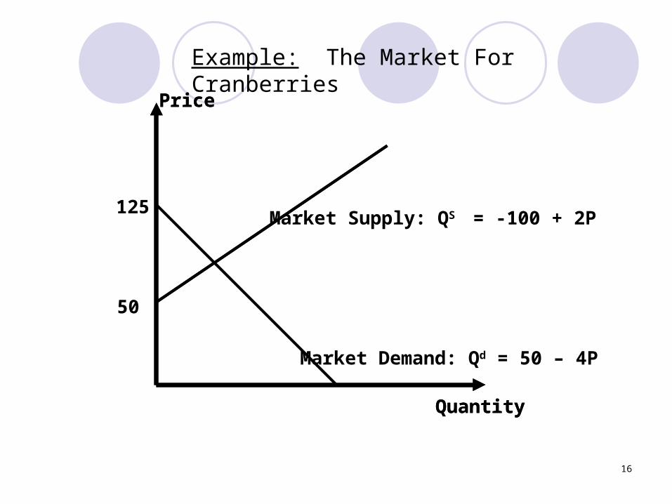
Example: Market for Cranberries

• Suppose• QD = 500 – 4P• QS = –100 + 2P

• Where• P = price of cranberries (euros per barrel)• Q = demand or supply (in millions of

barrels/year)

14

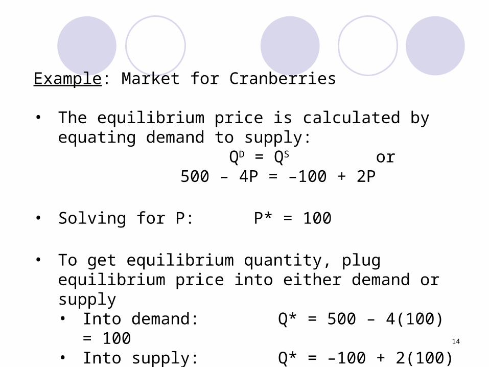
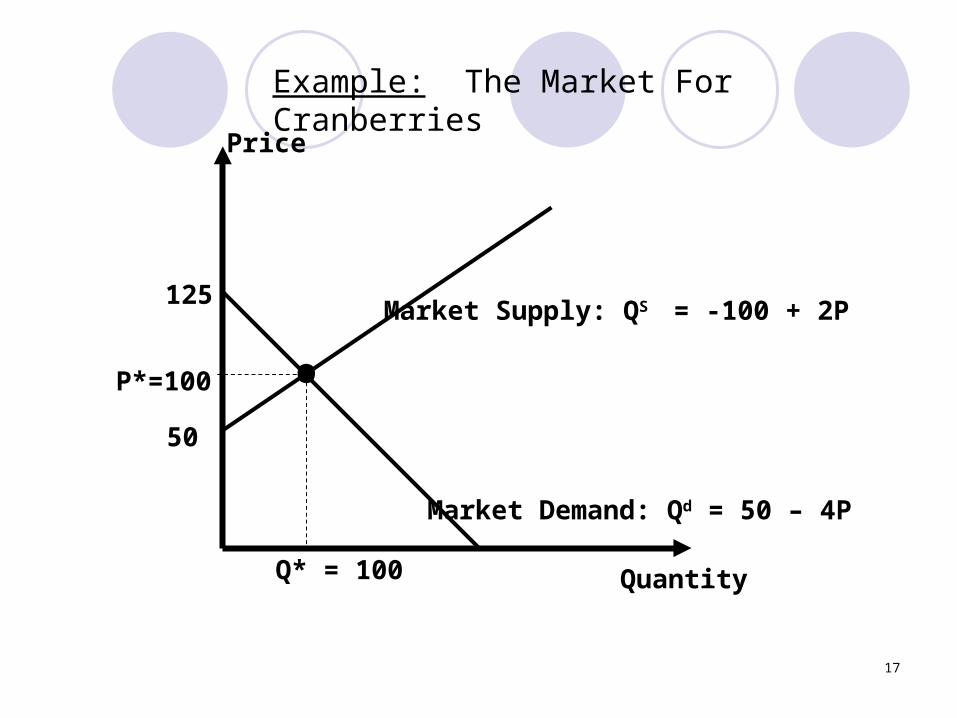
Example: Market for Cranberries

• The equilibrium price is calculated by equating demand to supply:

QD = QS or500 – 4P = –100 + 2P

• Solving for P: P* = 100

• To get equilibrium quantity, plug equilibrium price into either demand or supply• Into demand: Q* = 500 – 4(100) =

100• Into supply: Q* = –100 + 2(100) = 100

15

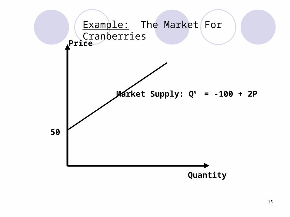
Example: The Market For Cranberries

Price

Quantity

Market Supply: QS = -100 + 2P

50

16

Price

Quantity

Price

Quantity

Market Demand: Qd = 50 – 4P

125

Example: The Market For Cranberries

Market Supply: QS = -100 + 2P

50

17

Price

QuantityQ* = 100

P*=100

125

•

Example: The Market For Cranberries

Market Supply: QS = -100 + 2P

50

Market Demand: Qd = 50 – 4P

18

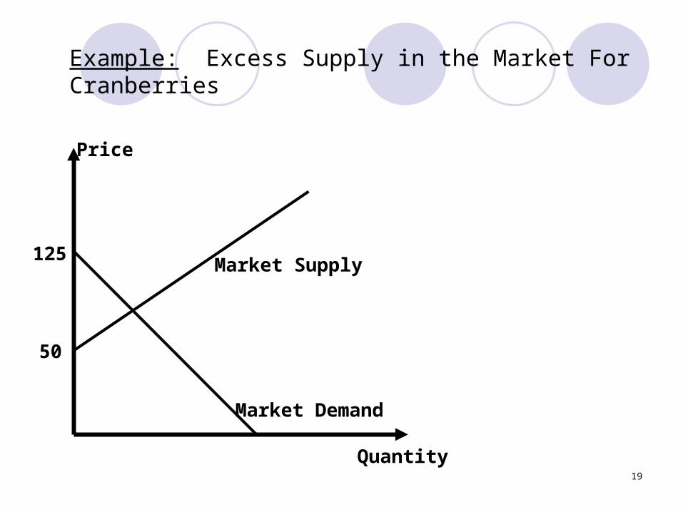
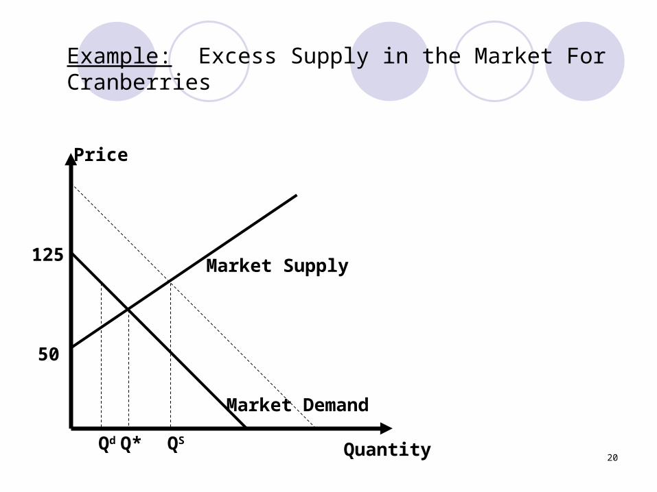
Definition: If at a given price, sellers cannot sell as much as they would like, there is excess supply.

Definition: If at a given price, buyers cannot purchase as much as they would like, there is excess demand.

19

Price

Quantity

Market Demand

Market Supply

50

125

Example: Excess Supply in the Market For Cranberries

20

Price

Quantity

Market Demand

Market Supply

Q*

50

125

QSQd

Example: Excess Supply in the Market For Cranberries

21

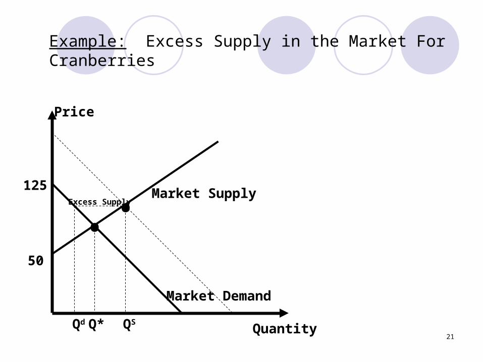
Price

Quantity

Market Demand

Market Supply

Q*

125Excess Supply

••

QSQd

50

Example: Excess Supply in the Market For Cranberries

22

If there is no excess supply or excess demand, there is no pressure for prices to change and we are in equilibrium.

When a change in an exogenous variable causes the demand curve or the supply curve to shift, the equilibrium shifts as well

23

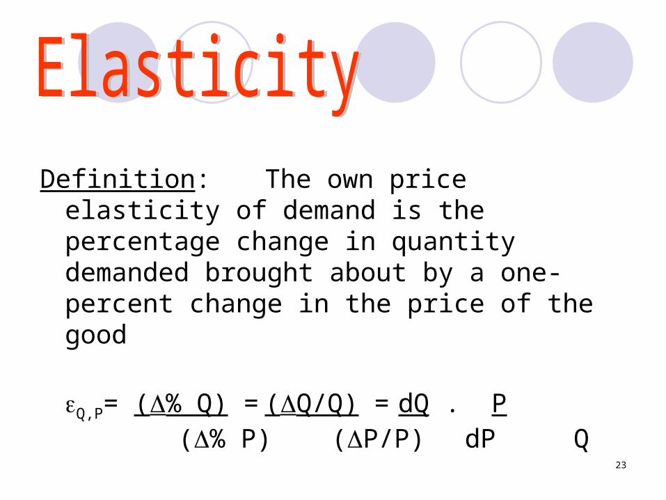
Definition: The own price elasticity of demand is the percentage change in quantity demanded brought about by a one-percent change in the price of the good

Q,P= (% Q) = (Q/Q) = dQ . P (% P) (P/P) dP Q

24

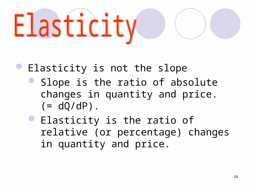
Elasticity is not the slope Slope is the ratio of absolute changes

in quantity and price. (= dQ/dP). Elasticity is the ratio of relative (or

percentage) changes in quantity and price.

25

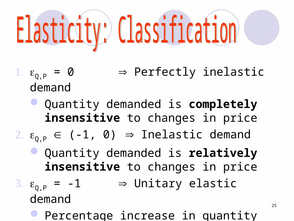
1. Q,P = 0 Perfectly inelastic demand Quantity demanded is completely

insensitive to changes in price2. Q,P (-1, 0) Inelastic demand

Quantity demanded is relatively insensitive to changes in price

3. Q,P = -1 Unitary elastic demand Percentage increase in quantity

demanded equals percentage decrease in price

26

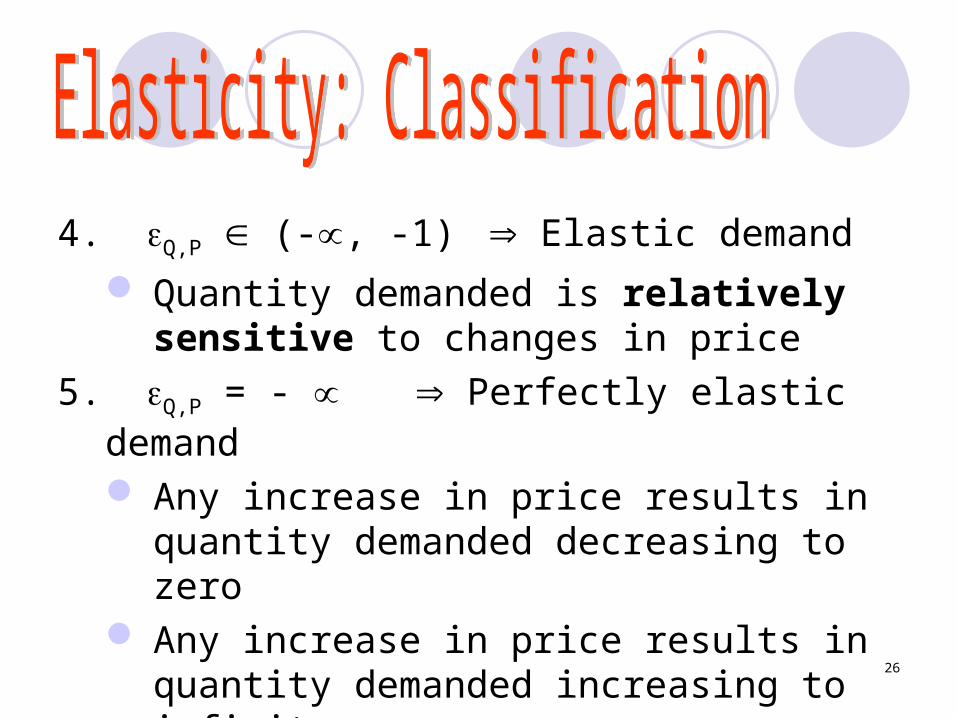
4. Q,P (-, -1) Elastic demand Quantity demanded is relatively

sensitive to changes in price5. Q,P = - Perfectly elastic demand

Any increase in price results in quantity demanded decreasing to zero

Any increase in price results in quantity demanded increasing to infinity.

27

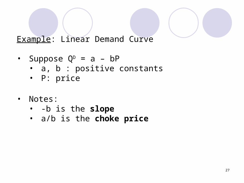
Example: Linear Demand Curve

• Suppose QD = a – bP• a, b : positive constants• P: price

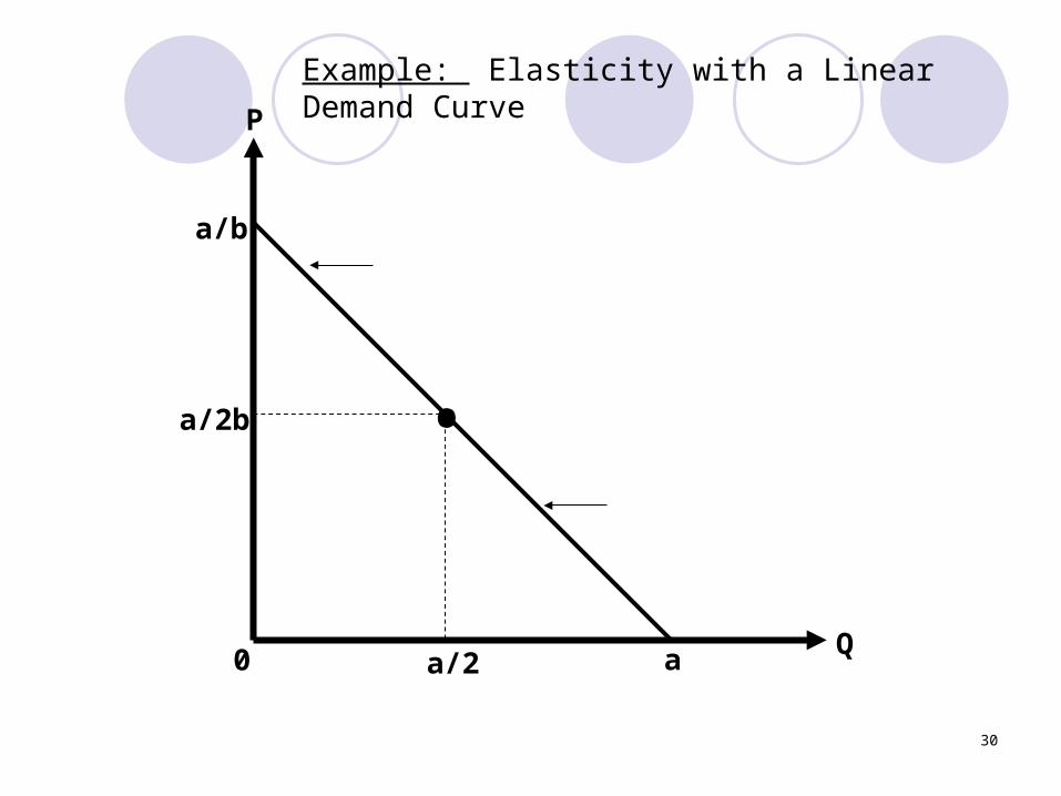
• Notes:• -b is the slope• a/b is the choke price

28

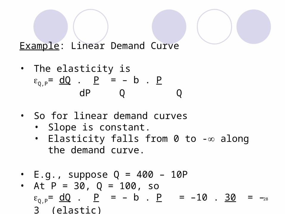
Example: Linear Demand Curve

• The elasticity isQ,P= dQ . P = – b . P

dP Q Q

• So for linear demand curves• Slope is constant. • Elasticity falls from 0 to - along the demand

curve.

• E.g., suppose Q = 400 – 10P• At P = 30, Q = 100, so

Q,P= dQ . P = – b . P = –10 . 30 = –3 (elastic) dP Q Q 100

29

0

P

Q

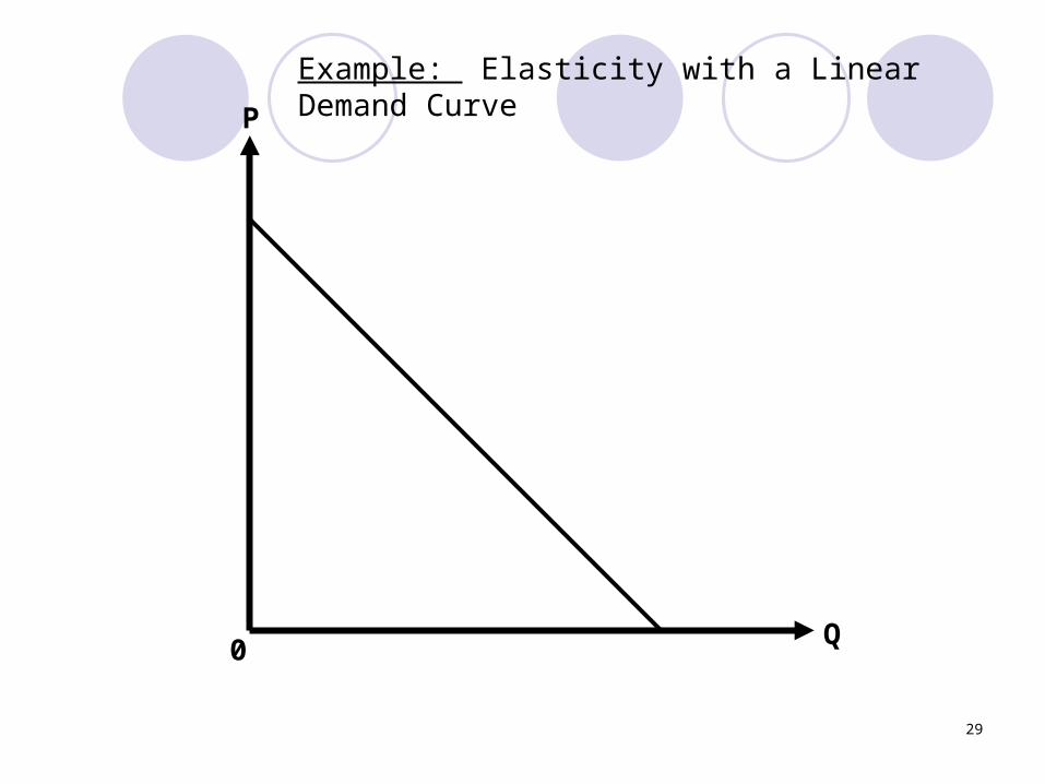
Example: Elasticity with a Linear Demand Curve

30

0

P

Qa/2 a

a/2b

a/b

•

Example: Elasticity with a Linear Demand Curve

31

0

P

Qa/2 a

a/2b

a/b

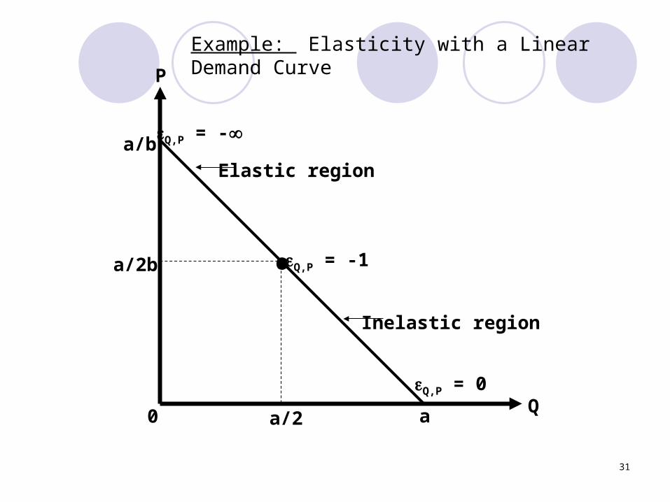
• Q,P = -1

Inelastic region

Elastic region

Q,P = -

Q,P = 0

Example: Elasticity with a Linear Demand Curve

32

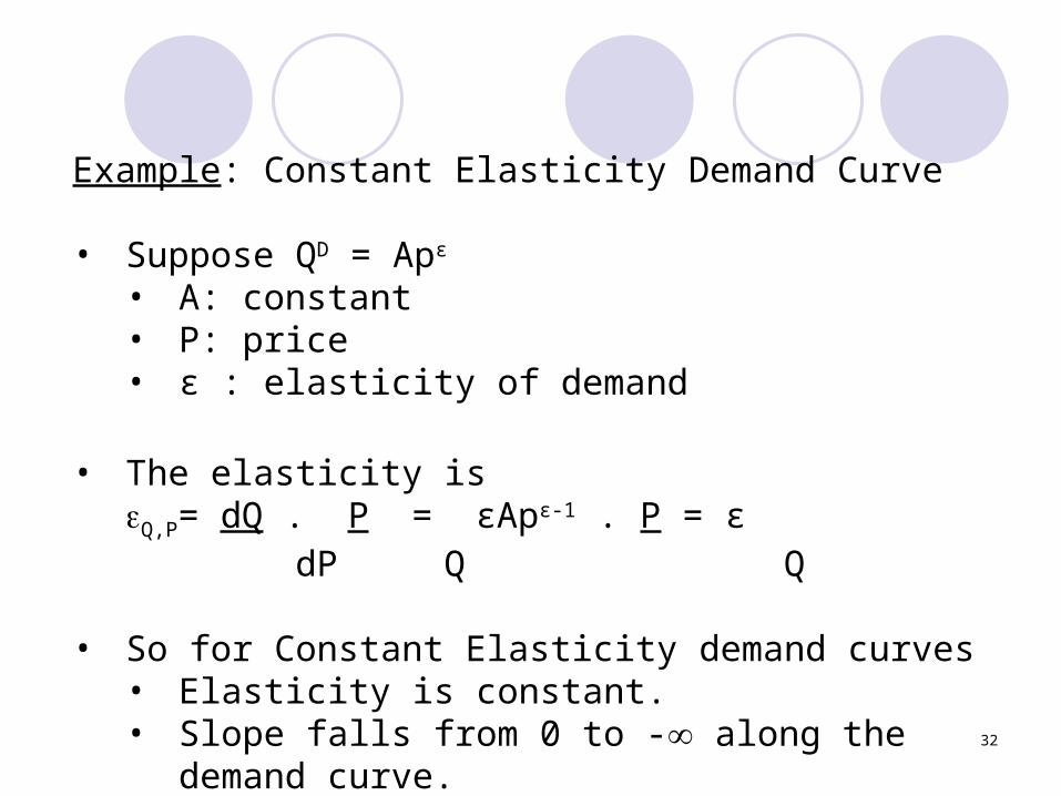
Example: Constant Elasticity Demand Curve

• Suppose QD = Apε

• A: constant• P: price• ε : elasticity of demand

• The elasticity isQ,P= dQ . P = εApε-1 . P = ε

dP Q Q

• So for Constant Elasticity demand curves• Elasticity is constant. • Slope falls from 0 to - along the demand

curve.

33

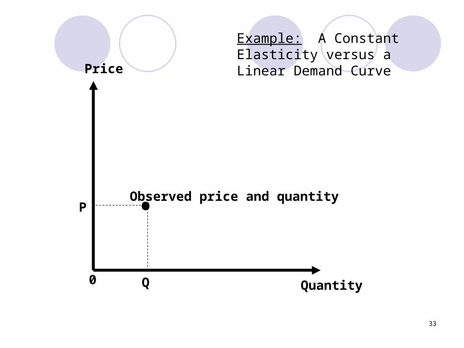
Quantity

Price

0 Q

P • Observed price and quantity

Example: A Constant Elasticity versus a Linear Demand Curve

34

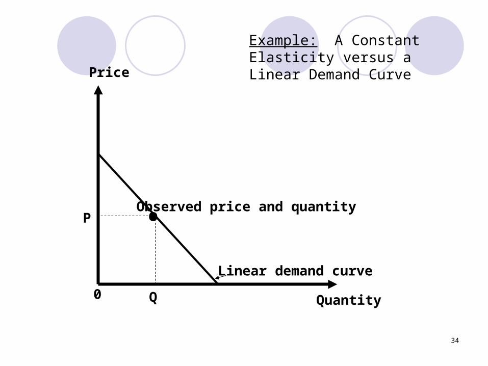
Quantity

Price

0 Q

P • Observed price and quantity

Linear demand curve

Example: A Constant Elasticity versus a Linear Demand Curve

35

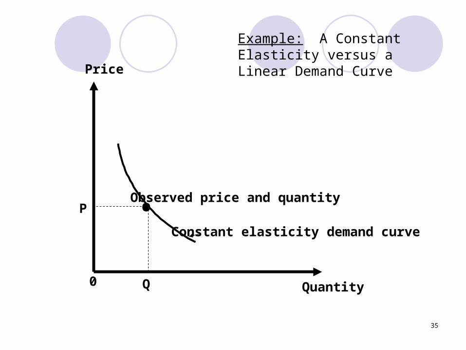
Quantity

Price

0 Q

P • Observed price and quantity

Constant elasticity demand curve

Example: A Constant Elasticity versus a Linear Demand Curve

36

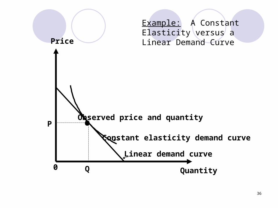
Quantity

Price

0 Q

P • Observed price and quantity

Constant elasticity demand curve

Linear demand curve

Example: A Constant Elasticity versus a Linear Demand Curve

37

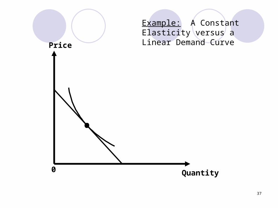
Quantity

Price

0

Example: A Constant Elasticity versus a Linear Demand Curve

•

38

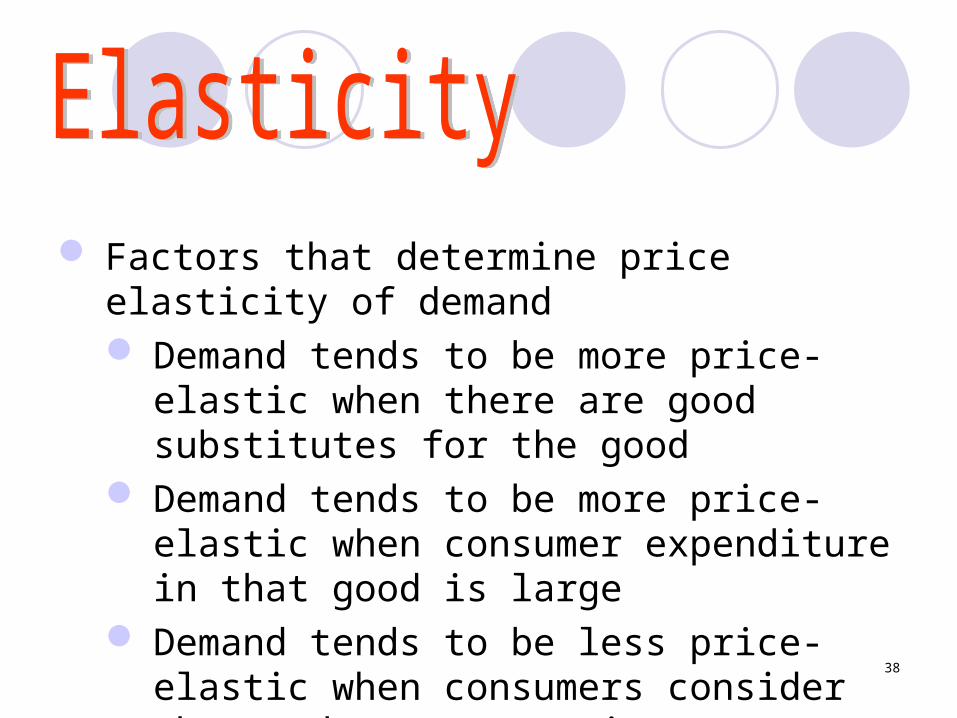
Factors that determine price elasticity of demand Demand tends to be more price-elastic

when there are good substitutes for the good

Demand tends to be more price-elastic when consumer expenditure in that good is large

Demand tends to be less price-elastic when consumers consider the good as a necessity.

39

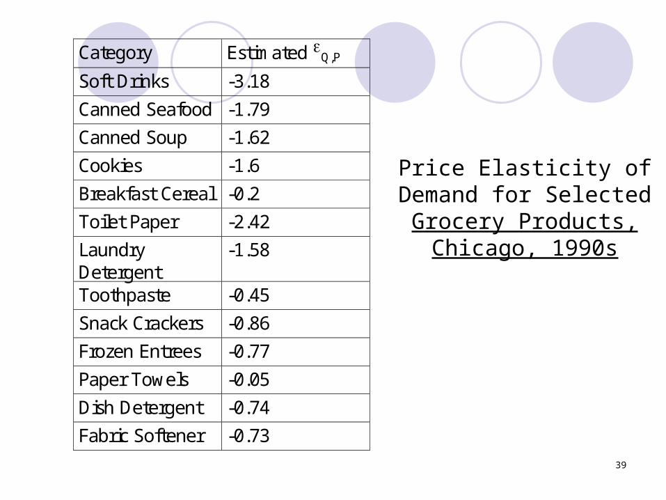
Price Elasticity of Demand for Selected

Grocery Products, Chicago, 1990s

Category Estimated Q,P

Soft Drinks -3.18

Canned Seafood -1.79

Canned Soup -1.62

Cookies -1.6

Breakfast Cereal -0.2

Toilet Paper -2.42

LaundryDetergent

-1.58

Toothpaste -0.45

Snack Crackers -0.86

Frozen Entrees -0.77

Paper Towels -0.05

Dish Detergent -0.74

Fabric Softener -0.73

40

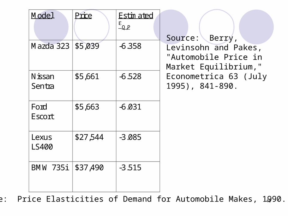
Model Price Estimated

Q,P

Mazda 323 $5,039 -6.358

NissanSentra

$5,661 -6.528

FordEscort

$5,663 -6.031

LexusLS400

$27,544 -3.085

BMW 735i $37,490 -3.515

Source: Berry, Levinsohn and Pakes, "Automobile Price in Market Equilibrium," Econometrica 63 (July 1995), 841-890.

Example: Price Elasticities of Demand for Automobile Makes, 1990.

41

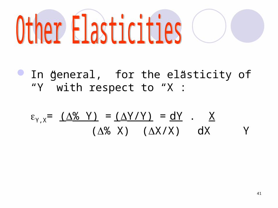
In general, for the elasticity of “Y” with respect to “X”:

Y,X= (% Y) = (Y/Y) = dY . X (% X) (X/X) dX Y

42

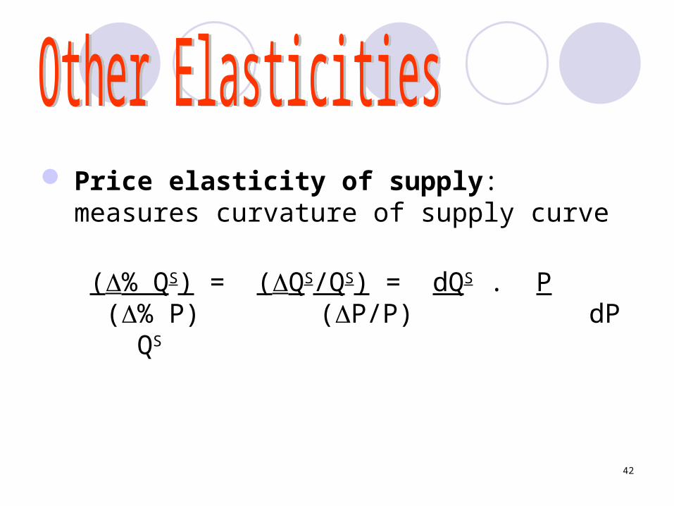
Price elasticity of supply: measures curvature of supply curve

(% QS) = (QS/QS) = dQS . P (% P) (P/P) dP QS

43

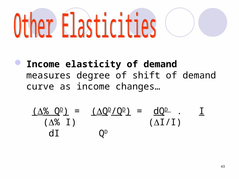
Income elasticity of demand measures degree of shift of demand curve as income changes…

(% QD) = (QD/QD) = dQD . I (% I) (I/I) dI QD

44

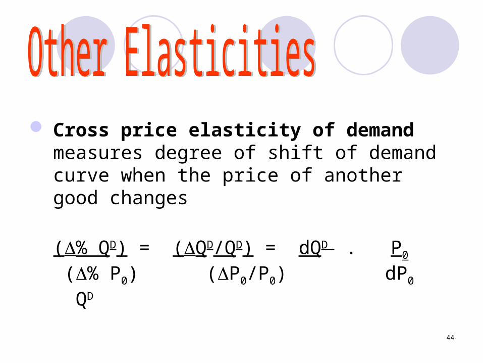
Cross price elasticity of demand measures degree of shift of demand curve when the price of another good changes

(% QD) = (QD/QD) = dQD . P0

(% P0) (P0/P0) dP0 QD

45

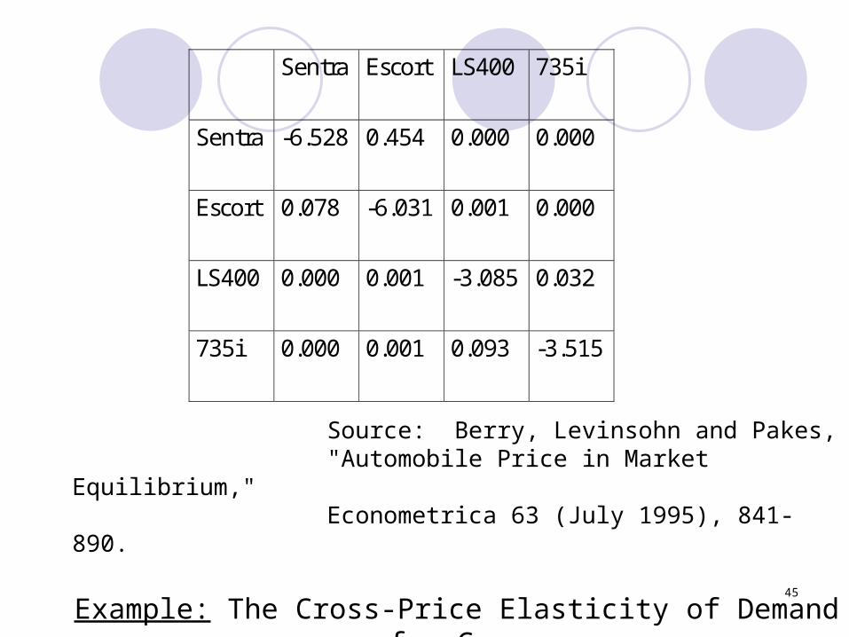
Sentra Escort LS400 735i

Sentra -6.528 0.454 0.000 0.000

Escort 0.078 -6.031 0.001 0.000

LS400 0.000 0.001 -3.085 0.032

735i 0.000 0.001 0.093 -3.515

Source: Berry, Levinsohn and Pakes,"Automobile Price in Market Equilibrium," Econometrica 63 (July 1995), 841-890.

Example: The Cross-Price Elasticity of Demand for Cars

46

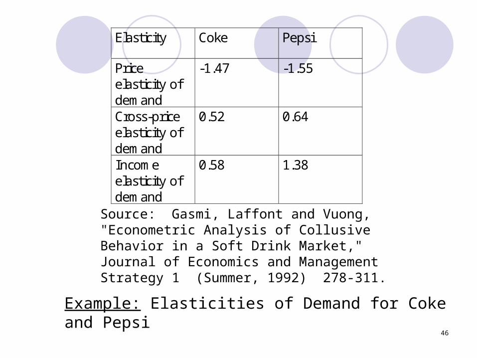
Elasticity Coke Pepsi

Priceelasticity ofdemand

-1.47 -1.55

Cross-priceelasticity ofdemand

0.52 0.64

Incomeelasticity ofdemand

0.58 1.38

Source: Gasmi, Laffont and Vuong, "Econometric Analysis of Collusive Behavior in a Soft Drink Market," Journal of Economics and Management Strategy 1 (Summer, 1992) 278-311.

Example: Elasticities of Demand for Coke and Pepsi

47

1. Use Own Price Elasticities and Equilibrium Price and Quantity

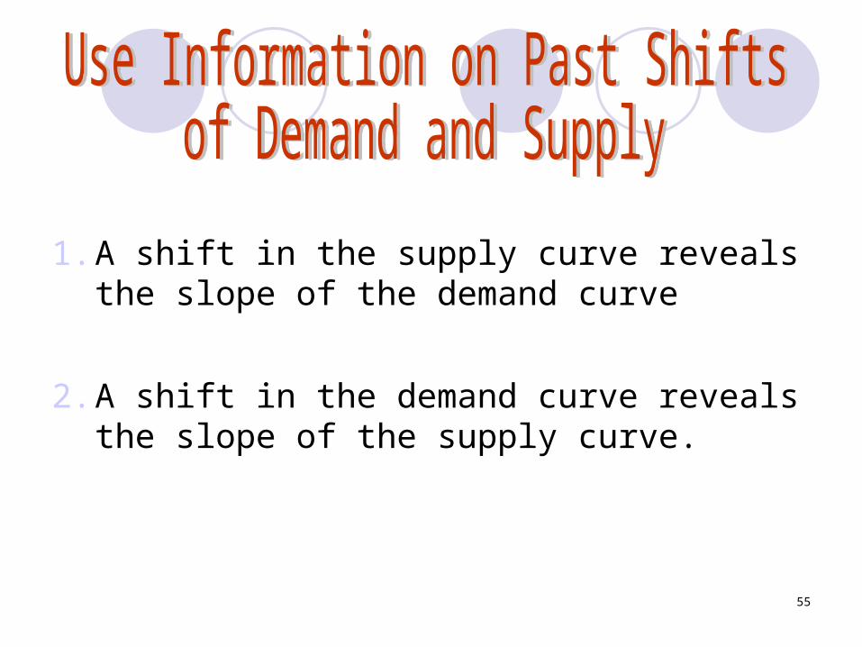
2. Use Information on Past Shifts of Demand and Supply

48

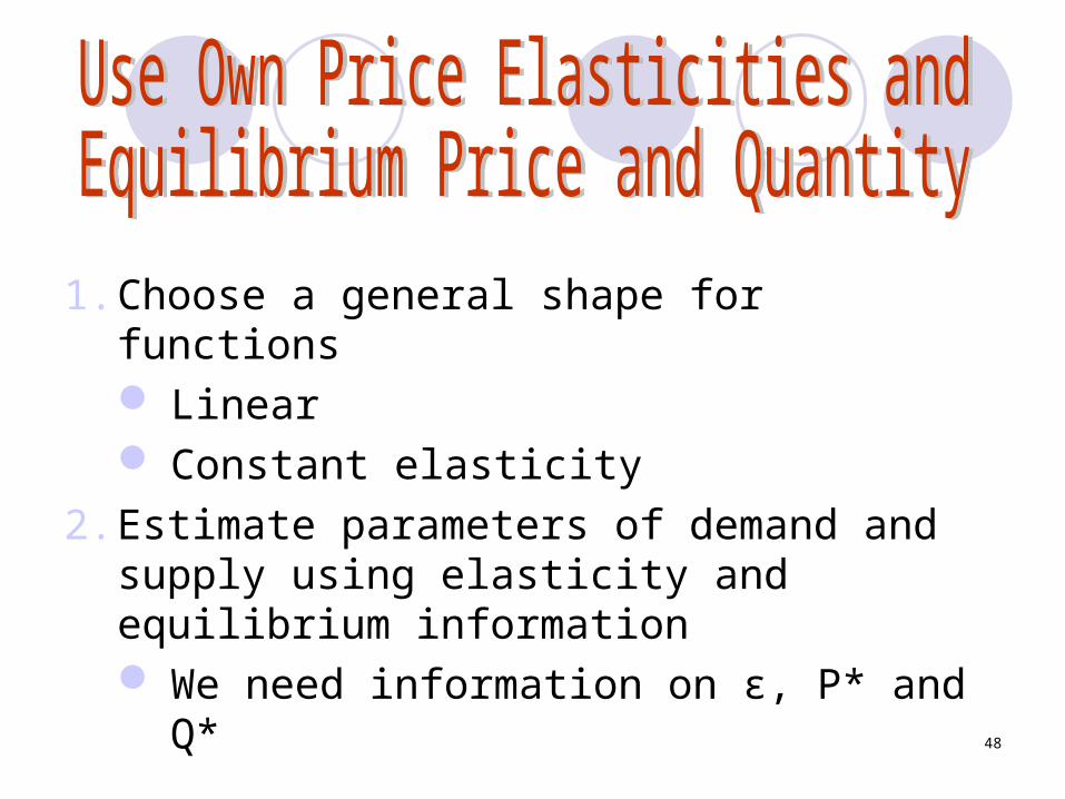
1. Choose a general shape for functions Linear Constant elasticity

2. Estimate parameters of demand and supply using elasticity and equilibrium information We need information on ε, P* and Q*

49

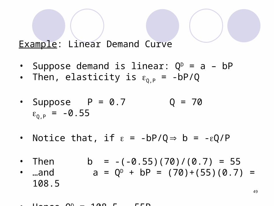
Example: Linear Demand Curve

• Suppose demand is linear: QD = a – bP• Then, elasticity is Q,P = -bP/Q

• Suppose P = 0.7 Q = 70 Q,P = -0.55

• Notice that, if = -bP/Q b = -Q/P

• Then b = -(-0.55)(70)/(0.7) = 55• …and a = QD + bP = (70)+(55)(0.7) = 108.5

• Hence QD = 108.5 – 55P

50

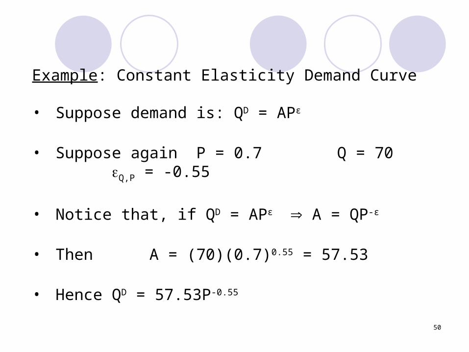
Example: Constant Elasticity Demand Curve

• Suppose demand is: QD = APε

• Suppose again P = 0.7 Q = 70 Q,P = -0.55

• Notice that, if QD = APε A = QP-ε

• Then A = (70)(0.7)0.55 = 57.53

• Hence QD = 57.53P-0.55

51

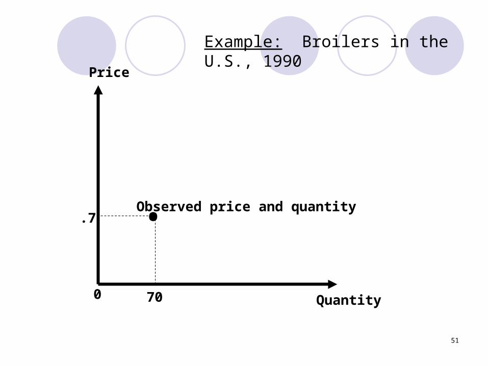
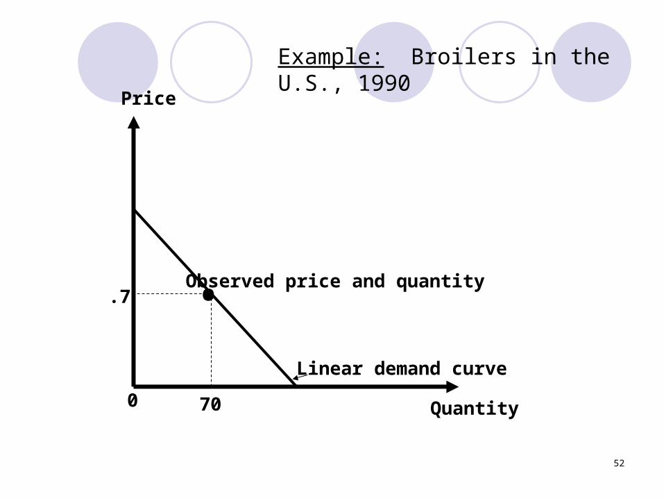
Quantity

Price

0 70

.7 • Observed price and quantity

Example: Broilers in the U.S., 1990

52

Quantity

Price

0 70

.7 • Observed price and quantity

Linear demand curve

Example: Broilers in the U.S., 1990

53

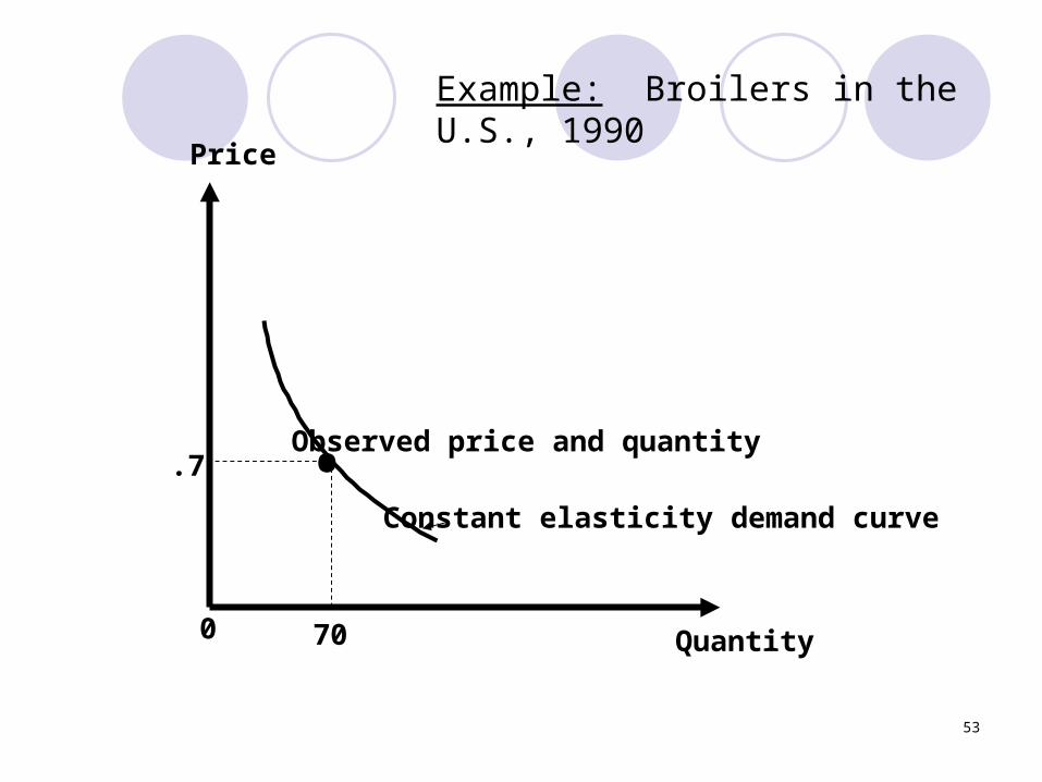
Quantity

Price

0 70

.7 • Observed price and quantity

Constant elasticity demand curve

Example: Broilers in the U.S., 1990

54

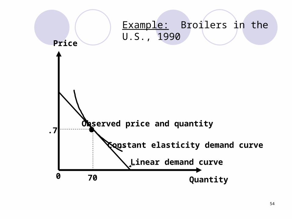
Quantity

Price

0 70

.7 • Observed price and quantity

Constant elasticity demand curve

Linear demand curve

Example: Broilers in the U.S., 1990

55

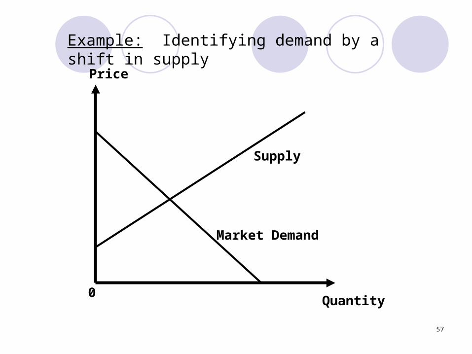
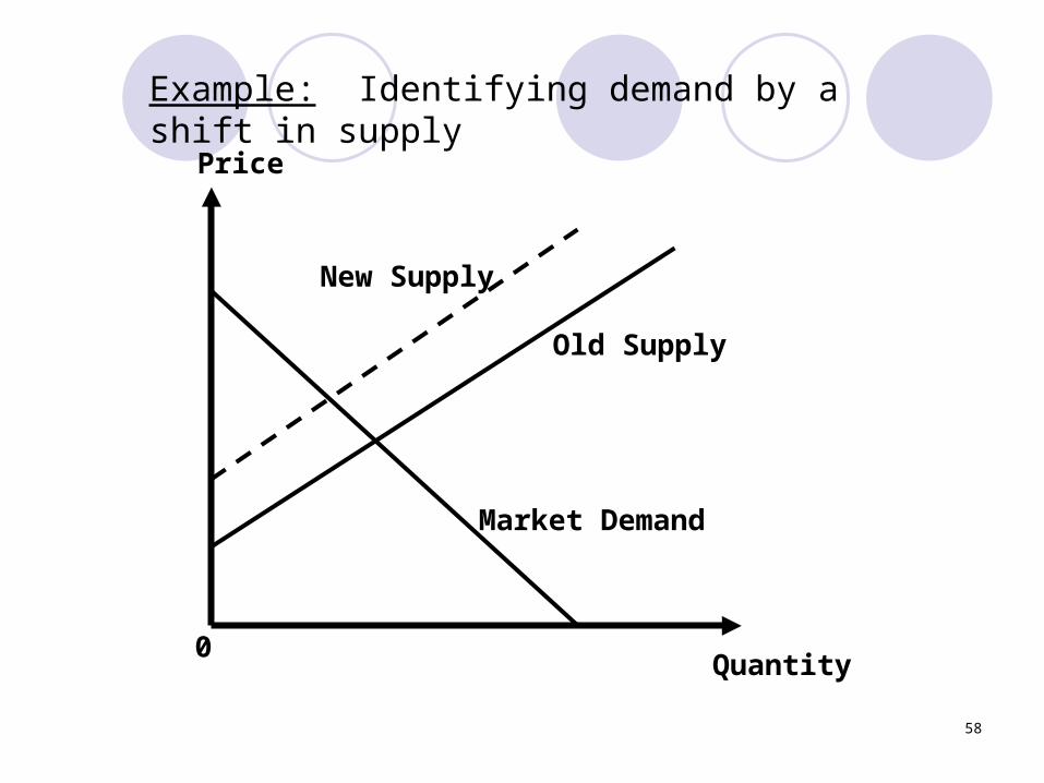
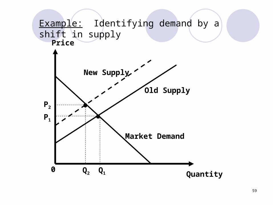
1. A shift in the supply curve reveals the slope of the demand curve

2. A shift in the demand curve reveals the slope of the supply curve.

56

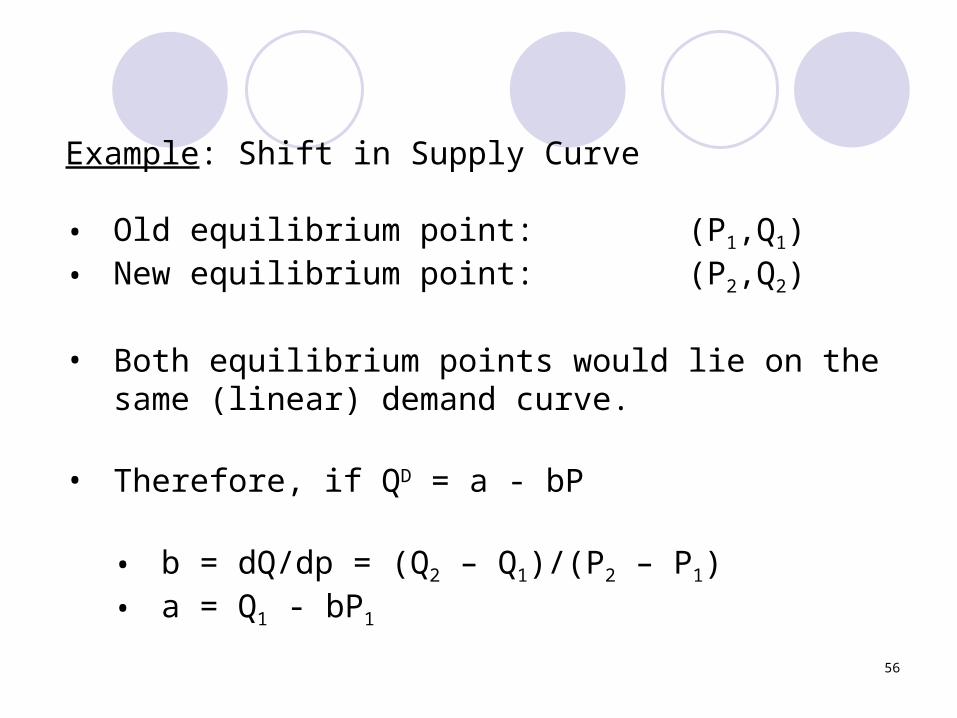
Example: Shift in Supply Curve

• Old equilibrium point: (P1,Q1)• New equilibrium point: (P2,Q2)

• Both equilibrium points would lie on the same (linear) demand curve.

• Therefore, if QD = a - bP

• b = dQ/dp = (Q2 – Q1)/(P2 – P1)• a = Q1 - bP1

57

Quantity

Price

0

Market Demand

Supply

Example: Identifying demand by a shift in supply

58

Quantity

Price

0

Market Demand

New Supply

Old Supply

Example: Identifying demand by a shift in supply

59

Quantity

Price

0

Market Demand

New Supply

Q2

••

Q1

Old Supply

P2

P1

Example: Identifying demand by a shift in supply

60

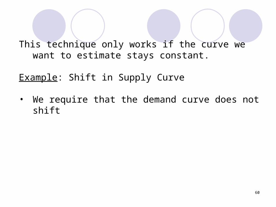
This technique only works if the curve we want to estimate stays constant.

Example: Shift in Supply Curve

• We require that the demand curve does not shift

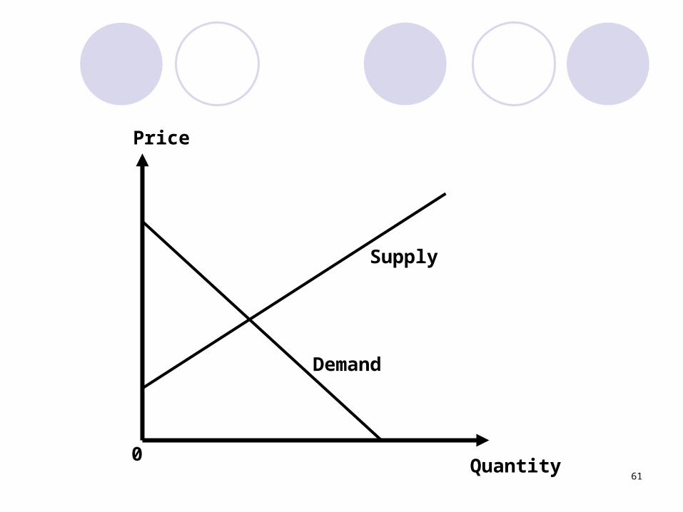
61Quantity

Price

0

Demand

Supply

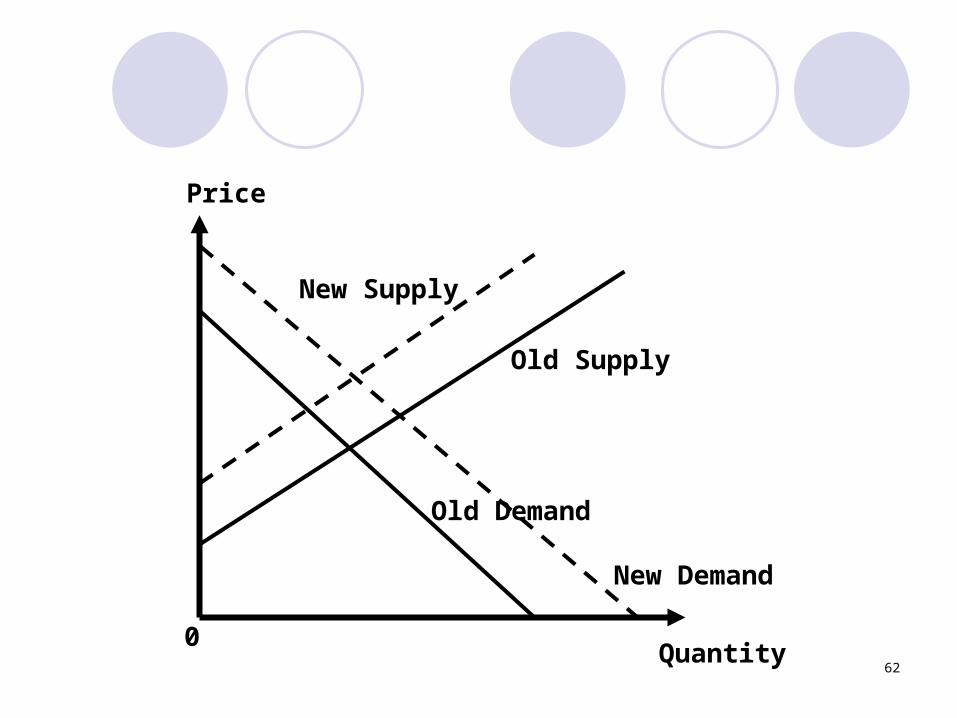
62Quantity

Price

0

Old Demand

New Supply

Old Supply

New Demand

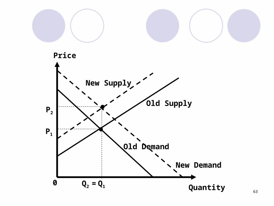
63Quantity

Price

0

Old Demand

New Supply

Q2 =

••

Q1

Old SupplyP2

P1

New Demand

64

1. First example of a simple microeconomicmodel of supply and demand (two equations and an equilibrium condition)

2. Elasticity as a way of characterizing demand and supply

3. Elasticity changes as market definitionchanges (commodity, geography, time)

65

4. Elasticity a very general concept

5. Back of the envelope calculations:

Estimating demand and supply from own price elasticity and equilibrium price and quantity

Estimating demand and supply from information on past shifts, assuming that only a single curve shifts at a time.