lec25

Performance of Marine Vehicles at Sea Prof. S. C. Misra

Prof. D. Sen Department of Ocean Engineering and Naval Architecture

Indian Institute of Technology, Kharagpur

Lecture No. # 25 Ship Motion in Regular Waves – I

(Refer Slide Time: 00:58)

Good morning, see today’s lecture is titled Ship Motion in Regular Waves. Earlier, we

have spoken about regular waves, we have followed that by irregular waves. Of course,

before I go to that, I want to speak little more on irregular sea still, which, we did last

class, but some carried over stuff I want to continue. See we mention that irregular sea is

given by what is meant a spectrum, frequency domain, energy spectrum looking like this.

Now, it turns out I was just mentioning in last class that, there are a large number of so

called theoretical spectrum available, what does it mean.

See, supposing you want to take statistics of waves in certain part of the ocean, now you

cannot do it day to day basis, people have been taking this data for years 30, 50, 100

years actually, and they have been analyzing it based on you know various time, various

year, period, geographic location, etcetera.

And it turns out that this follows they found out a Rayleigh distribution, this I mentioned

before, but the more important thing is that, there have been some theoretical spectrum;

it it turns out that you can theoretically fit some curve to find out S omega if omega is

given, which is known as theoretical spectrum, where S omega can be written as a

function of H significant T.

You can express some formulas of the spectrum, if you know significant wave height

and peak period, either you know one of them or two of them depend, there are number

of actually representation available, they call if it is only H s it is called you know single

parameter if it H s and T double parameter etcetera.

See, if you look at the literature there is a wide variety, I will only mention two of the

spectrum that is commonly used by our profession, ship building and offshore

engineering. But, basically to know that, if you knew a significant wave height, if you

knew some kind of a model period, then one can find out what the curve is, so what

happens, one goes to ocean, one has collected data and one has found out what is my

significant wave height based on some you know observations, some calculation.


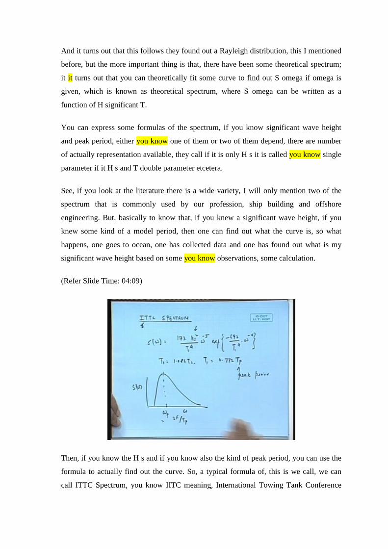
Then, if you know the H s and if you know also the kind of peak period, you can use the

formula to actually find out the curve. So, a typical formula of, this is we call, we can

call ITTC Spectrum, you know IITC meaning, International Towing Tank Conference

Spectrum. A two parameter spectrum, this is most commonly used, because this is

supposed to represent an average sea all over the world.

See mostly when we do a ship what happens is that, the ship is mostly for ocean going all

over the world. So, it must represent some kind of a, it must I mean be able to travel in in

a wave which by description is an average kind of wave for all over the world, global

wave, not you know a typical wave happening in one place this is best represented by the

spectrum. The formula for that is given as S omega equal to some, I do not remember

where if I give this formula last class, then T 1 is some kind of a period, see T 1 seem

turns out to be some period or T 1 equal to 0.772 T p, this is called peak period.

What it means is that see, if you knew H s and if you knew T p, you can find out what is

S omega for various omega, it will turn out to be something like that, this is actually

where the peak occurs, this is omega, so this is my, you can call omega peak which is

equal to 2 pi by T peak this is S omega. So, in other words if you knew H s and if you

knew T p, you can find out this the frequency distribution of the wave, this is a typical

ITTC Spectrum, this looks like that.


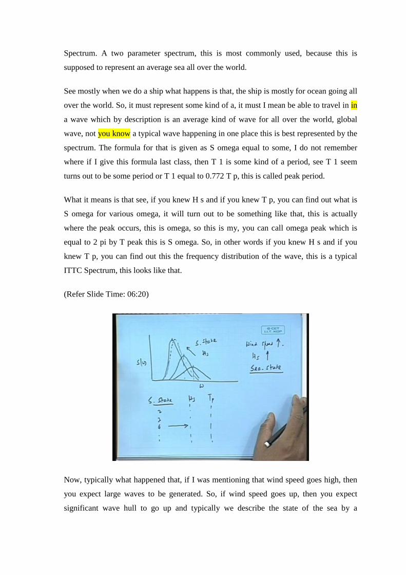
Now, typically what happened that, if I was mentioning that wind speed goes high, then

you expect large waves to be generated. So, if wind speed goes up, then you expect

significant wave hull to go up and typically we describe the state of the sea by a

parameter called Sea-State, this is not very well defined, but you know you use the what

sea state 1, 2, 3, 4, 5.

So, something like sea state say 2, 3 like that goes, it will imply H s equal to some ranges

it will imply T p is some ranges. There are some ranges there that, if you say the ship

should be capable of operating in up to sea state 4, that would imply that going to the

table that it must be able to cater to significant wave height of so much of T p so much.

Now, typically what happened, lower sea state waves spectrum look like that as the sea

state goes up it looks more like that; this is actually, this is lower sea state as the sea state

goes up, the sea goes like this or as H s goes up it goes like this. What it means, when the

wind is low you expect low energy, so the area under that is low, because area under that

represent that significant wave height, it is less. What is more important is that, you

expect waves of smaller length to be excited more, so it is spread like that, see this is this

wave length is smaller than this wave length, because wave length is inverse proportional

to 1 by root over of frequency.

Now, as the wind speed peaks up, significant waves goes up and it goes like this. So, the

this this spectrum has this peak period also, because sometime it happened that

depending on the location, you can have another spectrum of same area, but having a

peak may be slightly different. This is why you know in single parameter spectrum

which has only H s, which will not a differentiator between the two, but in this two

parameter it fixes this point as well as the area under that, this is one of the most

commonly used representation.

Let us say, let me put it in more simple terms as far as we are concerned as a user, we do

not worry about how oceanographers have collected the data; we assume that they have

collected the data that they are given as a spectrum, and our job would be to use in

appropriate spectrum and then tell that look my ship should be capable of operating in up

to sea state 3 or 4 or 5 this is a typical spectrum.


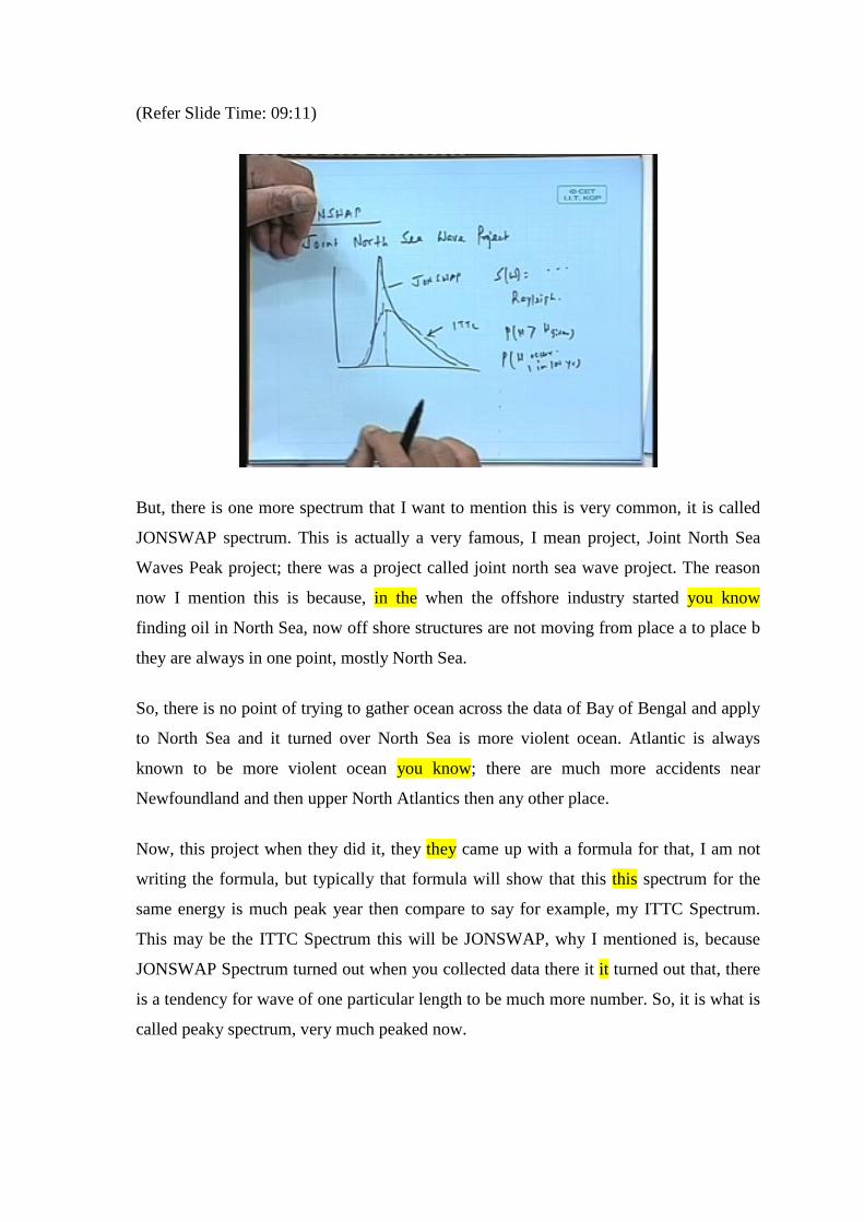
But, there is one more spectrum that I want to mention this is very common, it is called

JONSWAP spectrum. This is actually a very famous, I mean project, Joint North Sea

Waves Peak project; there was a project called joint north sea wave project. The reason

now I mention this is because, in the when the offshore industry started you know

finding oil in North Sea, now off shore structures are not moving from place a to place b

they are always in one point, mostly North Sea.

So, there is no point of trying to gather ocean across the data of Bay of Bengal and apply

to North Sea and it turned over North Sea is more violent ocean. Atlantic is always

known to be more violent ocean you know; there are much more accidents near

Newfoundland and then upper North Atlantics then any other place.

Now, this project when they did it, they they came up with a formula for that, I am not

writing the formula, but typically that formula will show that this this spectrum for the

same energy is much peak year then compare to say for example, my ITTC Spectrum.

This may be the ITTC Spectrum this will be JONSWAP, why I mentioned is, because

JONSWAP Spectrum turned out when you collected data there it it turned out that, there

is a tendency for wave of one particular length to be much more number. So, it is what is

called peaky spectrum, very much peaked now.

See in this one ITTC Spectrum, energy of waves of this frequency and this frequency it

is maximum no doubt, but it is somewhat spread. But in this one, you have got much

more waves of only at that particular height, why it becomes important, we will see

afterwards that if you have a structure which actually behaves badly in this wave, then

obviously it is going to be a very badly JONSWAP Spectrum, that we will discuss when

we talk about ship behavior in waves.

I just want to mention this because of its historic importance this JONSWAP Spectrum,

the second point is that now that, I know S w by a formula this is a Rayleigh distribution.

It turns out that if so, you can find out every possible statistical property based on this S

w equation you can find out.

Number one, what is the probability of wave height exceeding so and so, what is the

probability of a given wave height, probability of say H exceeding certain given, what is

probability of H occurring once in 1 in 100 years this is too small, but you can just note

my word.

You can find out every possible statistical parameter like chances of wave not occurring

less than this more than that period so and so, what is the chance of a return cycle of a

give wave; that means, after how many cycles statistically one particular height will

repeat, what is the maximum height expected in 30 years, what is the maximum expected

in 100 years. Everything can be found out form this formula, if you assume that to be a

Rayleigh distribution in all statistical property becomes available, this is what we do.

Therefore, see things becomes simple from our point, if we can get an H s significant

height and T p for a sea state for a given sea state I go to H s and T p, then I go to the I

choose appropriate spectrum formula once I choose that I can find out every parameter

what is the chance of you know a wave height exceeding so and so.

Afterwards we will see that what we will want is not the wave height exceeding so and

so, but perhaps what is the response exceeding so and so. Wave height is also important,

because suppose I find out as an example an offshore structure I find out that the chances

of a wave height exceeding no, the chances of maximum wave height occurring once in

100 years is equal to say 20 meter.

Then obviously, what I will do I will design the structure, so that it can survive up to 20

meter high wave. You see, this is how the statistics come; you cannot design for infinite

time you have to go statistically. So, there is statistically a probability of what they called

return cycle. So, suppose once in 100 years means, you can break it in seconds and if the

wave is 10 second, so you know that after so many cycles this wave’s case repeated.

So, let us not go into that detail, because we do not have so much time, but just the point

is important that all statistical properties, everything that you may want to know ever, for

design becomes known. This is a short term statics there is one more thing I should

mention here, what is called long term statistics.


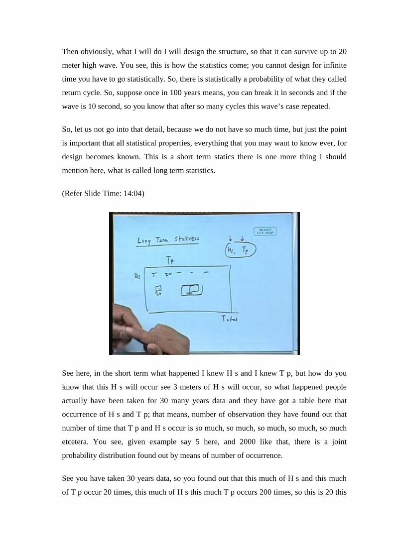
See here, in the short term what happened I knew H s and I knew T p, but how do you

know that this H s will occur see 3 meters of H s will occur, so what happened people

actually have been taken for 30 many years data and they have got a table here that

occurrence of H s and T p; that means, number of observation they have found out that

number of time that T p and H s occur is so much, so much, so much, so much, so much

etcetera. You see, given example say 5 here, and 2000 like that, there is a joint

probability distribution found out by means of number of occurrence.

See you have taken 30 years data, so you found out that this much of H s and this much

of T p occur 20 times, this much of H s this much T p occurs 200 times, so this is 20 this

is 500. So, there is a table full of numbers simply telling the number of time this

significant wave height has occurred in a given location.

Now, tomorrow therefore, you can find out what is the chance of, my this H s occurring

because, I have got an out total observation, say total may be in order of 100000 of

which you found out that 5000 has occurred to observation with H s between 4 to 5

meter. Therefore, the probability that H s will occur 4 to 5 meters is 5000 by 100000.

So now what happened, the chances that as ship is going to encounter a wave of H s five

you know 4 to 5 meter is going to be that much percentage. See, suppose I design a ship

which withstands obviously, I will investigate how it behaves in 1 meter height wave, 2

meter height wave etcetera, but then it is not always meeting 10 meter high wave, it is

meeting 10 meter high wave say significant high wave may be 2 percent of this time 5

meter may be 20 percent.

So, this is called what is called a long term statistics, in a long term I can, see earlier

given H s given T p I find out what is the chance of this exceeding something, but here I

am going long term. I am trying to find out what is the in 30 years chances of percentage

of time H s may occur, you get my point now, this is just to give you a brief idea, this is

how the oceanographers go.

See let me give you an example, we are designing a ship to go from here to, let us say

Singapore, so it goes to a certain sea and let us say I have data for that particular sea.

Now, I find out that in that sea chances of H s occurring 8 meter and more is only 2

percent, 6 meter to 8 meter is may be 20 percent, 4 to this is so many percent; now, for

each one I will find out see for 8 meter is certain percentage, 6 to 8 is certain percent,

now for each one I find out what is my response say roll if this, if 8 meter wave occurs

my roll becomes a 15 degree see if this occurs my roll make 10 degree.

So I now know that 15 degree of roll may occur so many percentage of time 10 degree,

may occur, so many percentage of time. So, I can find out what is my total probability of

certain roll occurring, response occurring yes, this is the idea because there are two way

therefore, the probability one is that given time the waves are continuously changing, so

I get H s, but then I have taken the data today for 2 hours, so I found H s from the

irregular sea, but I took it last year I took it the previous year so now, I find out from

each one what is the chance of H s so and so occurring.

So, you know it is a it is say, so you can imagine this is where the oceanographer come

in, oceanographic it is a huge amount of data, each point long data. You have to do it for

many times, many years, and statistically analyze all we need to do is that we have to

find out in a given ocean what is the chance that the ship will not exceed or will be

within certain operation limit.

Because from that, you can figure out suppose you say that the ship roll exceeds 10

degrees and you say that if it exceed 10 degree, you cannot do an operation. So, you can

find out the down time in offshore structure if it, heave is more than certain time says

four meter then it cannot operate. So, you find out that the chances in this sea, in a long

term that the heave will exceed 4 meter is equal to 20 percent. So, you say I have 80

percent you know operation time, 20 percent down time like that we go.


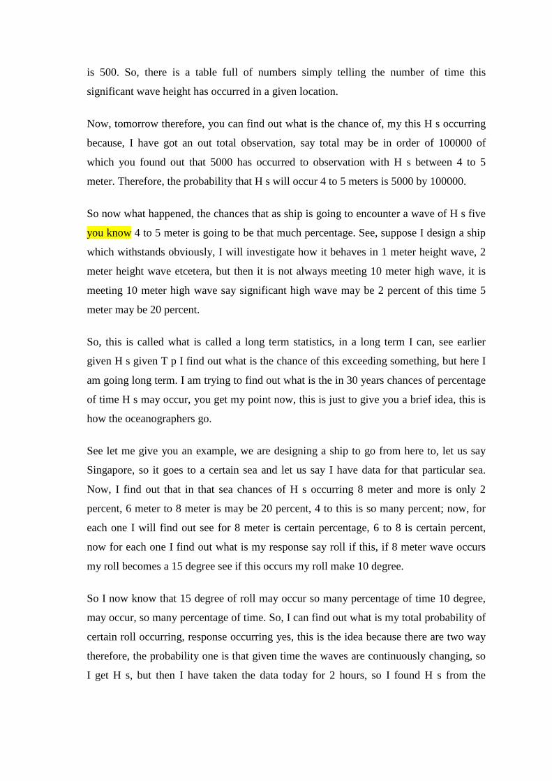
Last small thing, that I want to mention is that in this case I took all the waves coming

from the spectrum one side, all this we have added together to find out the spectrum.

This is what we call 2 D or long long crested sea, because what happened in here, if you

stand here I mean in a this thing, this waves are crest is long along the x axis I mean the

waves are going this, all of them are go in one direction.

So, on the crosswise y direction the crest is continuously long, because here that the

spectrum was based on the assumption that we have done in the previous class, we have

added all the waves, but all the waves that we are added were all in the same direction.

But, in reality waves can come from this direction, can this direction, can this direction,

can this direction (Refer Slide Time 19.22). So, now if you make a more complex

picture; that means, if you want to say that the wave that I have got at point a is not only

because of all waves coming from direction one, but also from all waves from direction 2

and 3 and 4 and 5 and 6.

So, in other words if I assume that a particular point the waves that are coming are all

waves in one direction all omegas, but also all omegas from all thetas. So, it becomes a

more complex analysis; that means, you also find out the directional spreading.


So, what happens you see it is goes something like that, that you assume that supposing

all waves came from one side it would be like this, spectrum would become like that, but

now this when all the waves are coming from this direction, but if all the waves are

coming from this direction, all the wave come from this direction etcetera, it will be

something else. Here, what we do you assume that as if some waves are coming from

this direction, some of the energies because of waves coming from this direction, some

from this direction, some from this direction.

So, you can imagine that it is something like, this curve is being rotated like a bell curve,

like this curve will be rotated here, rotated here it is difficult to.

This axis will change

Yeah. So, it is like a graph we are use as rotating it, but you see if the now now, there is

an interesting point suppose wind blows this side, you would expect most waves to be on

this side, but you will also expect waves from the other side, but to an less extent

ultimately you will expect almost 0 waves from 90 degree angle. So, this is how this idea

of, what is called 3 D or they call short crested sea or short crested spectrum; where what

they do is that what we assume is that look. The energy of all the waves are not only

coming from direction one, but form all direction; however, the directional spread this is

called spread is diminishing from the main direction and it will go to 0 as we go down.

So, typically what they do is S 3 D omega is written as S 2 D omega into this is actually

omega and theta because, it is it is the function of both into one spreading function.

Typically, what we represent is that we say that the three-dimensional sea is two-

dimensional sea multiplied by a spreading; that means, there is a two-dimensional sea

when theta equal to 0, some value theta equal to 10 degree, some other value and as it

goes to 90 degree it becomes 0, so f theta becomes what this is called, spreading function

given example of the spreading function.


Now, here f theta one of the typical f theta value is for example, 2 by pi cos square theta,

if you see that, you will see that f theta becomes 0, as theta becomes 90 degree. And if

you integrate f theta d theta over this angles actually minus pi by 2 plus pi by 2 this will

become plus 1.

So, what this is very interesting because what happens see S 3 D, I will I will very briefly

tell this S omega into f theta, see remember that area under that, see area under this, area

under see now this is my spectrum, so if I integrate that, and integrate that, and integrate

that, what happened this represent area under the spectrum (Refer Slide Time 22.57).

Now, the area under the spectrum represents the total energy that has been transformed

to the wind. So, the energy is constant now see the entire energy might have gone to

produce waves only in direction 1. But you can also assume that, look this entire energy

spread some part of it is actually producing waves in direction 1 and another part is in

direction 2 etcetera.

So, integration of this which represents energy always must remain constant, so this must

be equal to this, but then this is I have done where also represents the energy, same as the

2 D spectrum. So, this integration must be equal to 1, see then this condition gets

satisfied this is the basic philosophy actually, what I am trying to say I will I will give an

example numerically will be easier; say let us say this energy is equal to 100 unit, now

this the total energy is 100 unit of waves.

So, now supposing I assumed all these energies coming from direction 1, then my two-

dimensional thing would have been 100 unit, but what we do is that, we say this 100 unit

is spread there is 100 unit this would be hundred unit coming all waves in this direction.

But I am going to say that this is equivalent to 80 coming from here, say 60 coming from

here say, 20 coming from here, 5 coming from here, 2 here like that, so that the sum of

this 60, 20, 5, 2 etcetera will become equal to 100 this is called directional spreading

(Refer Slide Time 24.17). Now by doing this formula, we find out an S theta where this

sum becomes remains 100 I give better example of of this here, see this book.


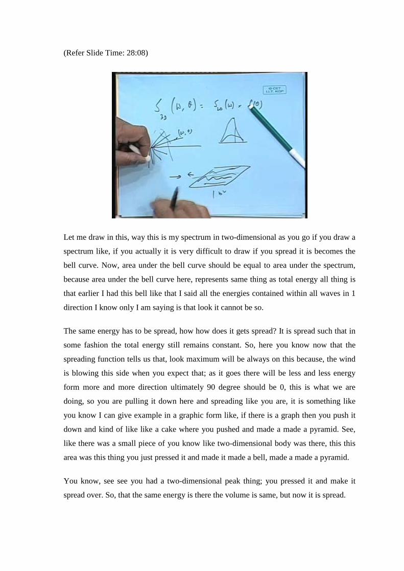
Let me draw in this, way this is my spectrum in two-dimensional as you go if you draw a

spectrum like, if you actually it is very difficult to draw if you spread it is becomes the

bell curve. Now, area under the bell curve should be equal to area under the spectrum,

because area under the bell curve here, represents same thing as total energy all thing is

that earlier I had this bell like that I said all the energies contained within all waves in 1

direction I know only I am saying is that look it cannot be so.

The same energy has to be spread, how how does it gets spread? It is spread such that in

some fashion the total energy still remains constant. So, here you know now that the

spreading function tells us that, look maximum will be always on this because, the wind

is blowing this side when you expect that; as it goes there will be less and less energy

form more and more direction ultimately 90 degree should be 0, this is what we are

doing, so you are pulling it down here and spreading like you are, it is something like

you know I can give example in a graphic form like, if there is a graph then you push it

down and kind of like like a cake where you pushed and made a made a pyramid. See,

like there was a small piece of you know like two-dimensional body was there, this this

area was this thing you just pressed it and made it made a bell, made a made a pyramid.

You know, see see you had a two-dimensional peak thing; you pressed it and make it

spread over. So, that the same energy is there the volume is same, but now it is spread.

Spread is.

And the as you go away from the main directions; obviously, the energy is less

ultimately 90 degree it is less 0, because see if the wind blows from this side you do not

expect any wave form this side. So, maximum wave will come from this side, little less

here, little less here, little less here, ultimately 0 here and no waves of course, coming

from this side, because winds are in this way (Refer Slide Time: 26:32) When you have

this representation this is what is called a short crested sea. Because when you the reason

I mentioned that is that again therefore, it has become algebra S 3 D becomes simply S 2

D into f theta.

Now, this is depends on, this depends on only H s and T this is only theta. So, you see

although when you have gone to open ocean you find out waves are all kind of irregular

and there are no crest, there it is all you know random the full thing can be nicely

represented by knowing only the significant height peak period and spread function

which is known.

So, although it is very confusing as I said even the two-dimensional is confusing 3 D is

even more, but it can be broken down to nice comprehensible the easy algebra. This is

what I want to say here as far as the wave is concerned a 3 D part.

This is very simple if you want apply, what happened in the what they call confused or

irregular sea actually I am fond of saying that, this is the list confusing part if you keep,

if you once we get in the class that the algebra straight, it is pure algebra there is no

knowledge just algebraic breaking down.

Sir, 3 D part is just moving part for this is one and theta also comes

Yeah yeah see it is may see S 3 D has a function of omega into theta, because it will

depend now see the value of this will depend on any omega and any theta. Because you

see it is it is a it is a bell curve, so you have got a bell there is a line here, there is a line

here, line here, line here, line here it has got it is a bell, so everyone you know like like a,

like a, at every (Refer Slide Time 28.17).

Pointer

Omega and theta you have a value, up value; this is like that how to find out that value,

that is found out by taking S 2 D into omega multiply f into theta. So, for that given

omega you know H 2 D that, that is actually the bell curve that original bell curve. But

multiply that by an f theta; that means, you you are lowering it down actually see f theta

will be actually a function which will obviously, become as theta goes to 90 degree

becomes 0. So, it just a number, so you are just as if you are pulling this down as if this

graph is pull down as you are spreading it.

If you see the picture is very simple actually there is a you know this is video class we

have problem of showing this demo, you have this line here you know, this line is here, I

as spare it and pull it down see I have, I will show you here this this is my spectrum here

as I shift it I just push it down like that, that is all. I mean I have a graph here, I pull it

down and spread it and as 90 degree it has become 0 and now this graph that I have got

exactly having the same area as the first graph. So, meaning that the energy of the wave

is exactly same.

So, it is something like I have an open ocean this is 1 meter square area. So, all kind of

waves are there, I know that the energy of that must be constant. Either now I can think

is all the waves are coming one side, but I can say the same energy spread are shared by

waves from all directions; this is what I have done. First place I say that all the energy

shared by all waves from 1 side, but now I say all the energies shared by always from all

sides.

However sides are having a bias, because you would expect more waves from the side

wind is blowing this waves from other side, you know you cannot expect there wave

coming from this side as well as from this side, because opposite side will you know

cancel each other.

So, I think this is way I am going to end so called my description of irregular sea. So,

what we have done is regular sea description, irregular sea description, regular sea was a

simple sin curve, irregular sea is nothing but some of those sin curves, that is all now

what we have to know is coming to the more topic.


Now, we have to bring the ship in and put in the ocean. So, obviously the first step is in

regular wave and in fact, we will find out that this is the the most difficult task. So, I

have got now a sin wave coming, I have got a ship here I just want to know how it moves

up and down, wave of period say 10 second with height 5 meter, I want to know how

much the ship would responding, if I can find out later on I can say that a spectrum is

nothing but so many waves, so I can also add the response like that, that is not simple

part. So, before going to that, now we need to know first define the ship motion, the first

thing would be definitions; this it it appears very simple to all I tell you, it is not always

that simple, because what we know layman it is I mean you know layman’s term is fine,

but there are some assumption inherent to that which we do not tell.


Say now, let us say we take a ship here, I am just falling this book here, we are going to

use this kind of you know say x body here, say y body here, this is z, this is may be g

here, center of gravity here. See, everybody knows I mean, I am just showing a ship here

with some axis, we can say it is typically when you read hydrostatics and all we have a

fixed axis along the length direction.

There is longitudinal axis x b on the body you know transverse axis y b and z b I am

calling it, that is a an axis of the body obviously, everybody knows that the linear motion

here is called surge, this is called sway, this is you know up and down motion, this is up

and down motion, this up and down motion, is called heave, that I think all of us know.

Then this is see x 1 many ways are putting, I can say this will be axis 1, axis 2, axis 3,

then along 1, 2, 3 is surge sway heave, now about one that is this motion is roll then, this

one is pitching and this one is yaw.

So, you can say surge, sway you got linear, along x b, y b, z b and roll pitch, and yaw is

angular motion about same three axis, x b, y b, z b. So, there are three, now we we we

are using right handed coordinate system, remember that angular motion means when I

say about x b that is clock wise direction; that is you know this way if you axis is there,

this this axis is there means going like clockwise direction. You have to remember that

because otherwise, in the calculation we have make mistakes you know that axis.

Therefore, it is here means, this way here, means this way; that means, you see bow

down is pitch positive in this and here, it is this I mean going on the what you call port

site is a positive yaw and then, this is but this is very simple all of you know that, but

now there is a problem.

Problem is that when I want to observe the ship from a fixed axis I am on a shore, this is

not this x this x b, y b, z b continuously changes; what happened in a let me give an

example in a wave the ship is at this movement like this, so my x b is this side, z b is this

side, so should I call this this motion heave or should I call the vertical motion heave. So,

the question comes of the axis you see I mean this one I want to say this one very clearly

if you use.


Suppose at some point the ship is like this, at some point of time now, my x b was this

way; my z b is this way, so is is this heave, if this is heave next instance that ship is like

that then next instance, if this is going to be heave. So, the heave direction will keep

changing say today, you call this heave tomorrow this is heave every instance the heave

direction change roll also same thing. So, you understand this is an important point we

have to understand at the beginning, because we already said ship is heaving 4 meter

which is the axis.

If you say the axis what I defined as a body fixed axis, the body is changing

continuously, so my horizontal is changing. Take a submarine it can dive here like that,

so will you call this to be heave or the vertical to be heave right.

The axis are fixed to the body then

That is ok

Even then, no, ok fine, axis fixed to the body there is a ship here, it is the submarine is

diving like that; axis is fixed to the body this x as this z. You are calling the motion along

z axis is to be heave will you call now this is my vertical remember, this is my water

water surface will you call this to be heave.

But inside the angle

Yeah, but will you call this heave when you say the ship is heaving.

I will select the reference.

You see, that if you call it heave the next instance the ship is changed this direction. So,

that the motion.

Company will surge and heave.

No no, when you say the ship is heaving 4 meter, what do you mean it is see, in this case

the heave axis is continuously changing to this side, this side, this side, this side like that

going, so which one is you call heave, when you say 4 meter is on, this 4 meter, because

it is not fixed here it is continuously changing.


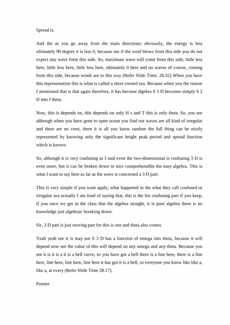
See, unless when you saying roll also, roll you say above this axis, but you know the ship

may be actually, always at about some you know it it may be actually like this position

and then rolling some angle or it can be actually above this position then having 10

degree, they are not same specially pitch is not same thing; especially pitch in a typically

say submarine kind of case you know will you call, I mean these to be pitch or this to be

I mean the ambiguity will come which is the axis you want.

Let us taken simple case, you would want the motion along the vertical axis to be heave,

let us because, heave is more commonly known, but if you fix along the ship axis then it

is not that the z motion z b is not always vertical it is changing.

So, therefore, we need to have some more generalization of definition it is not safe;

second thing is I can tell you the axis supposing I put this is an axis, and I put this this

thing and tomorrow you decide to put this is an axis you know I will take another

column.

Now, you see this is my one axis, this is my another axis, now if you define motion

above this axis and rotation above this axis that is heave, pitch, roll etcetera. And he

decides that I am going to be use this two will axis, will you get a same roll when you

say 10 degree roll he is thinking that it is rolling above these axis going through these are

I am thinking its above these axis. So, again there is ambiguity you have to first, define

the axis then define that I am going to tell about this axis this motion is roll pitch here.

Roll pitch.

So, you cannot say just you know in, I am taking in a very strict sense, we will find out

that when the motions are small the distinction is not there, but if you want you know

from the beginning every strict sense you have to first define the axis, origin of the axis

then tell that above these axis, this motion I am going to call heave, roll and pitch.


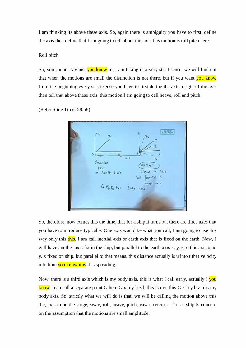
So, therefore, now comes this the time, that for a ship it turns out there are three axes that

you have to introduce typically. One axis would be what you call, I am going to use this

way only this this, I am call inertial axis or earth axis that is fixed on the earth. Now, I

will have another axis fix in the ship, but parallel to the earth axis x, y, z, o this axis o, x,

y, z fixed on ship, but parallel to that means, this distance actually is u into t that velocity

into time you know it is it is spreading.

Now, there is a third axis which is my body axis, this is what I call early, actually I you

know I can call a separate point G here G x b y b z b this is my, this G x b y b z b is my

body axis. So, strictly what we will do is that, we will be calling the motion above this

the, axis to be the surge, sway, roll, heave, pitch, yaw etcetera, as for as ship is concern

on the assumption that the motions are small amplitude.

This is what we have, see that the debate can go on for a long time, because it turns out it

is not very simple, but for all definition it turns out that is suppose now, motions are very

small then the difference between x b, y b, z b and x, y, z becomes what is call I you

know I I am fond of using the word too small. You know like small into small makes it

too small, is very small, too small what is called second order quantity, so the difference

between the two deminicious, if you are assuming that the motions are of small

amplitude.


In other words, I will write if between o x b sorry, x b y b z b and x y z is too small,

actually you know epsilon into epsilon it is order of what you know mathematically it is

what is called, it is a second order quantity you know, if there is a small thing that, if I

have the small into another small makes it small square see point 01 into point 01 makes

it very small you know like that.

We need not worry about that, but if you want if somebody wants very rigorously

mathematical the consistent then it one can explain. Now, we will define for us the

motions sorry x y z; that means, it is above then axis which is fixed on the ship, but not

rotating just transferring; that means, it is see the ship is like that, but the axis remains

like this, ship is like that but the axis remains like this, the axis is going with the ship, but

not fixed on the ship, axis origin only its fixed on the ship, only the G point is fixed on

the ship .

Again there the origin now most convention, earlier there was two things one was to use

see this is water line here, this is water line you know earlier these people were using is

this G here, some people use to use a point just above LCG, but at the water line level

this o as origin that was the old convention, but now a days it is more conventional to use

G as the origin.

But units parallel with the water wave


Yeah parallel with the water wave, if this diagram again I will draw little bigger see now,

convention wise this is the ship here let us say this water line fish at the part, so you

know that this is water and here. So, here some people use to use this is LCG, G point at

one time this was used as the origin, but that was more earlier literature now a days it is

more convention to use, this as origin, both can be calculated, but you see the question is

that normally the difference between the two, because this distance is small will not be

very small.

So, there are programs where you can calculate the motion based on this or based on this

there will be some extra terms coming; however, that is not the point you can calculate,

but the results that you produce should be specified with respect to the axis. Because you

first you will say that look I have taken G as an axis and based on that my motions is this

degree, that degree, that degree.

People do not say that reason reason is because, the differences are too small especially

practical people you will never tells some hear, some what is saying G and all its a ship

rolls 10 degrees that is all is not it I mean people will say ship is rolling badly or it is

heaving badly, that is what we will tell because, the distinction the difference between

this this becomes very small in practical.

See where you take given example, this case we took all always like this, but we did not

understand that actually if you want to do that the ship you know it was not here, but it

was somewhere here therefore, the ship have to be have actually pushed up. So, when it

rolled it it automatically underwent and heave.

And when you dig that you see about which point I rotated, I do not know if I rotate

about this point, then the ship orientation look something else. If I rotate about this point

the orientation will have something see a simple example, if I rotate about this point the

ship would look like that if I rotate about, this point it would look something else see it

would look something like this, is it not?

So, its location in space actually differ depending on about which point you will, you are

sort of turning; however, what happened in both cases see the angle is 10 degree. So,

normally we say that it has heave 10 degree, but if you want to see the complete story it

has heave 10 degree also pitch so and so, because I want to find out in way, where it

exactly it is, what space it occupies that does not become unique.

So, if you want to numerical simulate, say you have a simulator then you know if you do

not say the axis it will give you 10 degree roll, but it may not be the exact location where

it is suppose to be. So, in one case you may see that that you know a side say bank

another case depending on that you do not see it. So, what I am trying to say in short is

that, the the space that a ship occupies you know in space or the place that it occupies in

space you know, exactly see this is a D 3 space, where it is exactly located with respect

to a frame that will depend on about which axis you are rotating.

See, I can rotate 10 degree here, but I can also get that 10 degree here, but these two are

not same. So, if you want to be very exact that is why when you want to do simulator

where all the six motions are necessary axis is important. But in a layman when you say

the 10 degree rotation, you simply say the 10 degree rotation, because it could be here it

could be here, but in ship motion we should be stricter, because it is, it can be coupled

one can induce other.


So, this is the part I will, we have another 5 to 10 minutes see now another thing that is

most important that is we have to discuss immediately is called. So, this part we know

that we are know calling that motion encounter frequency, some people call it frequency

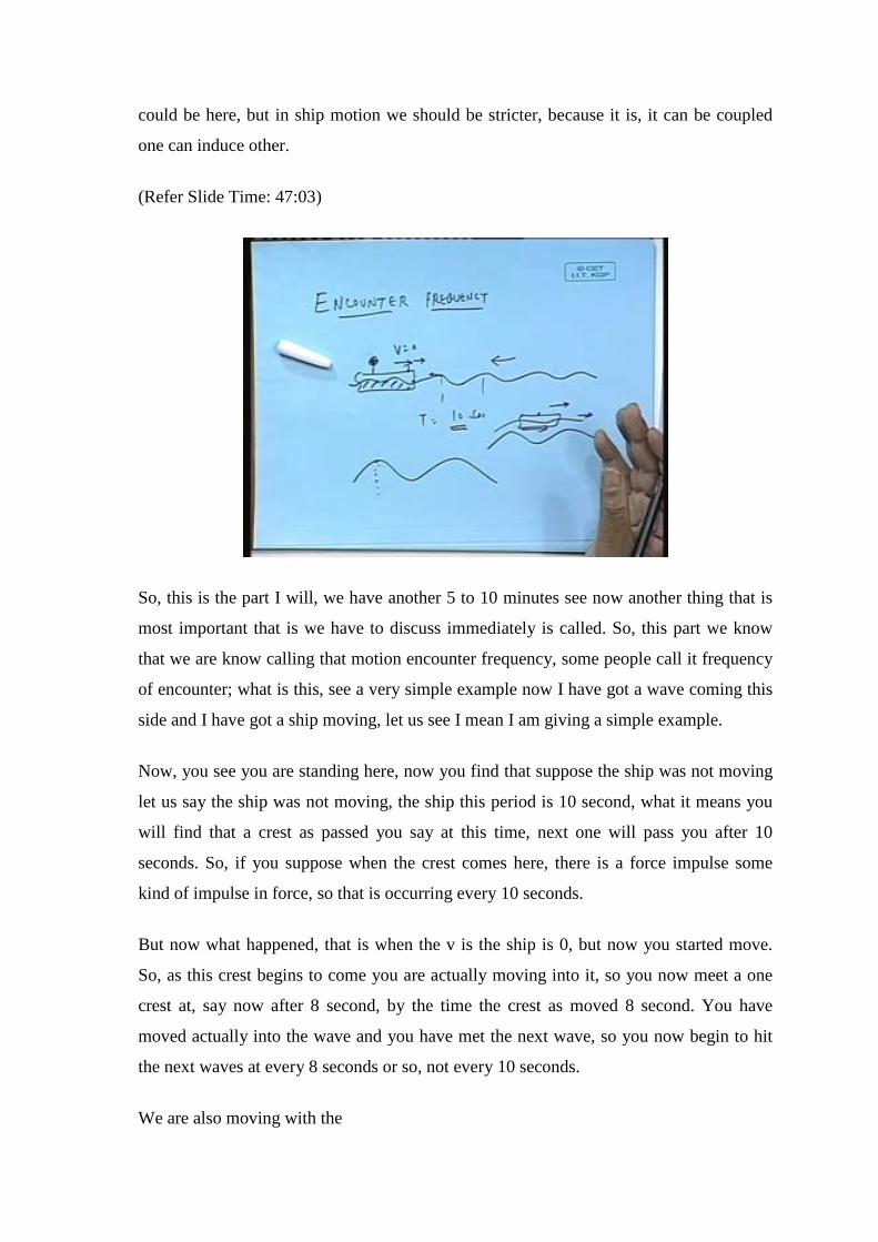
of encounter; what is this, see a very simple example now I have got a wave coming this

side and I have got a ship moving, let us see I mean I am giving a simple example.

Now, you see you are standing here, now you find that suppose the ship was not moving

let us say the ship was not moving, the ship this period is 10 second, what it means you

will find that a crest as passed you say at this time, next one will pass you after 10

seconds. So, if you suppose when the crest comes here, there is a force impulse some

kind of impulse in force, so that is occurring every 10 seconds.

But now what happened, that is when the v is the ship is 0, but now you started move.

So, as this crest begins to come you are actually moving into it, so you now meet a one

crest at, say now after 8 second, by the time the crest as moved 8 second. You have

moved actually into the wave and you have met the next wave, so you now begin to hit

the next waves at every 8 seconds or so, not every 10 seconds.

We are also moving with the

Yes, if we now, if you are going into the wave, if you are going away from the wave that

is a different thing, but I wanted to tell you is that depending on the relative speed

between the two you end up meeting the waves different; in other words, if you are

standing here, you know you know if you are on the ship you are standing here, you

know this observation point here. To you the wave should not appear to have 10 second,

but some other period, because you are moving into the waves, you are a moving frame

of reference and the wave, the ship, the kind of excitation it experiences would be at that

period, why?

See, this I tell always that what is happening to the ship as the wave passes by every

point there is a pressure; each pressure you add up you get a force. We have say, told

earlier that all the pressures every quantity is having same period at 10 second, because

you know everything is sin omega T, that make sense because see when the wave is

passing by this point there is a pressure, when same pressure will be repeating after 10

seconds. So, the net force also will be periodic with the same period, because you know

see here there is a pressure points, now the same thing repeats exactly after 10 seconds,

so it will, it is repetitive after only that period.

But in this case now it is repeating after 8 seconds or whatever seconds, because you are

now going into it therefore, the ship gives a kind of if I think a ship getting a push is

earlier it was getting a push at every 10 seconds, but now it is going to get a push at

every 8 seconds.

This is what we call encounter frequency, you take another case of opposite case the

waves are moving and you are also moving. In fact, if you know I have just draw this

outside, say if may happen that the wave speed and your speed is exactly same. If you

stand here you will you will not feel that you are moving there is any wave, you will

think that you are stationary because, you look at outside and you see that the same crest

is right here I am moving along with that.

So, no impulsive force comes on you, so you do not feel kind of excitation, so there if

frequency of encounter becomes so called the period is 0. So, this is called encounter

frequency which is very critical, because the period at which the ship experiences

excitation is not the period of the absolute wave, but because the the, but something else

as observed by moving ship. So, we have to first come with a formula for what is that

that period.

If the aim of the ship are moving are about the same speed then that he know encounter

the curve.

Exactly there is now you know that this is

Infect


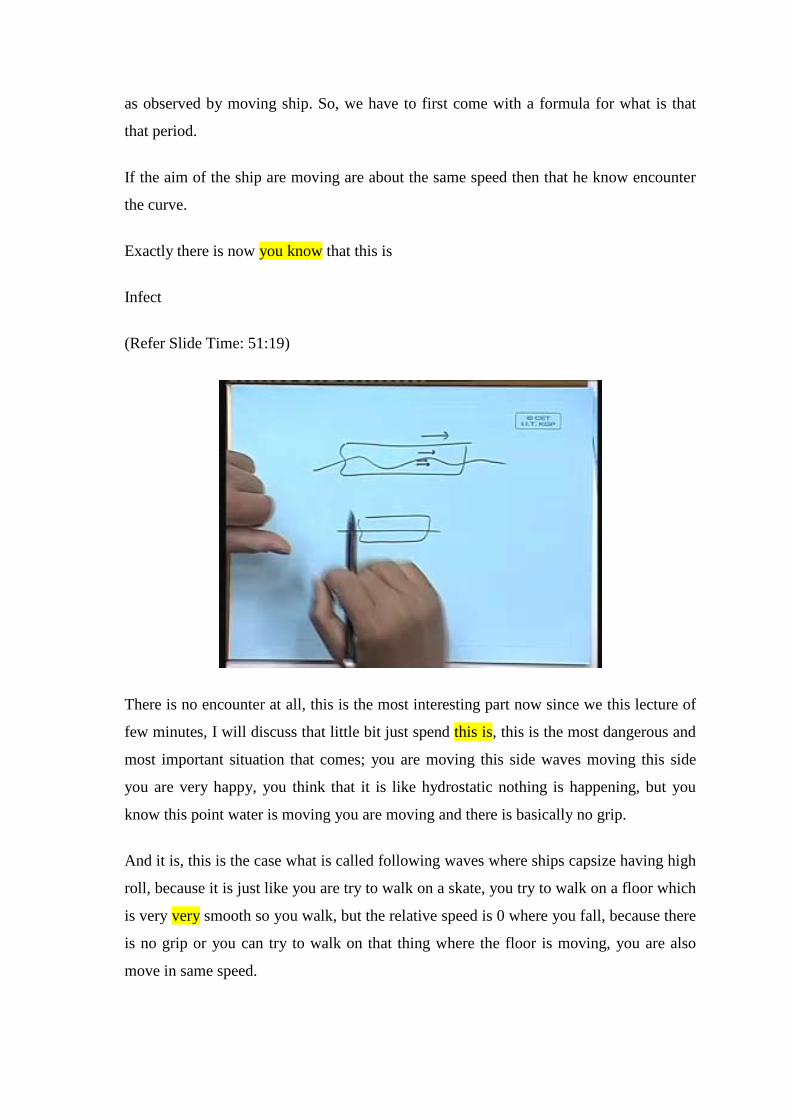
There is no encounter at all, this is the most interesting part now since we this lecture of

few minutes, I will discuss that little bit just spend this is, this is the most dangerous and

most important situation that comes; you are moving this side waves moving this side

you are very happy, you think that it is like hydrostatic nothing is happening, but you

know this point water is moving you are moving and there is basically no grip.

And it is, this is the case what is called following waves where ships capsize having high

roll, because it is just like you are try to walk on a skate, you try to walk on a floor which

is very very smooth so you walk, but the relative speed is 0 where you fall, because there

is no grip or you can try to walk on that thing where the floor is moving, you are also

move in same speed.

You see or it is experience of trying to drive on a ice rink we in Canada use to do that no

grip, just like that it is if you relax saying that there is no waves, you are going to capsize

it is the most dangerous situation of following waves parametric resonance. This we I

will discuss that later on, this is a normally, this is what is called up resonance a large

oscillation of roll motion and there have been accidents for that. Anyhow today, at this

lecture I will end here, we will do in the next lecture, we will pick up from this point

thank you.

Heard about this for thinking us

This we did not here it.

Preview of Next Lecture

Lecture No. # 26

Ship Motion in Regular Waves-II


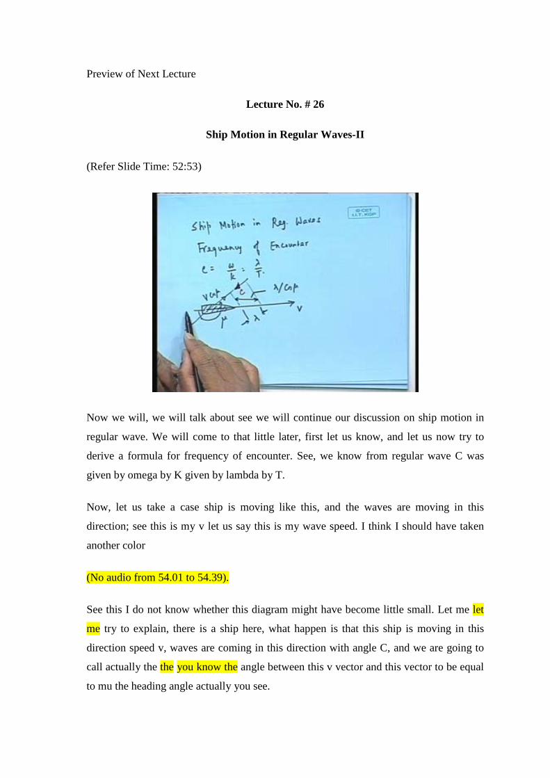
Now we will, we will talk about see we will continue our discussion on ship motion in

regular wave. We will come to that little later, first let us know, and let us now try to

derive a formula for frequency of encounter. See, we know from regular wave C was

given by omega by K given by lambda by T.

Now, let us take a case ship is moving like this, and the waves are moving in this

direction; see this is my v let us say this is my wave speed. I think I should have taken

another color

(No audio from 54.01 to 54.39).

See this I do not know whether this diagram might have become little small. Let me let

me try to explain, there is a ship here, what happen is that this ship is moving in this

direction speed v, waves are coming in this direction with angle C, and we are going to

call actually the the you know the angle between this v vector and this vector to be equal

to mu the heading angle actually you see.


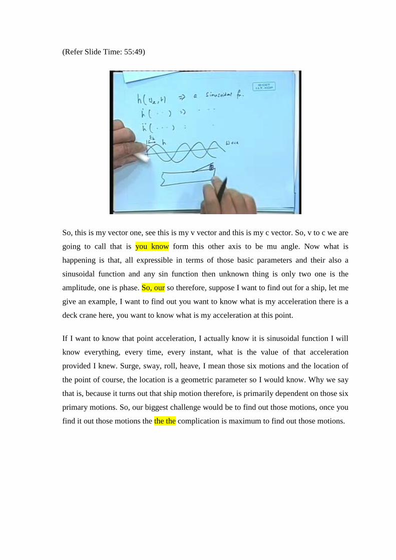
So, this is my vector one, see this is my v vector and this is my c vector. So, v to c we are

going to call that is you know form this other axis to be mu angle. Now what is

happening is that, all expressible in terms of those basic parameters and their also a

sinusoidal function and any sin function then unknown thing is only two one is the

amplitude, one is phase. So, our so therefore, suppose I want to find out for a ship, let me

give an example, I want to find out you want to know what is my acceleration there is a

deck crane here, you want to know what is my acceleration at this point.

If I want to know that point acceleration, I actually know it is sinusoidal function I will

know everything, every time, every instant, what is the value of that acceleration

provided I knew. Surge, sway, roll, heave, I mean those six motions and the location of

the point of course, the location is a geometric parameter so I would know. Why we say

that is, because it turns out that ship motion therefore, is primarily dependent on those six

primary motions. So, our biggest challenge would be to find out those motions, once you

find it out those motions the the the complication is maximum to find out those motions.


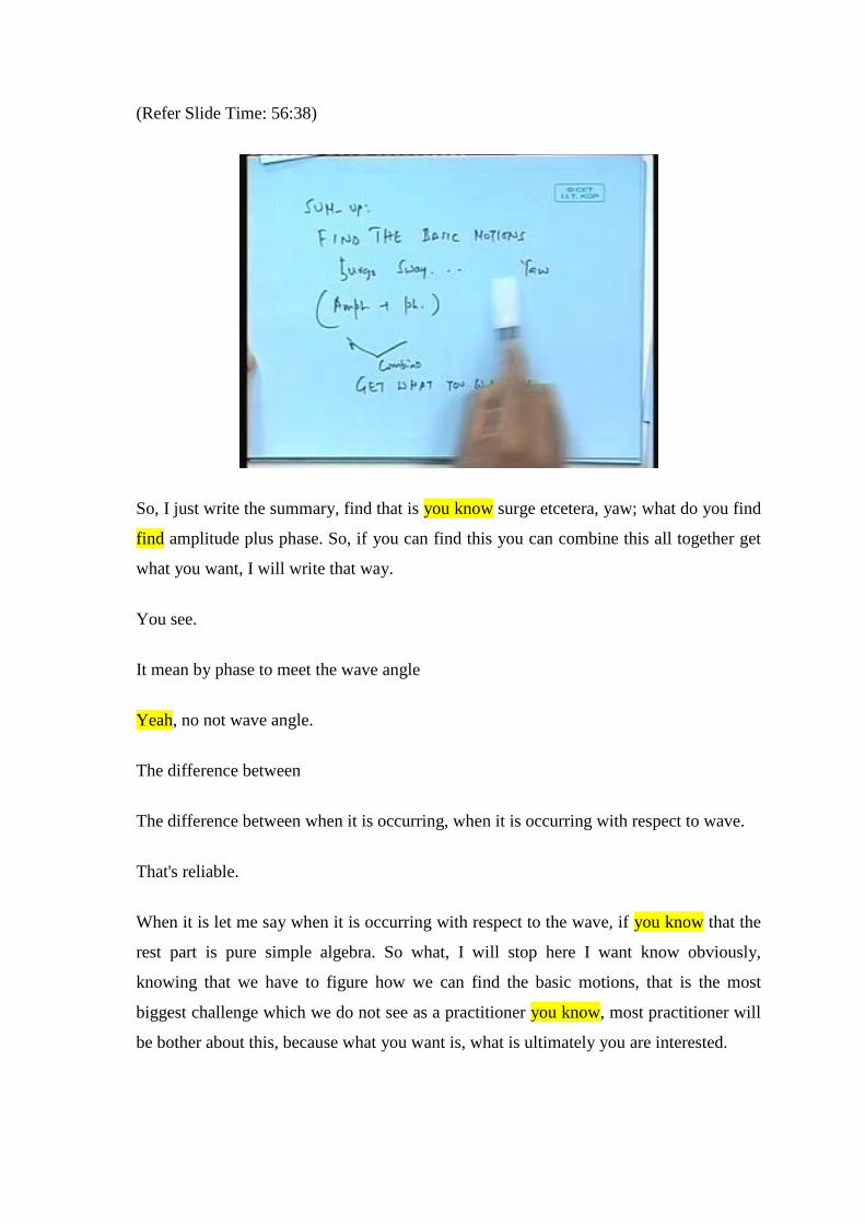
So, I just write the summary, find that is you know surge etcetera, yaw; what do you find

find amplitude plus phase. So, if you can find this you can combine this all together get

what you want, I will write that way.

You see.

It mean by phase to meet the wave angle

Yeah, no not wave angle.

The difference between

The difference between when it is occurring, when it is occurring with respect to wave.

That's reliable.

When it is let me say when it is occurring with respect to the wave, if you know that the

rest part is pure simple algebra. So what, I will stop here I want know obviously,

knowing that we have to figure how we can find the basic motions, that is the most

biggest challenge which we do not see as a practitioner you know, most practitioner will

be bother about this, because what you want is, what is ultimately you are interested.

But to get from here to there is actually algebra simple algebra to get to this point is the

most difficult point you know, but here to here is absolutely simple algebra it is just

question of two more pages of, just doing one it is like if you have to add 10 tables in a

figure it is just t d s, but nothing brainy.

lec25

Documents

Transcript of lec25