lec04_Logic Synthesis.pdf
49
1 Introduction to Electronic Design Automation Jie-Hong Roland Jiang 江介宏 Department of Electrical Engineering National Taiwan University Spring 2014 2 Logic Synthesis High-level synthesis Logic synthesis Physical design Part of the slides are by courtesy of Prof. Andreas Kuehlmann
-
Upload
peter26194 -
Category
Documents
-
view
232 -
download
1
Transcript of lec04_Logic Synthesis.pdf
1
Introduction to Electronic Design Automation
Jie-Hong Roland Jiang江介宏
Department of Electrical EngineeringNational Taiwan University
Spring 2014
2
Logic Synthesis
High-level synthesis
Logic synthesis
Physical design
Part of the slides are by courtesy of Prof. Andreas Kuehlmann
3
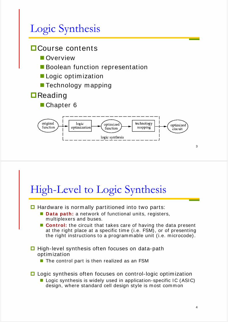
Logic Synthesis
Course contentsOverviewBoolean function representation Logic optimization Technology mapping
ReadingChapter 6
4
High-Level to Logic Synthesis Hardware is normally partitioned into two parts:
Data path: a network of functional units, registers, multiplexers and buses.
Control: the circuit that takes care of having the data present at the right place at a specific time (i.e. FSM), or of presenting the right instructions to a programmable unit (i.e. microcode).
High-level synthesis often focuses on data-path optimization The control part is then realized as an FSM
Logic synthesis often focuses on control-logic optimization Logic synthesis is widely used in application-specific IC (ASIC)
design, where standard cell design style is most common

5
Standard-Cell Based Design
6
Transformation of Logic Synthesis
D
x y
Given: Functional description of finite-state machine F(Q,X,Y,,) where:
Q: Set of internal statesX: Input alphabetY: Output alphabet: X x Q Q (next state function): X x Q Y (output function)
Target: Circuit C(G, W) where:G: set of circuit components g {gates, FFs, etc.}W: set of wires connecting G
7
Boolean Function Representation
Logic synthesis translates Boolean functions into circuits
We need representations of Boolean functions for two reasons: to represent and manipulate the actual circuit
that we are implementing to facilitate Boolean reasoning
8
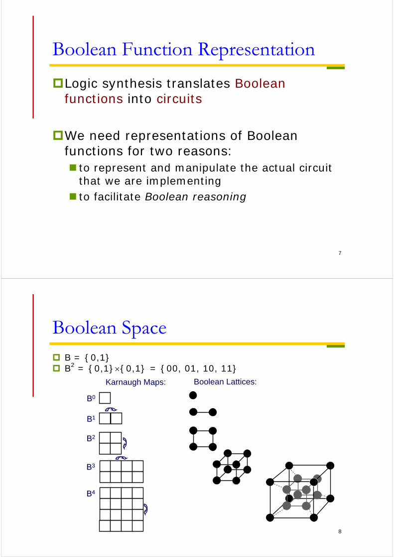
Boolean Space B = {0,1} B2 = {0,1}{0,1} = {00, 01, 10, 11}
Karnaugh Maps: Boolean Lattices:
BB00
BB11
BB22
BB33
BB44
9
Boolean Function A Boolean function f over input variables: x1, x2, …, xm, is a
mapping f: Bm Y, where B = {0,1} and Y = {0,1,d} E.g. The output value of f(x1, x2, x3), say, partitions Bm into three sets:
on-set (f =1) E.g. {010, 011, 110, 111} (characteristic function f1 = x2 )
off-set (f = 0) E.g. {100, 101} (characteristic function f0 = x1 x2 )
don’t-care set (f = d) E.g. {000, 001} (characteristic function fd = x1 x2 )
f is an incompletely specified function if the don’t-care set is nonempty. Otherwise, f is a completely specified function Unless otherwise said, a Boolean function is meant to be completely
specified
10
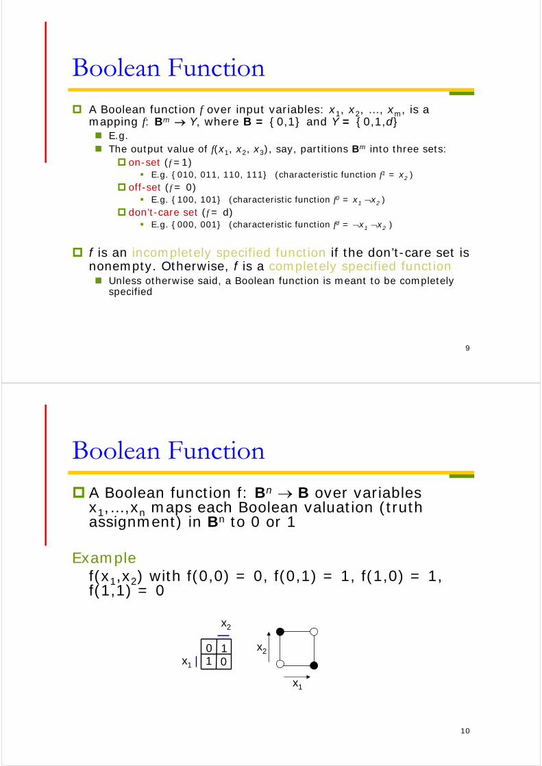
Boolean Function
A Boolean function f: Bn B over variables x1,…,xn maps each Boolean valuation (truth assignment) in Bn to 0 or 1
Examplef(x1,x2) with f(0,0) = 0, f(0,1) = 1, f(1,0) = 1, f(1,1) = 0
001
1x2
x1
x1
x2
11
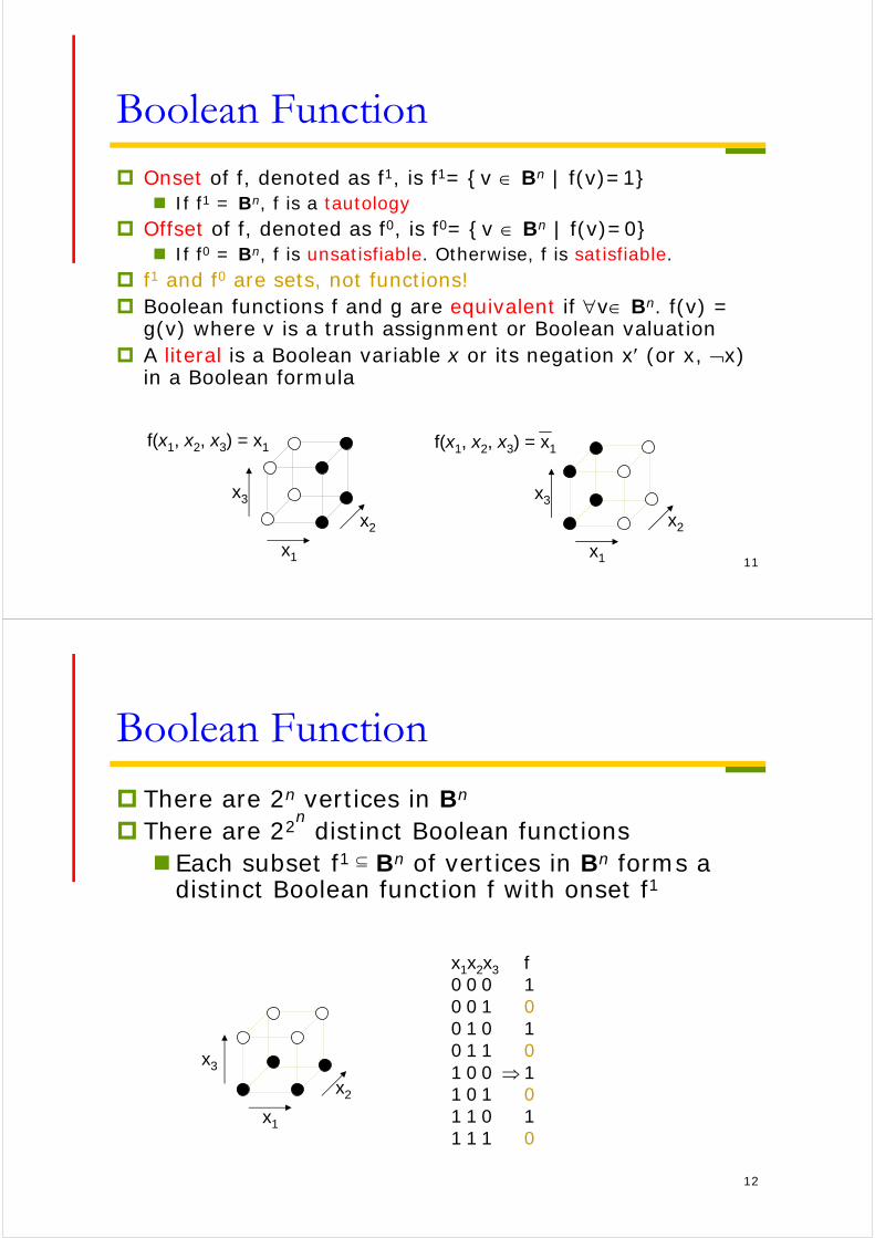
Boolean Function Onset of f, denoted as f1, is f1= {v Bn | f(v)=1}
If f1 = Bn, f is a tautology Offset of f, denoted as f0, is f0= {v Bn | f(v)=0}
If f0 = Bn, f is unsatisfiable. Otherwise, f is satisfiable. f1 and f0 are sets, not functions! Boolean functions f and g are equivalent if v Bn. f(v) =
g(v) where v is a truth assignment or Boolean valuation A literal is a Boolean variable x or its negation x (or x, x)
in a Boolean formula
x3
x1
x2
x1
x2
x3
f(x1, x2, x3) = x1 f(x1, x2, x3) = x1
12
Boolean Function
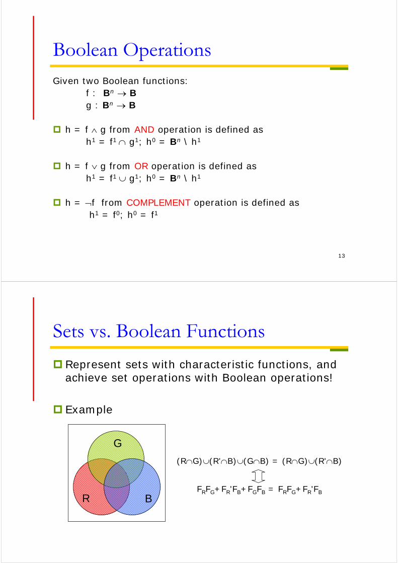
There are 2n vertices in Bn
There are 22n
distinct Boolean functions Each subset f1 Bn of vertices in Bn forms a
distinct Boolean function f with onset f1
x1x2x3 f0 0 0 10 0 1 00 1 0 10 1 1 01 0 0 11 0 1 01 1 0 11 1 1 0
x1
x2
x3
13
Boolean OperationsGiven two Boolean functions:
f : Bn Bg : Bn B
h = f g from AND operation is defined ash1 = f1 g1; h0 = Bn \ h1
h = f g from OR operation is defined ash1 = f1 g1; h0 = Bn \ h1
h = f from COMPLEMENT operation is defined ash1 = f0; h0 = f1
Sets vs. Boolean Functions
Represent sets with characteristic functions, and achieve set operations with Boolean operations!
Example
(RG)(R'B)(GB) = (RG)(R'B)
FRFG+FR'FB+FGFB = FRFG+FR'FBR
G
B

15
Cofactor and QuantificationGiven a Boolean function:
f : Bn B, with the input variable (x1,x2,…,xi,…,xn)
Positive cofactor on variable xih = fxi is defined as h = f(x1,x2,…,1,…,xn)
Negative cofactor on variable xih = fxi is defined as h = f(x1,x2,…,0,…,xn)
Existential quantification over variable xi
h = xi. f is defined as h = f(x1,x2,…,0,…,xn) f(x1,x2,…,1,…,xn)
Universal quantification over variable xi
h = xi. f is defined as h = f(x1,x2,…,0,…,xn) f(x1,x2,…,1,…,xn)
Boolean difference over variable xih = f/xi is defined as h = f(x1,x2,…,0,…,xn) f(x1,x2,…,1,…,xn)
16
Boolean Function Representation Some common representations:
Truth table Boolean formula
SOP (sum-of-products, or called disjunctive normal form, DNF) POS (product-of-sums, or called conjunctive normal form, CNF)
BDD (binary decision diagram) Boolean network (consists of nodes and wires)
Generic Boolean network Network of nodes with generic functional representations or even
subcircuits Specialized Boolean network
Network of nodes with SOPs (PLAs) And-Inv Graph (AIG)
Why different representations? Different representations have their own strengths and
weaknesses (no single data structure is best for all applications)

17
Boolean Function RepresentationTruth Table Truth table (function table for multi-valued
functions):The truth table of a function f : Bn B is a tabulation of its value at each of the 2n
vertices of Bn.
In other words the truth table lists all mintemsExample: f = abcd + abcd + abcd +
abcd + abcd + abcd + abcd + abcd
The truth table representation is- impractical for large n- canonicalIf two functions are the equal, then their canonical representations are isomorphic.
abcd f0 0000 01 0001 12 0010 03 0011 14 0100 05 0101 16 0110 07 0111 0
abcd f8 1000 09 1001 110 1010 011 1011 112 1100 013 1101 114 1110 115 1111 1
18
Boolean Function RepresentationBoolean Formula
A Boolean formula is defined inductively as an expression with the following formation rules (syntax):
formula ::= ‘(‘ formula ‘)’
| Boolean constant (true or false)
| <Boolean variable>
| formula “+” formula (OR operator)
| formula “” formula (AND operator)
| formula (complement)
Example
f = (x1 x2) + (x3) + ((x4 (x1)))
typically “” is omitted and ‘(‘, ‘)’ are omitted when the operator priority is clear, e.g., f = x1 x2 + x3 + x4 x1
19
Boolean Function RepresentationBoolean Formula in SOP
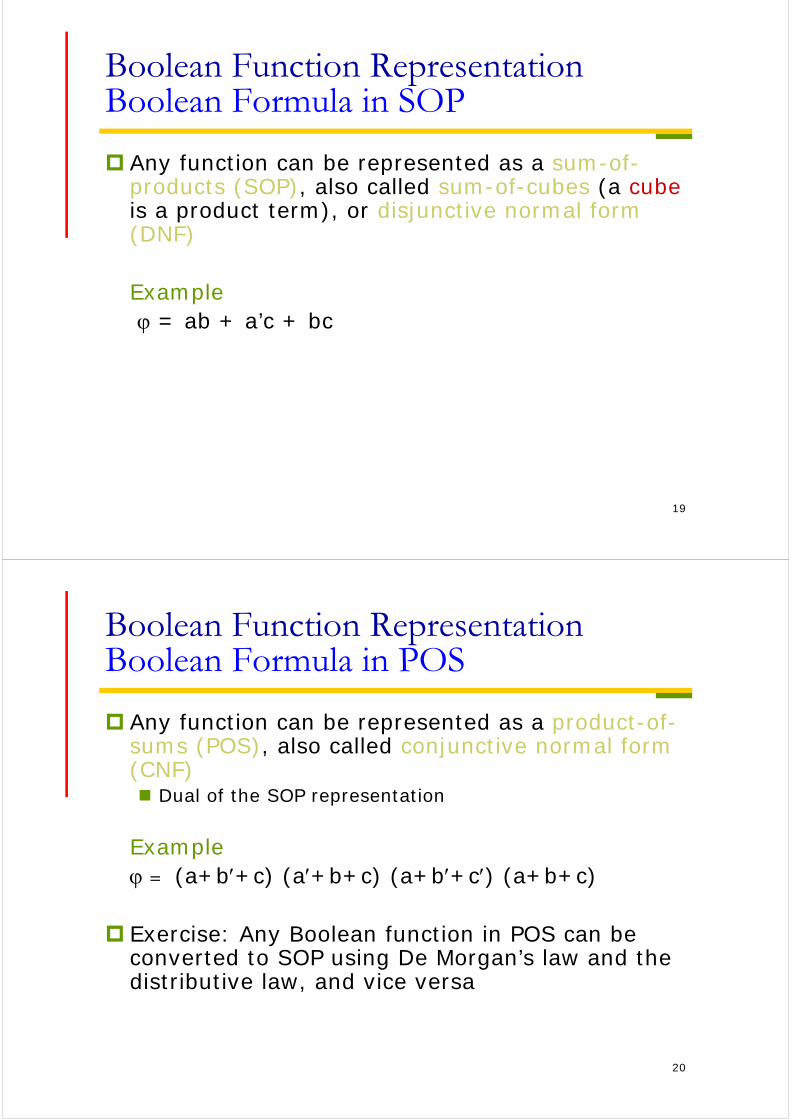
Any function can be represented as a sum-of-products (SOP), also called sum-of-cubes (a cubeis a product term), or disjunctive normal form (DNF)
Example = ab + a’c + bc
20
Boolean Function RepresentationBoolean Formula in POS
Any function can be represented as a product-of-sums (POS), also called conjunctive normal form (CNF) Dual of the SOP representation
Example = (a+b+c) (a+b+c) (a+b+c) (a+b+c)
Exercise: Any Boolean function in POS can be converted to SOP using De Morgan’s law and the distributive law, and vice versa

21
Boolean Function RepresentationBinary Decision Diagram
BDD – a graph representation of Boolean functions A leaf node represents
constant 0 or 1 A non-leaf node
represents a decision node (multiplexer) controlled by some variable
Can make a BDD representation canonicalby imposing the variable ordering and reduction criteria (ROBDD)
f = ab+a’c+a’bd
1
0
c
a
b b
c c
d
0 1
c+bd b
root node
c+d
d
22
Boolean Function RepresentationBinary Decision Diagram
Any Boolean function f can be written in term of Shannon expansion
f = v fv + v fv Positive cofactor: fxi = f(x1,…,xi=1,…, xn) Negative cofactor: fxi = f(x1,…,xi=0,…, xn)
BDD is a compressed Shannon cofactor tree: The two children of a node with function f controlled by
variable v represent two sub-functions fv and fv
v0 1
f
fv fv

23
Boolean Function RepresentationBinary Decision Diagram
Reduced and ordered BDD (ROBDD) is a canonicalBoolean function representation Ordered:
cofactor variables are in the same order along all pathsxi1
< xi2< xi3
< … < xin
Reduced:any node with two identical children is removedtwo nodes with isomorphic BDD’s are merged
These two rules make any node in an ROBDD represent a distinct logic function
a
c c
b
0 1
ordered(a<c<b)
a
b c
c
0 1
notordered
b
a
b
0 1
f
b
0 1
f
reduce
24
Boolean Function RepresentationBinary Decision Diagram
For a Boolean function, ROBDD is unique with respect to a given variable ordering Different orderings may result in different ROBDD structures
a
b b
c c
d
0 1
c+bd b
root node
c+dc
d
f = ab+a’c+bc’d a
c
d
b
0 1
c+bd
db
b
10
leaf node
25
Boolean Function RepresentationBoolean Network
A Boolean network is a directed graph C(G,N) where G are the gates and N GG) are the directed edges (nets) connecting the gates.
Some of the vertices are designated:Inputs: I GOutputs: O G I O =
Each gate g is assigned a Boolean function fgwhich computes the output of the gate in terms of its inputs.
26
Boolean Function RepresentationBoolean Network
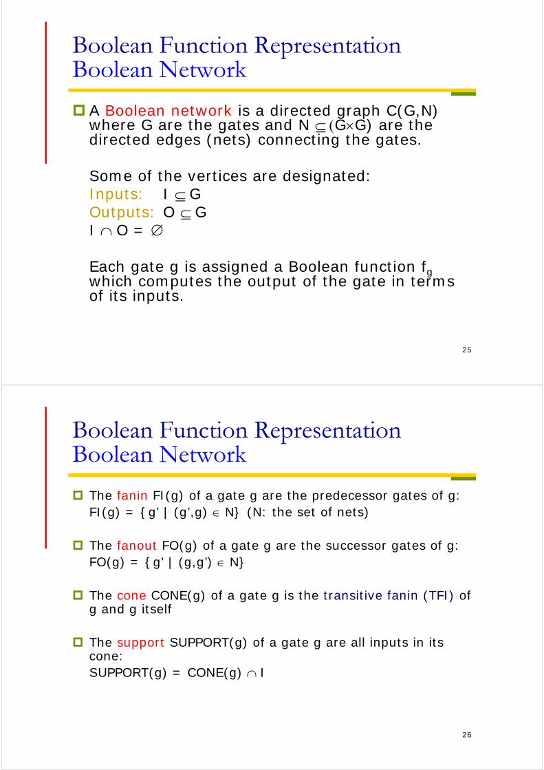
The fanin FI(g) of a gate g are the predecessor gates of g:FI(g) = {g’ | (g’,g) N} (N: the set of nets)
The fanout FO(g) of a gate g are the successor gates of g:FO(g) = {g’ | (g,g’) N}
The cone CONE(g) of a gate g is the transitive fanin (TFI) of g and g itself
The support SUPPORT(g) of a gate g are all inputs in its cone:SUPPORT(g) = CONE(g) I

27
Boolean Function RepresentationBoolean Network
Example
I
O
6
FI(6) = {2,4}
FO(6) = {7,9}
CONE(6) = {1,2,4,6}
SUPPORT(6) = {1,2}
Every node may have its own function
1
5
3
4
78
9
2
28
Boolean Function RepresentationAnd-Inverter Graph
AND-INVERTER graphs (AIGs)vertices: 2-input AND gates edges: interconnects with (optional) dots representing INVs
Hash table to identify and reuse structurally isomorphic circuits
f
g g
f
29
Boolean Function Representation
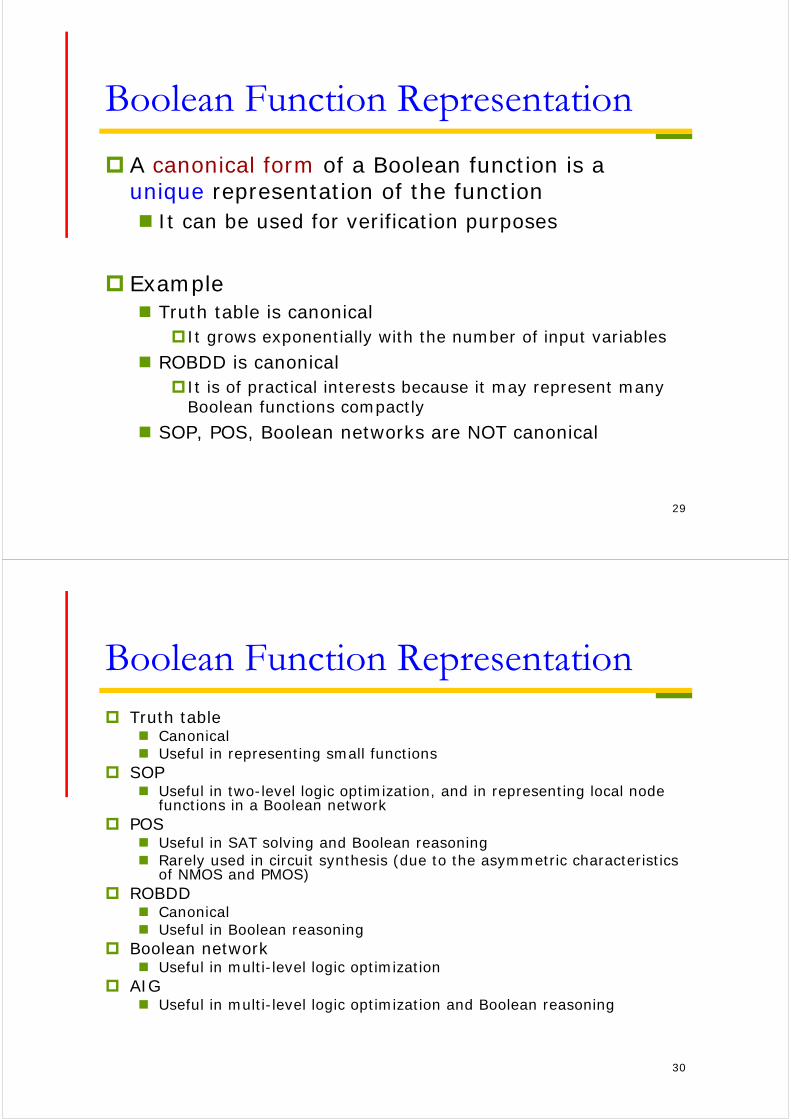
A canonical form of a Boolean function is a unique representation of the function It can be used for verification purposes
Example Truth table is canonical
It grows exponentially with the number of input variables
ROBDD is canonicalIt is of practical interests because it may represent many
Boolean functions compactly
SOP, POS, Boolean networks are NOT canonical
30
Boolean Function Representation Truth table
Canonical Useful in representing small functions
SOP Useful in two-level logic optimization, and in representing local node
functions in a Boolean network POS
Useful in SAT solving and Boolean reasoning Rarely used in circuit synthesis (due to the asymmetric characteristics
of NMOS and PMOS) ROBDD
Canonical Useful in Boolean reasoning
Boolean network Useful in multi-level logic optimization
AIG Useful in multi-level logic optimization and Boolean reasoning

31
Logic Optimization
Boolean functions
two-level optimization
multi-level optimization
technology mapping
circuits
two-level netlists
multi-level netlists
minimized two-level netlists
minimized multi-level netlists
32
Two-Level Logic Minimization
Any Boolean function can be realized using PLA in two levels: AND-OR (sum of products), NAND-NAND, etc. Direct implementation of two-level logic using PLAs
(programmable logic arrays) is not as popular as in the nMOS days
Classic problem solved by the Quine-McCluskeyalgorithm Popular cost function: #cubes and #literals in an SOP
expression#cubes – #rows in a PLA#literals – #transistors in a PLA
The goal is to find a minimal irredundant prime cover

33
Two-Level Logic Minimization
Exact algorithm Quine-McCluskey’s procedure
Heuristic algorithm Espresso
34
Two-Level Logic MinimizationMinterms and Cubes
A minterm is a product of every input variable or its negation A minterm corresponds to a single point in Bn
A cube is a product of literals The fewer the number of literals is in the product,
the bigger the space is covered by the cube
35
Two-Level Logic MinimizationImplicant and Cover
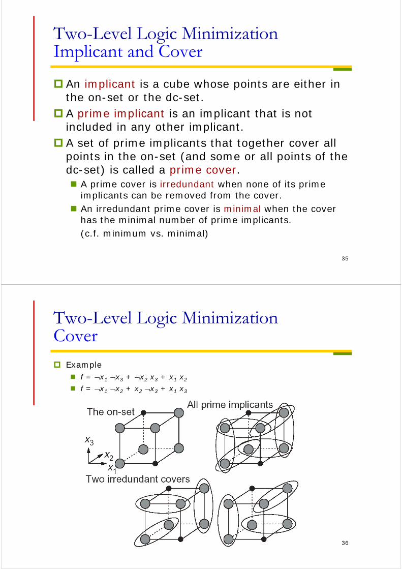
An implicant is a cube whose points are either in the on-set or the dc-set.
A prime implicant is an implicant that is not included in any other implicant.
A set of prime implicants that together cover all points in the on-set (and some or all points of the dc-set) is called a prime cover. A prime cover is irredundant when none of its prime
implicants can be removed from the cover. An irredundant prime cover is minimal when the cover
has the minimal number of prime implicants.(c.f. minimum vs. minimal)
36
Two-Level Logic MinimizationCover
Example f = x1 x3 + x2 x3 + x1 x2
f = x1 x2 + x2 x3 + x1 x3

37
Two-Level Logic MinimizationCover
Example
local minimal global minimal
38
Two-Level Logic MinimizationQuine-McCluskey Procedure
Given G and D (covers for = (f,d,r) and d, respectively), find a minimum cover G* of primes where: f G* f+d (G* is a prime cover of ) f is the onset, d don’t-care set, and r offset
Q-M Procedure:1.Generate all primes of , {Pj} (i.e. primes of (f+d) =
G+D)2.Generate all minterms {mi} of f = GD3.Build Boolean matrix B where
Bij = 1 if mi Pj
= 0 otherwise4.Solve the minimum column covering problem for B
(unate covering problem)

39
Two-Level Logic MinimizationQuine-McCluskey ProcedureGenerating Primes
Tabular method(based on consensus operation):
Start with all minterm canonical form of F
Group pairs of adjacent minterms into cubes
Repeat merging cubes until no more merging possible; mark ()+ remove all covered cubes.
Result: set of primes of f.
Example
F = x’ y’ + w x y + x’ y z’ + w y’ z
w’ x’ y’ z’
w’ x’ y’ z w’ x’ y z’ w x’ y’ z’
w x’ y’ z w x’ y z’
w x y z’ w x y’ z w x y z
w’ x’ y’ w’ x’ z’ x’ y’ z’ x’ y’ z x’ y z’ w x’ y’ w x’ z’ w y’ z
w y z’
w x y
w x z
x’ y’
x’ z’
F = x’ y’ + w x y + x’ y z’ + w y’ z
Courtesy: Maciej Ciesielski, UMASS
40
Example
Primes: y + w +xzCovering TableSolution: {1,2} y + w is a minimum prime cover (also w +xz)
dd
ddd
dd
dd
00
1
11
01
Two-Level Logic MinimizationQuine-McCluskey Procedure
F x y z w xy zw x y zw xyzw
D yz xyw x y zw x y w xy z w
xy xy xy xy
zw
zw
zw
zw
xz
Karnaugh map
010
011
110
101
y w xz
xyz w
x y z w
x yz w
xyzw
(cover of )
(cover of d)
w
y
41
Two-Level Logic MinimizationQuine-McCluskey Procedure
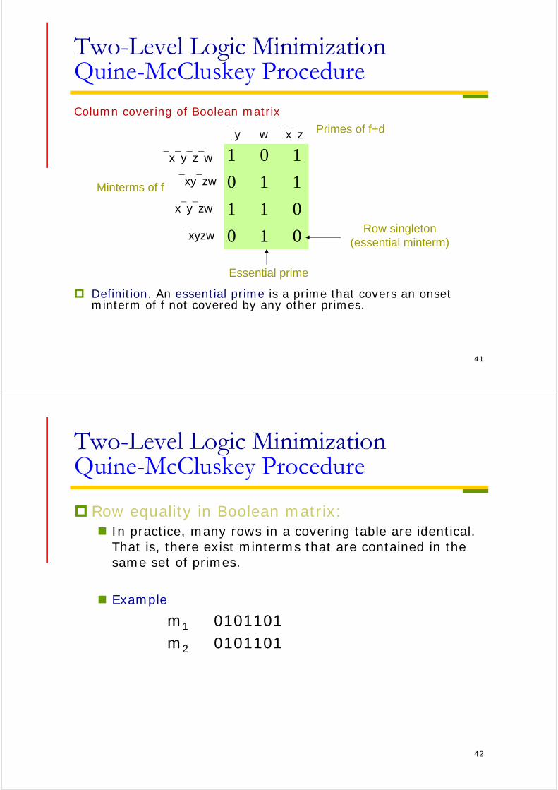
Column covering of Boolean matrix
Definition. An essential prime is a prime that covers an onset minterm of f not covered by any other primes.
010
011
110
101y w xz
xyzw
xyzw
xyzw
xyzw
Primes of f+d
Minterms of f
Essential prime
Row singleton(essential minterm)
42
Two-Level Logic MinimizationQuine-McCluskey Procedure
Row equality in Boolean matrix: In practice, many rows in a covering table are identical.
That is, there exist minterms that are contained in the same set of primes.
Example
m1 0101101m2 0101101
43
Two-Level Logic MinimizationQuine-McCluskey Procedure
Row dominance in Boolean matrix: A row i1 whose set of primes is contained in the set of
primes of row i2 is said to dominate i2.
Example
i1 011010i2 011110
i1 dominates i2Can remove row i2 because have to choose a prime to
cover i1, and any such prime also covers i2. So i2 is automatically covered.
44
Two-Level Logic MinimizationQuine-McCluskey Procedure
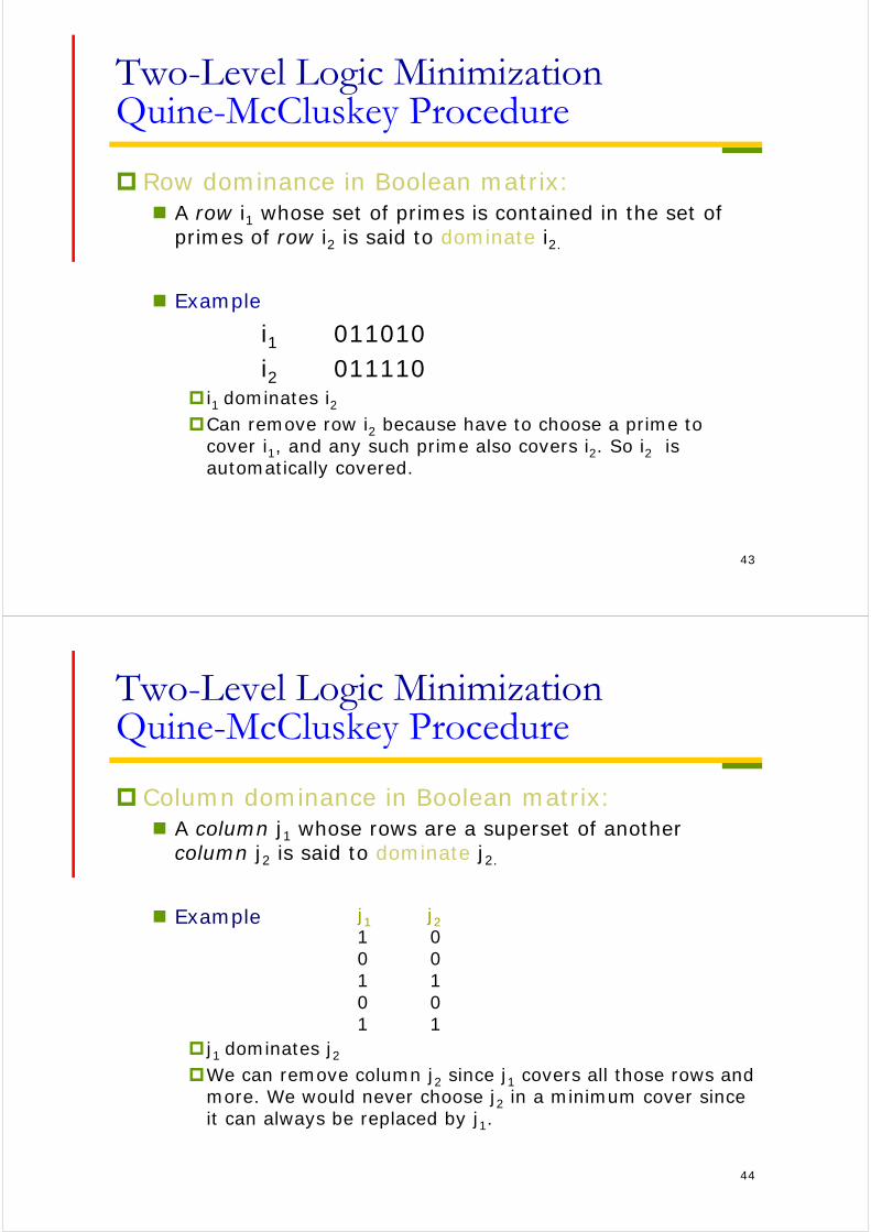
Column dominance in Boolean matrix: A column j1 whose rows are a superset of another
column j2 is said to dominate j2.
Example
j1 dominates j2We can remove column j2 since j1 covers all those rows and
more. We would never choose j2 in a minimum cover since it can always be replaced by j1.
j1 j21 00 01 10 01 1
45
Two-Level Logic MinimizationQuine-McCluskey Procedure
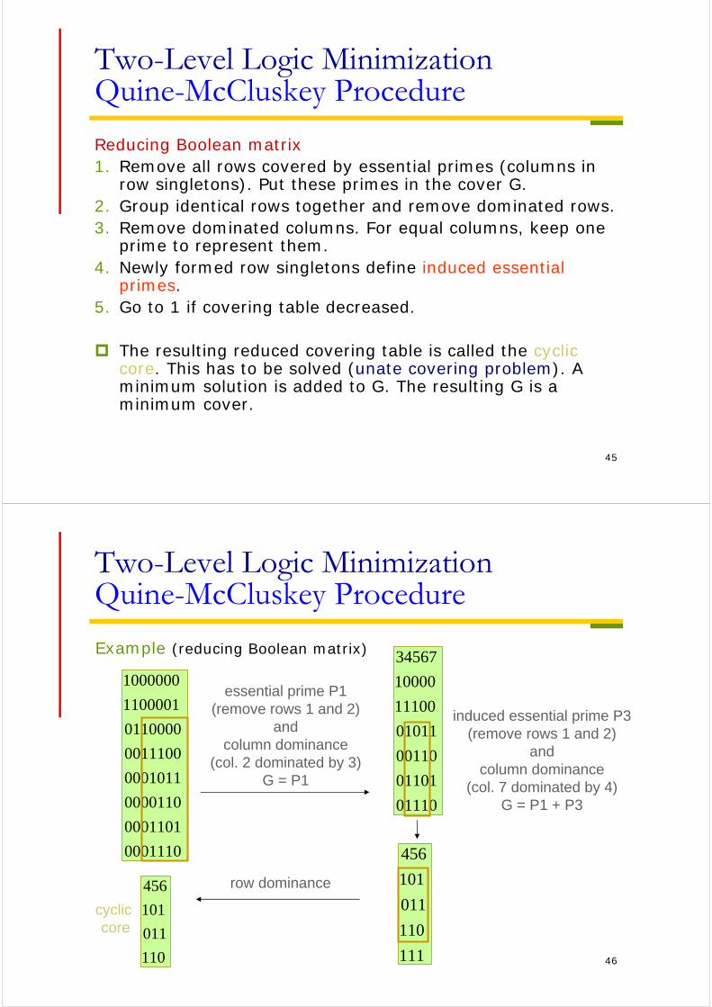
Reducing Boolean matrix 1. Remove all rows covered by essential primes (columns in
row singletons). Put these primes in the cover G.2. Group identical rows together and remove dominated rows.3. Remove dominated columns. For equal columns, keep one
prime to represent them.4. Newly formed row singletons define induced essential
primes.5. Go to 1 if covering table decreased.
The resulting reduced covering table is called the cyclic core. This has to be solved (unate covering problem). A minimum solution is added to G. The resulting G is a minimum cover.
46
Two-Level Logic MinimizationQuine-McCluskey Procedure
Example (reducing Boolean matrix)
0001110
0001101
0000110
0001011
0011100
0110000
1100001
1000000
01110
01101
00110
01011
11100
10000
34567
induced essential prime P3(remove rows 1 and 2)
andcolumn dominance
(col. 7 dominated by 4)G = P1 + P3
111
110
011
101
456
110
011
101
456
essential prime P1 (remove rows 1 and 2)
and column dominance
(col. 2 dominated by 3)G = P1
row dominance
cyclic core
47
Two-Level Logic MinimizationQuine-McCluskey Procedure
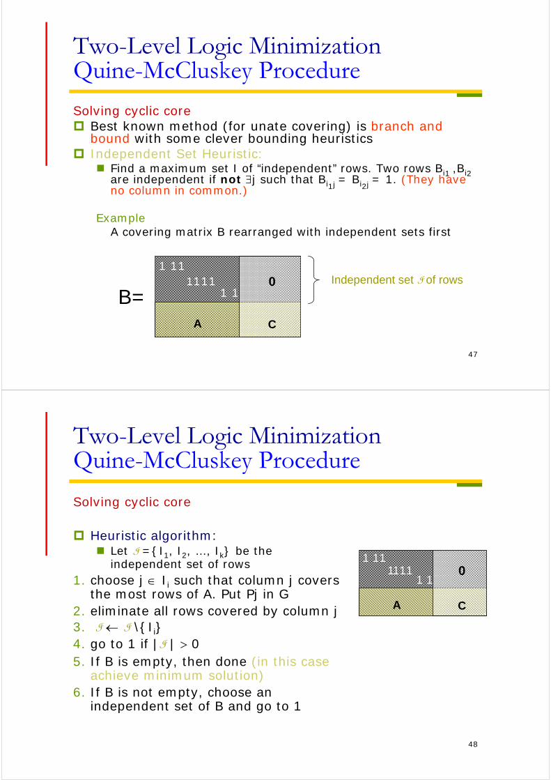
Solving cyclic core Best known method (for unate covering) is branch and
bound with some clever bounding heuristics Independent Set Heuristic:
Find a maximum set I of “independent” rows. Two rows Bi1 ,Bi2 are independent if not j such that Bi1j = Bi2j = 1. (They have no column in common.)
ExampleA covering matrix B rearranged with independent sets first
Independent set I of rows11
111111
0
A
1
C
B=
48
Two-Level Logic MinimizationQuine-McCluskey Procedure
Solving cyclic core
Heuristic algorithm: Let I ={I1, I2, …, Ik} be the
independent set of rows1. choose j Ii such that column j covers
the most rows of A. Put Pj in G2. eliminate all rows covered by column j3. I I \{Ii}4. go to 1 if |I | 05. If B is empty, then done (in this case
achieve minimum solution)6. If B is not empty, choose an
independent set of B and go to 1
111111
110
A
1
C

49
Two-Level Logic MinimizationQuine-McCluskey Procedure
SummaryCalculate all prime implicants (of the union of
the onset and don’t care set) Find the minimal cover of all minterms in the
onset by prime implicantsConstruct the covering matrixSimplify the covering matrix by detecting essential
columns, row and column dominanceWhat is left is the cyclic core of the covering matrix.
The covering problem can then be solved by a branch-and-bound algorithm.
50
Two-Level Logic MinimizationExact vs. Heuristic Algorithms
Quine-McCluskey Method:1.Generate cover of all primes G = p1 + p2 ++p3n/n
2.Make G irredundant (in optimum way) Q-M is exact, i.e., it gives an exact minimum
Heuristic Methods:1.Generate (somehow) a cover of using some of
the primes G = pi1+ pi2
+ + pik
2.Make G irredundant (maybe not optimally)3.Keep best result - try again (i.e. go to 1)

51
Two-Level Logic MinimizationESPRESSO
Heuristic two-level logic minimization
ESPRESSO()
{
(F,D,R) DECODE()
F EXPAND(F,R)
F IRREDUNDANT(F,D)
E ESSENTIAL_PRIMES(F,D)
F F-E; D D E
do{
do{
F REDUCE(F,D)
F EXPAND(F,R)
F IRREDUNDANT(F,D)
}while fewer terms in F
//LASTGASP
G REDUCE_GASP(F,D)
G EXPAND(G,R)
F IRREDUNDANT(F G,D)
}while fewer terms in F
F F E; D D-E
LOWER_OUTPUT(F,D)
//LASTGASP
RAISE_INPUTS
old old
(F,R)
error (F F) or (F F D)
return (F,error)
}
52
Two-Level Logic MinimizationESPRESSO
Local minimum
Local minimum
REDUCE
EXPAND
IRREDANDANT
53
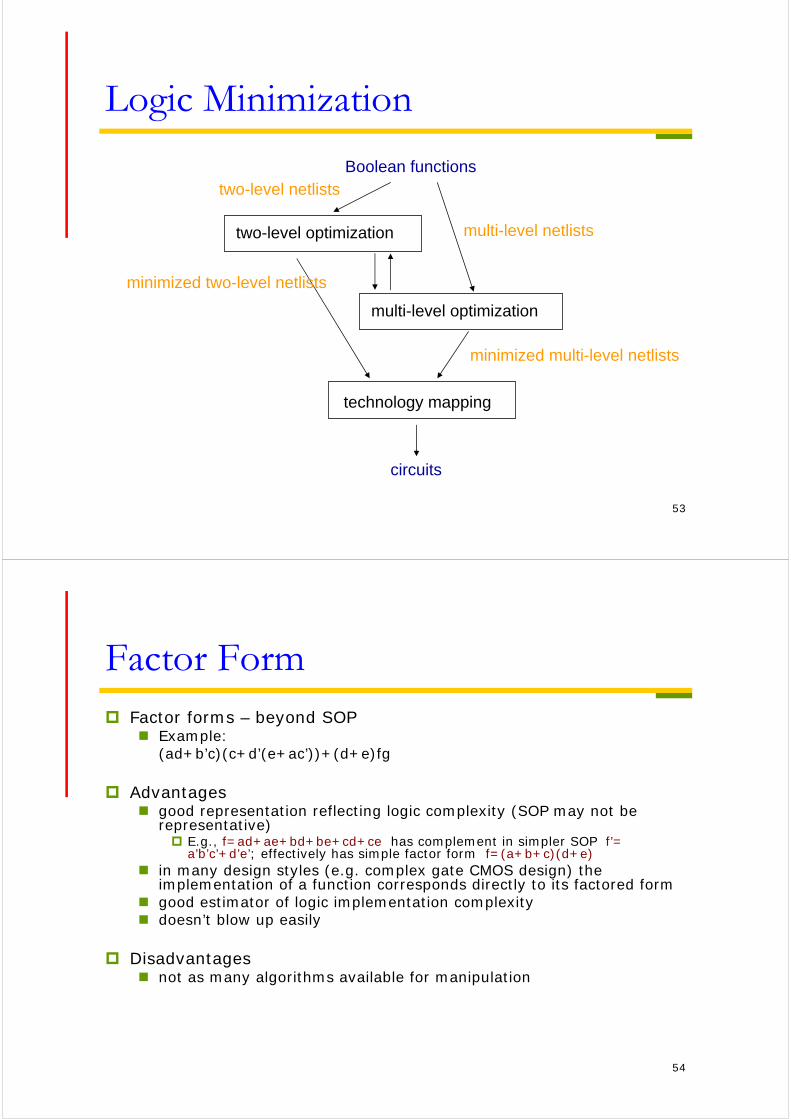
Logic Minimization
Boolean functions
two-level optimization
multi-level optimization
technology mapping
circuits
two-level netlists
multi-level netlists
minimized two-level netlists
minimized multi-level netlists
54
Factor Form Factor forms – beyond SOP
Example: (ad+b’c)(c+d’(e+ac’))+(d+e)fg
Advantages good representation reflecting logic complexity (SOP may not be
representative) E.g., f=ad+ae+bd+be+cd+ce has complement in simpler SOP f’=
a’b’c’+d’e’; effectively has simple factor form f=(a+b+c)(d+e) in many design styles (e.g. complex gate CMOS design) the
implementation of a function corresponds directly to its factored form good estimator of logic implementation complexity doesn’t blow up easily
Disadvantages not as many algorithms available for manipulation

55
Factor From
Factored forms are useful in estimating area and delay in multi-level logic Note: literal count
transistor count area however, area also
depends on wiring, gate size, etc.
therefore very crude measure
d
b
ac
56
Factor From
There are functions whose sizes are exponential in the SOP representation, but polynomial in the factored form Example
Achilles’ heel function
There are n literals in the factored form and (n/2)2n/2 literals in the SOP form.
(x
2i1 x
2i)
i1
in / 2
57
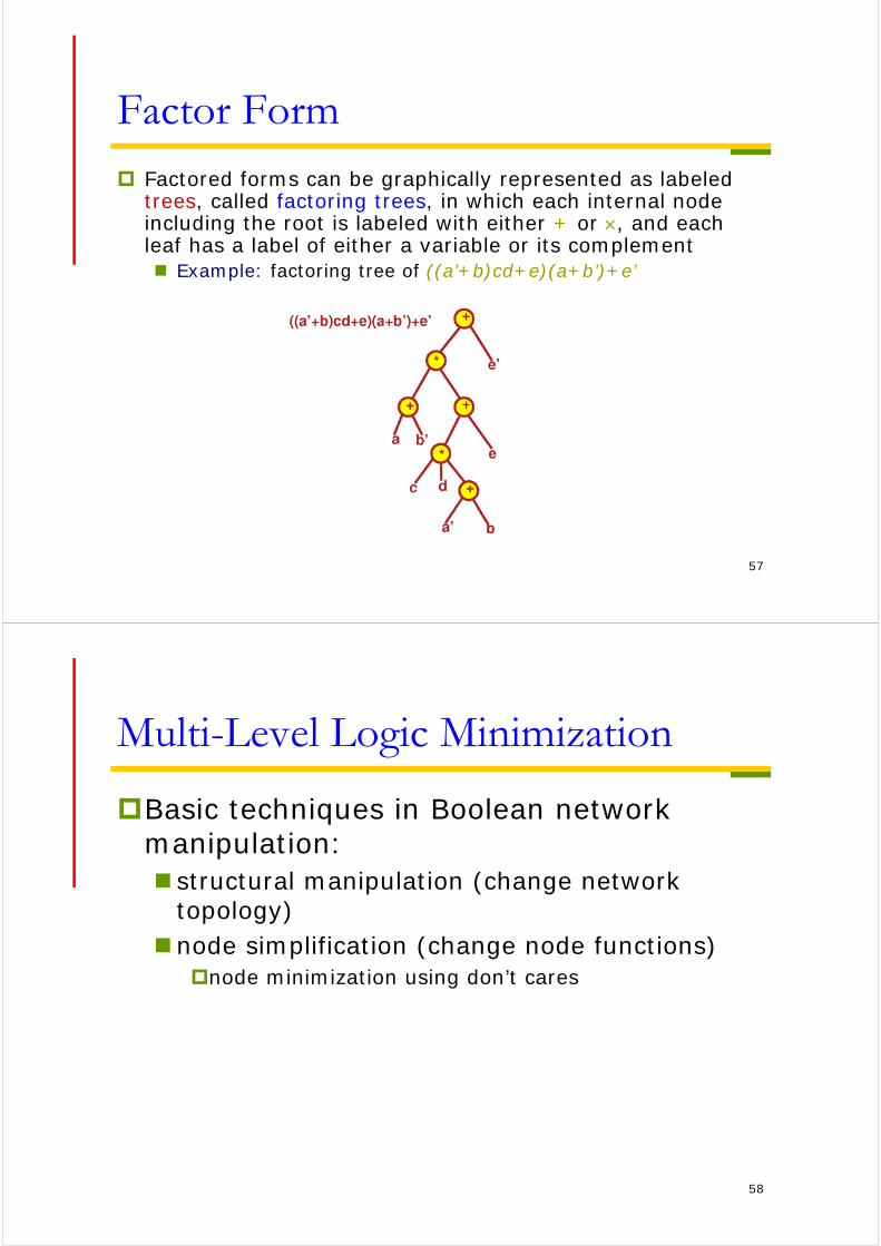
Factor Form Factored forms can be graphically represented as labeled
trees, called factoring trees, in which each internal node including the root is labeled with either + or , and each leaf has a label of either a variable or its complement Example: factoring tree of ((a’+b)cd+e)(a+b’)+e’
58
Multi-Level Logic Minimization
Basic techniques in Boolean network manipulation: structural manipulation (change network
topology) node simplification (change node functions)
node minimization using don’t cares

59
Multi-Level Logic MinimizationStructural ManipulationRestructuring Problem: Given initial network, find best network.
Example:f1 = abcd+abce+ab’cd’+ab’c’d’+a’c+cdf+abc’d’e’+ab’c’df’f2 = bdg+b’dfg+b’d’g+bd’eg
minimizing,f1 = bcd+bce+b’d’+a’c+cdf+abc’d’e’+ab’c’df’f2 = bdg+dfg+b’d’g+d’eg
factoring,f1 = c(b(d+e)+b’(d’+f)+a’)+ac’(bd’e’+b’df’)f2 = g(d(b+f)+d’(b’+e))
decompose,f1 = c(b(d+e)+b’(d’+f)+a’)+ac’x’f2 = gxx = d(b+f)+d’(b’+e)
Two problems: find good common subfunctions effect the division
60
Multi-Level Logic MinimizationStructural Manipulation
Basic operations:1. Decomposition (for a single function)
f = abc+abd+a’c’d’+b’c’d’
f = xy+x’y’ x = ab y = c+d2. Extraction (for multiple functions)
f = (az+bz’)cd+e g = (az+bz’)e’ h = cde
f = xy+e g = xe’ h = ye x = az+bz’ y = cd3. Factoring (series-parallel decomposition)
f = ac+ad+bc+bd+e
f = (a+b)(c+d)+e
61
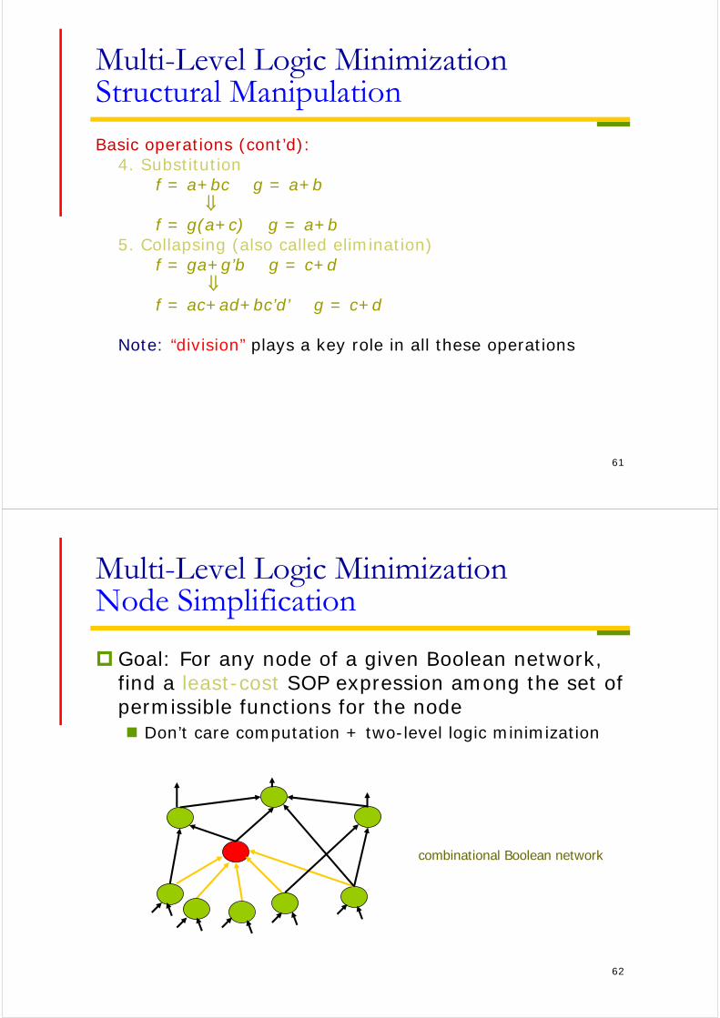
Multi-Level Logic MinimizationStructural Manipulation
Basic operations (cont’d):4. Substitution
f = a+bc g = a+b
f = g(a+c) g = a+b 5. Collapsing (also called elimination)
f = ga+g’b g = c+d
f = ac+ad+bc’d’ g = c+d
Note: “division” plays a key role in all these operations
62
Multi-Level Logic MinimizationNode Simplification
Goal: For any node of a given Boolean network, find a least-cost SOP expression among the set of permissible functions for the node Don’t care computation + two-level logic minimization
combinational Boolean network
63
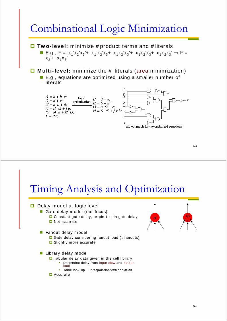
Combinational Logic Minimization Two-level: minimize #product terms and #literals
E.g., F = x1’x2’x3’+ x1’x2’x3+ x1x2’x3’+ x1x2’x3+ x1x2x3’ F = x2’+ x1x3’
Multi-level: minimize the # literals (area minimization) E.g., equations are optimized using a smaller number of
literals
64
Timing Analysis and Optimization Delay model at logic level
Gate delay model (our focus) Constant gate delay, or pin-to-pin gate delay Not accurate
Fanout delay model Gate delay considering fanout load (#fanouts) Slightly more accurate
Library delay model Tabular delay data given in the cell library
Determine delay from input slew and output load
Table look-up + interpolation/extrapolation Accurate
d

65
Timing Analysis and OptimizationGate Delay
The delay of a gate depends on:
1. Output Load Capacitive loading charge
needed to swing the output voltage
Due to interconnect and logic fanout
2. Input Slew Slew = transition time Slower transistor switching
longer delay and longer output slew
e.g. output 1→0
1
0
Vin
Tslew
= ReffCload
CloadCloadReff
An inverter
66
Timing Analysis and OptimizationTiming Library
Timing library contains all relevant information about each standard cell E.g., pin direction, clock, pin
capacitance, etc.
Delay (fastest, slowest, and often typical) and output slew are encoded for each input-to-output path and each pair of transition directions
Values typically represented as 2 dimensional look-up tables (of output load and input slew) Interpolation is used
Output load (nF)
Inpu
t sle
w (
ns)
1.0 2.0 4.0 10.0
0.1 2.1 2.6 3.4 6.1
0.5 2.4 2.9 3.9 7.2
1.0 2.6 3.4 4.0 8.1
2.0 2.8 3.7 4.9 10.3
“delay_table_1”
Path(inputPorts(A), outputPorts(Z), inputTransition(01), outputTransition(10), “delay_table_1”, “output_slew_table_1”
);
A
B
Z
01
10
67
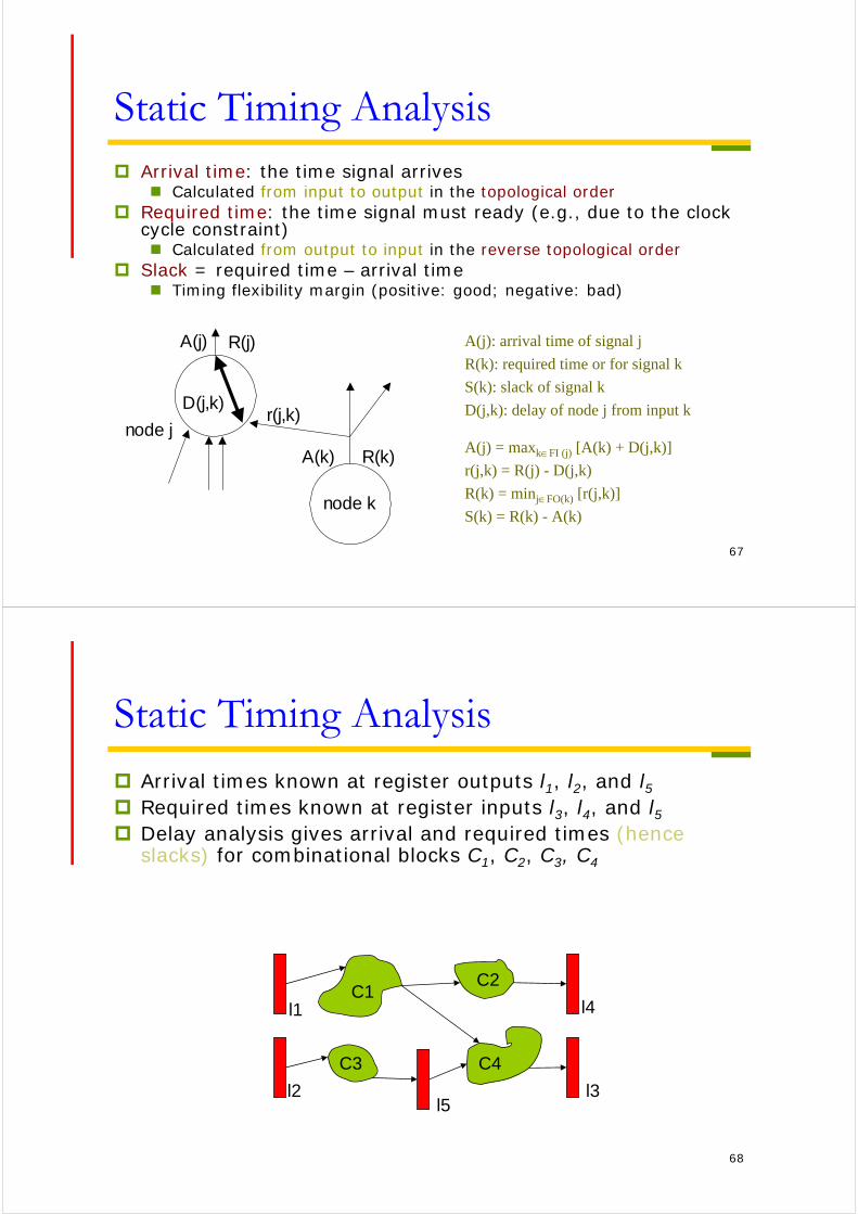
Static Timing Analysis Arrival time: the time signal arrives
Calculated from input to output in the topological order Required time: the time signal must ready (e.g., due to the clock
cycle constraint) Calculated from output to input in the reverse topological order
Slack = required time – arrival time Timing flexibility margin (positive: good; negative: bad)
node k
A(j) R(j)
node j
D(j,k)r(j,k)
A(k) R(k)
A(j): arrival time of signal j
R(k): required time or for signal k
S(k): slack of signal k
D(j,k): delay of node j from input k
A(j) = maxkFI (j) [A(k) + D(j,k)]
r(j,k) = R(j) - D(j,k)
R(k) = minjFO(k) [r(j,k)]
S(k) = R(k) - A(k)
68
Static Timing Analysis Arrival times known at register outputs l1, l2, and l5 Required times known at register inputs l3, l4, and l5 Delay analysis gives arrival and required times (hence
slacks) for combinational blocks C1, C2, C3, C4
C3
C1C2
C4
l1
l2 l3
l4
l5
69
Static Timing Analysis
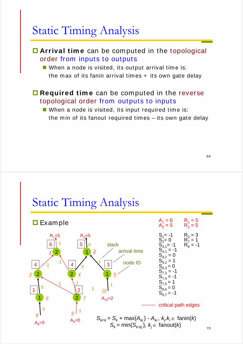
Arrival time can be computed in the topological order from inputs to outputs When a node is visited, its output arrival time is:
the max of its fanin arrival times + its own gate delay
Required time can be computed in the reverse topological order from outputs to inputs When a node is visited, its input required time is:
the min of its fanout required times – its own gate delay
70
Static Timing Analysis
Example
2 1
2 2 1
21
R2=5R1=5
A8=0 A9=0
980
01
0-1
-1-1
-110
-1
-1
5
76
3
1 2
4
1
4
2
34
56
node ID
arrival timeslack
A10=2
101
A1 = 6 R1 = 5A2 = 5 R2 = 5
S1= -1 R3 = 3S2= 0 R7 = 1S3,1= -1 R9 = -1S4,1 = -1S4,2 = 0S5,2 = 1S6,3 = 0S7,3 = -1S7,4 = -1S7,5 = 1S8,6 = 0S9,7 = -1
critical path edges
Ski,k = Sk + max{Akj } - Aki , kj,ki fanin(k)Sk = min{Sk,kj }, kj fanout(k)
71
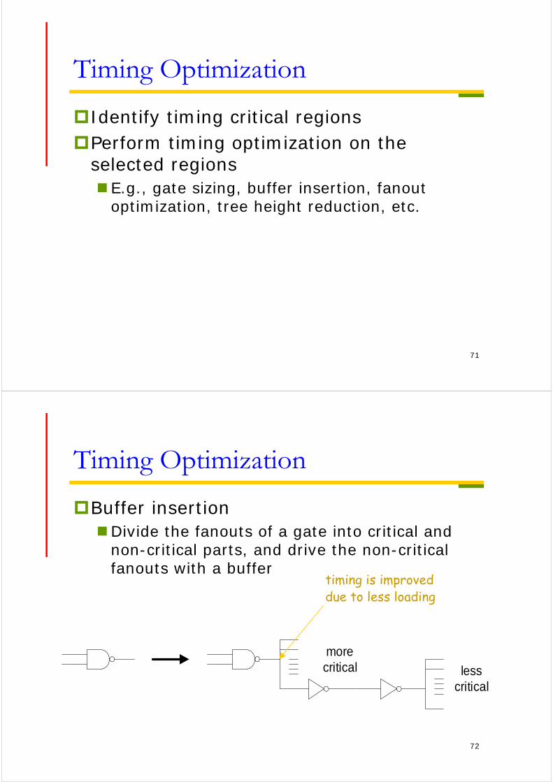
Timing Optimization
Identify timing critical regionsPerform timing optimization on the
selected regions E.g., gate sizing, buffer insertion, fanout
optimization, tree height reduction, etc.
72
Timing Optimization
Buffer insertionDivide the fanouts of a gate into critical and
non-critical parts, and drive the non-critical fanouts with a buffer
morecritical less
critical
timing is improveddue to less loading
73
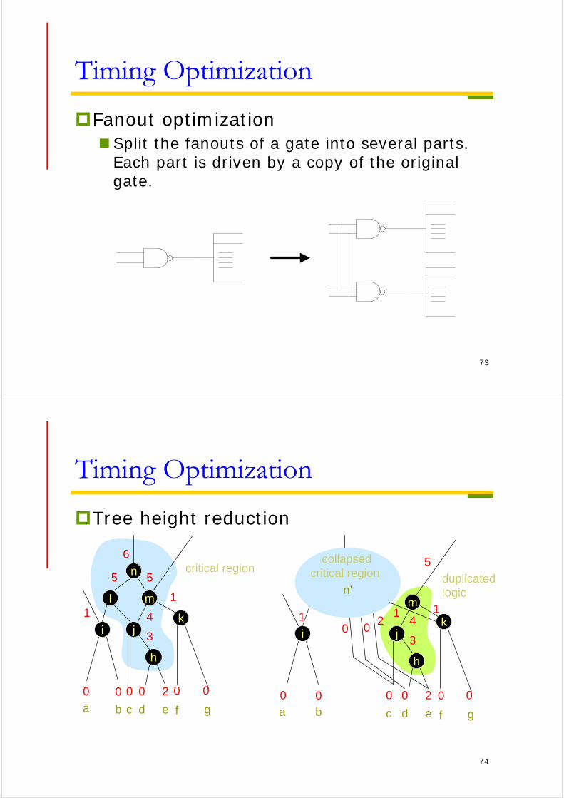
Timing Optimization
Fanout optimizationSplit the fanouts of a gate into several parts.
Each part is driven by a copy of the original gate.
74
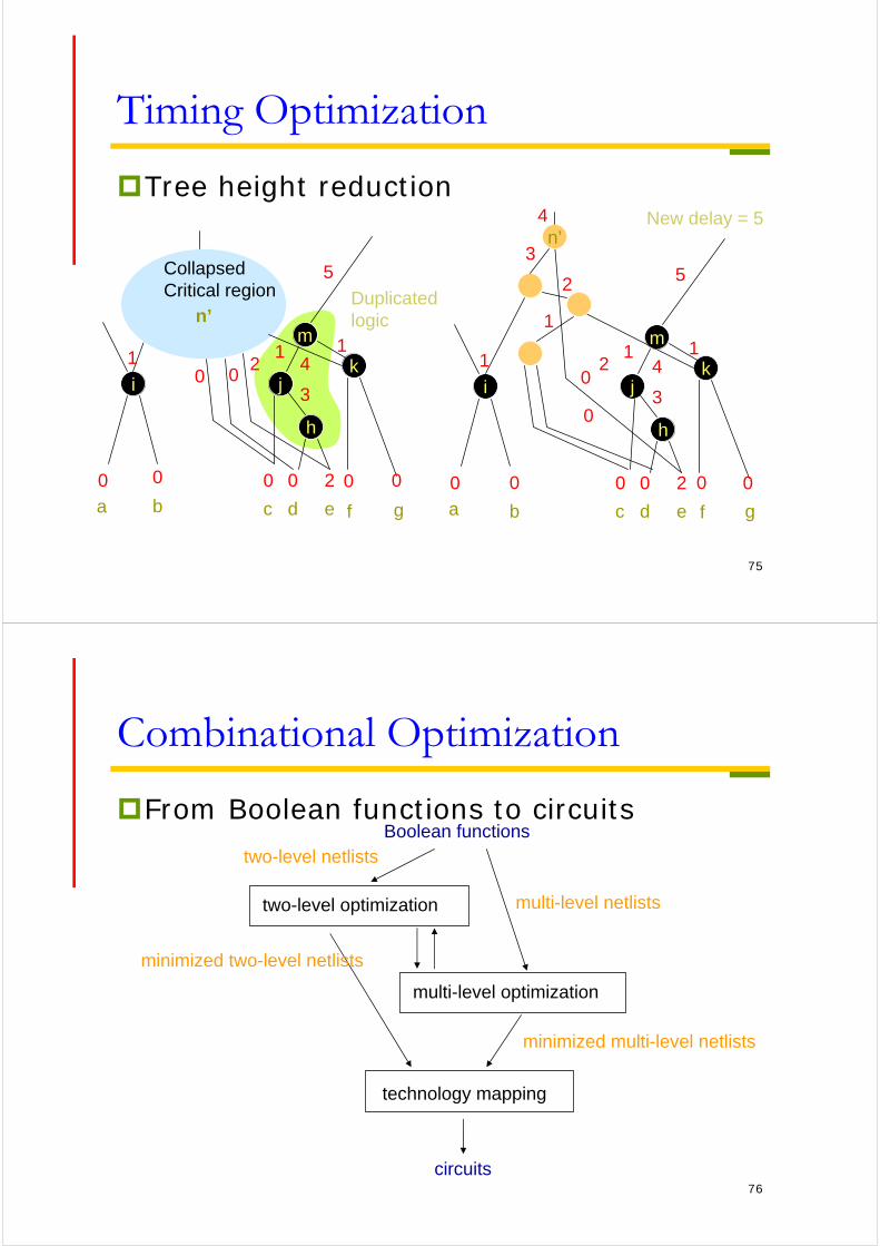
Timing Optimization
Tree height reduction
n
l m
i j
h
k
3
6
5 5
1 4
1
0 0 0 0 2 0 0
a b c d e f g
i
1
0 0a b
m
j
h
k
3
41
0 0 2 0 0
c d e f g
n’duplicatedlogic
12
00
5critical regioncollapsed
critical region
75
Timing Optimization
Tree height reduction
i
1
0 0
a b
m
j
h
k
3
41
0 0 2 0 0
c d e f g
n’Duplicatedlogic
12
00
5
i
1
0 0
a b
m
j
h
k
3
41
0 0 2 0 0
c d e f g
12
0
35
n’
2
1
0
4
CollapsedCritical region
New delay = 5
76
Combinational Optimization
From Boolean functions to circuitsBoolean functions
two-level optimization
multi-level optimization
technology mapping
circuits
two-level netlists
multi-level netlists
minimized two-level netlists
minimized multi-level netlists

77
Technology Independent vs. Dependent Optimization
Technology independent optimization produces a two-level or multi-level netlist where literal and/or cube counts are minimized
Given the optimized netlist, its logic gates are to be implemented with library cells
The process of associating logic gates with library cells is technology mapping Translation of a technology independent representation
(e.g. Boolean networks) of a circuit into a circuit for a given technology (e.g. standard cells) with optimal cost
78
Technology Mapping
Standard-cell technology mapping: standard cell design Map a function to a limited set of pre-designed library cells
FPGA technology mapping Lookup table (LUT) architecture:
E.g., Lucent, Xilinx FPGAs Each lookup table (LUT) can implement all logic functions with up to k inputs (k = 4, 5, 6)
Multiplexer-based technology mapping: E.g., Actel FPGA Logic modules are constructed with multiplexers
79
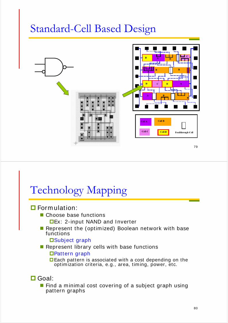
Standard-Cell Based Design
80
Technology Mapping
Formulation: Choose base functions
Ex: 2-input NAND and Inverter Represent the (optimized) Boolean network with base
functionsSubject graph
Represent library cells with base functionsPattern graphEach pattern is associated with a cost depending on the
optimization criteria, e.g., area, timing, power, etc.
Goal: Find a minimal cost covering of a subject graph using
pattern graphs
81
Technology Mapping
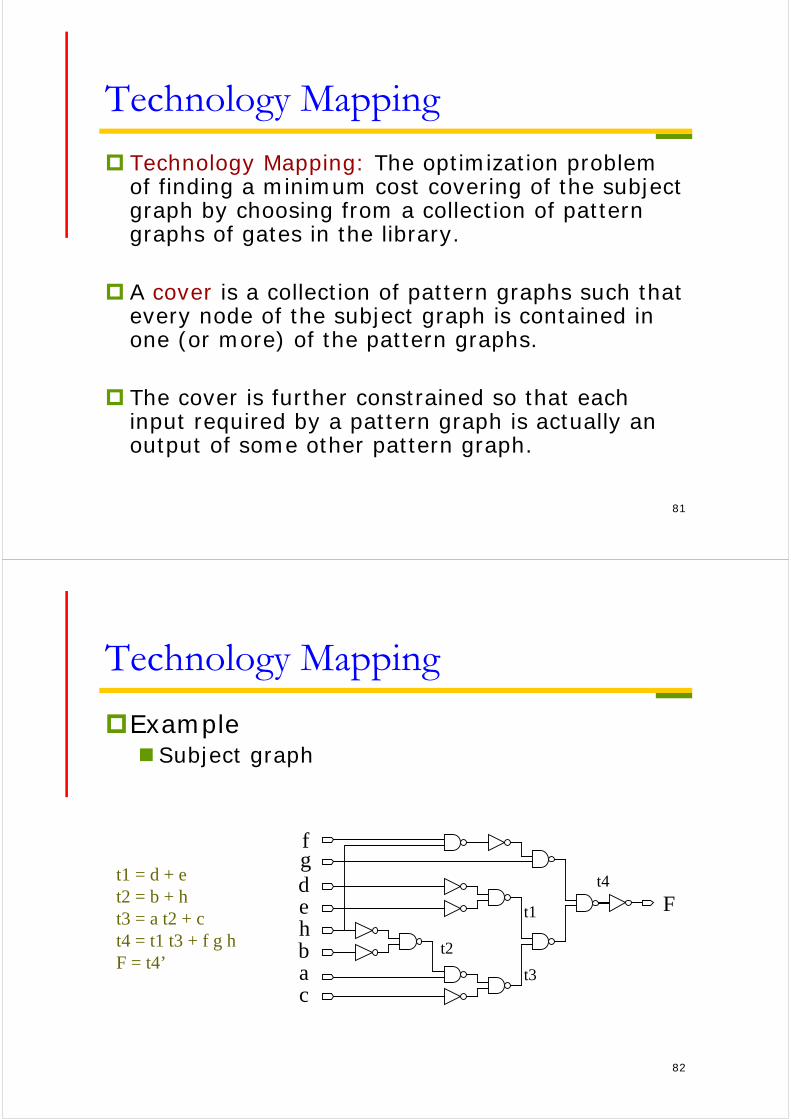
Technology Mapping: The optimization problem of finding a minimum cost covering of the subject graph by choosing from a collection of pattern graphs of gates in the library.
A cover is a collection of pattern graphs such that every node of the subject graph is contained in one (or more) of the pattern graphs.
The cover is further constrained so that each input required by a pattern graph is actually an output of some other pattern graph.
82
Technology Mapping
ExampleSubject graph
t1 = d + et2 = b + ht3 = a t2 + ct4 = t1 t3 + f g hF = t4’
fgdehbac
Ft1
t2
t3
t4
83
Technology Mapping
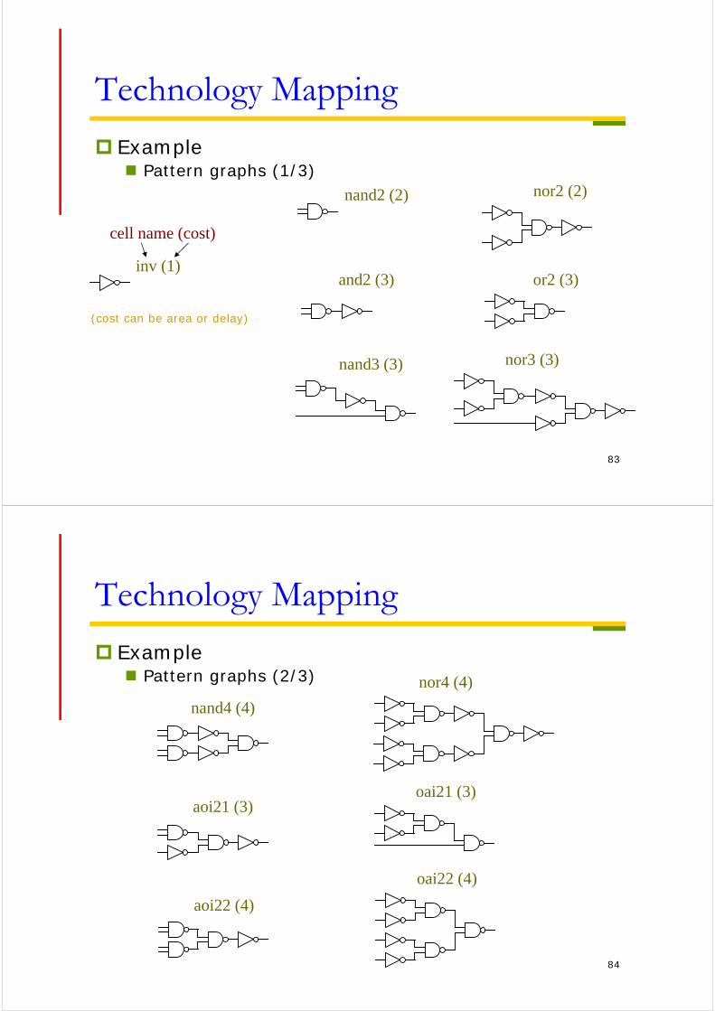
Example Pattern graphs (1/3)
inv (1)
nand2 (2) nor2 (2)
nand3 (3) nor3 (3)
cell name (cost)
and2 (3) or2 (3)
(cost can be area or delay)
84
Technology Mapping
Example Pattern graphs (2/3)
nand4 (4)
nor4 (4)
aoi21 (3)oai21 (3)
aoi22 (4)
oai22 (4)

85
Technology Mapping
Example Pattern graphs (3/3)
xor (5) xnor (5)
nand4 (4) nor4 (4)
86
Technology Mapping
Example A trivial covering
Mapped into NAND2’s and INV’s 8 NAND2’s and 7 INV’s at cost of 23
cost = 23

87
Technology Mapping
Example A better covering
fgdehbac
FOR2
OR2
AND2
AOI22
NAND2
NAND2INV
cost = 18
For a covering to be legal, every input of a pattern graph must be the output of another pattern graph!
88
Technology Mapping
Example An even better covering
OAI21OAI21
NAND3
AND2
NAND2INV
fgdehbac
F
cost = 15
For a covering to be legal, every input of a pattern graph must be the output of another pattern graph!
89
Technology Mapping
Complexity of covering on directed acyclic graphs (DAGs)
NP-complete
If the subject graph and pattern graphs are
trees, then an efficient algorithm exists (based
on dynamic programming)
90
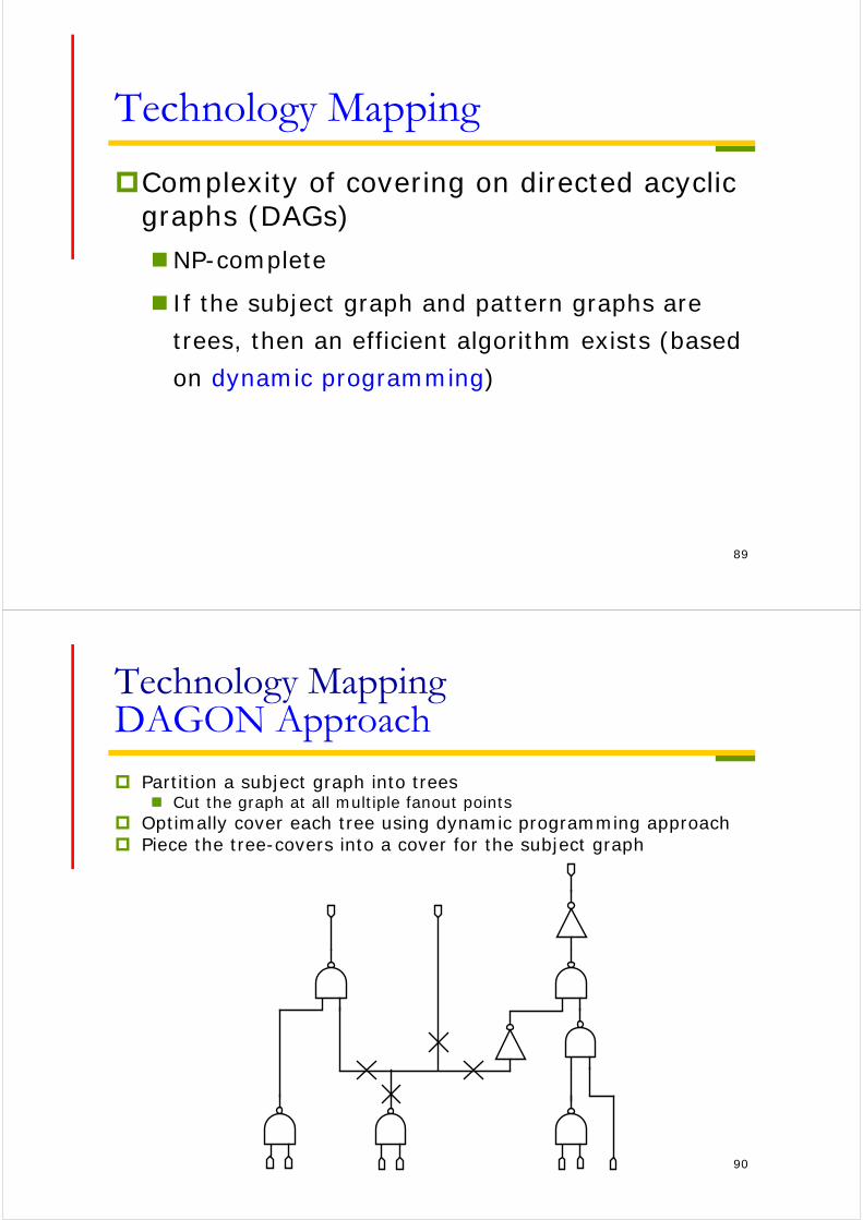
Technology MappingDAGON Approach
Partition a subject graph into trees Cut the graph at all multiple fanout points
Optimally cover each tree using dynamic programming approach Piece the tree-covers into a cover for the subject graph
91
Technology MappingDAGON Approach
Principle of optimality: optimal cover for the tree consists of a match at the root plus the optimal cover for the sub-tree starting at each input of the match
I1
I3
I2
I4
Match: cost = m
root
C(root) = m + C(I1) + C(I2) + C(I3) + C(I4) cost of a leaf (i.e. primary input) = 0
92
Technology MappingDAGON Approach
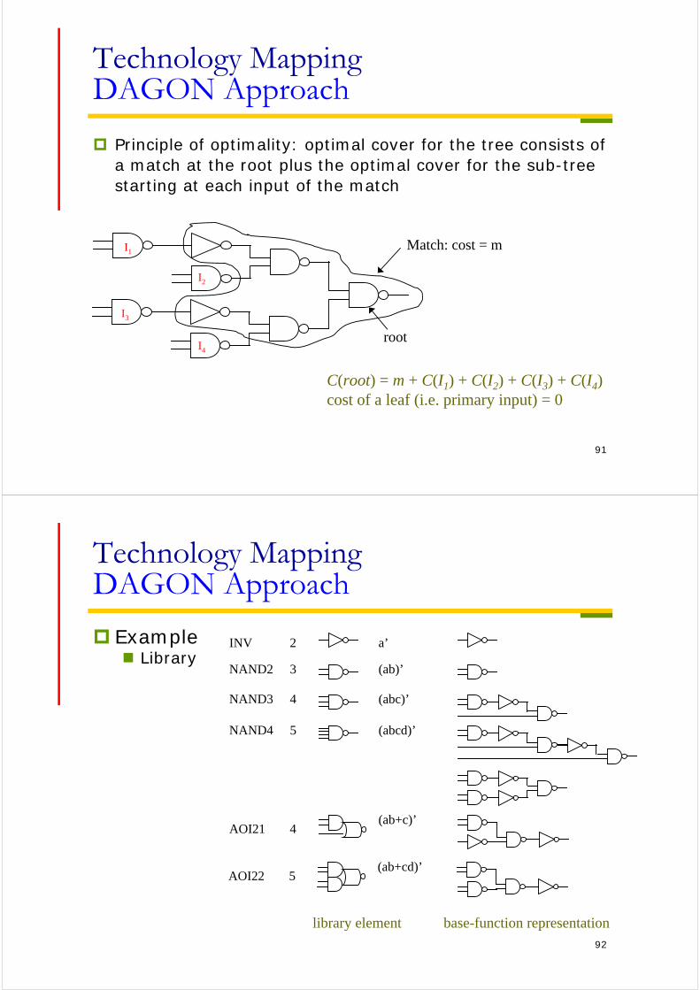
Example Library
INV 2 a’
NAND2 3 (ab)’
NAND3 4 (abc)’
NAND4 5 (abcd)’
AOI21 4(ab+c)’
AOI22 5(ab+cd)’
library element base-function representation
93
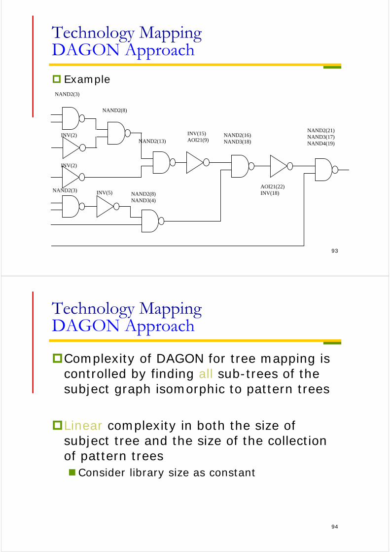
Technology MappingDAGON Approach
ExampleNAND2(3)
INV(2)
NAND2(8)
INV(2)
NAND2(3) INV(5) NAND2(8)NAND3(4)
NAND2(13)
INV(15)AOI21(9)
NAND2(16)NAND3(18)
AOI21(22)INV(18)
NAND2(21)NAND3(17)NAND4(19)
94
Technology MappingDAGON Approach
Complexity of DAGON for tree mapping is controlled by finding all sub-trees of the subject graph isomorphic to pattern trees
Linear complexity in both the size of subject tree and the size of the collection of pattern treesConsider library size as constant
95
Technology MappingDAGON Approach
Pros: Strong algorithmic
foundation Linear time complexity
Efficient approximation to graph-covering problem
Give locally optimal matches in terms of both area and delay cost functions
Easily “portable” to new technologies
Cons: With only a local (to the
tree) notion of timingTaking load values into
account can improve the results
Can destroy structures of optimized networksNot desirable for well-
structured circuits Inability to handle non-
tree library elements (XOR/XNOR)
Poor inverter allocation
96
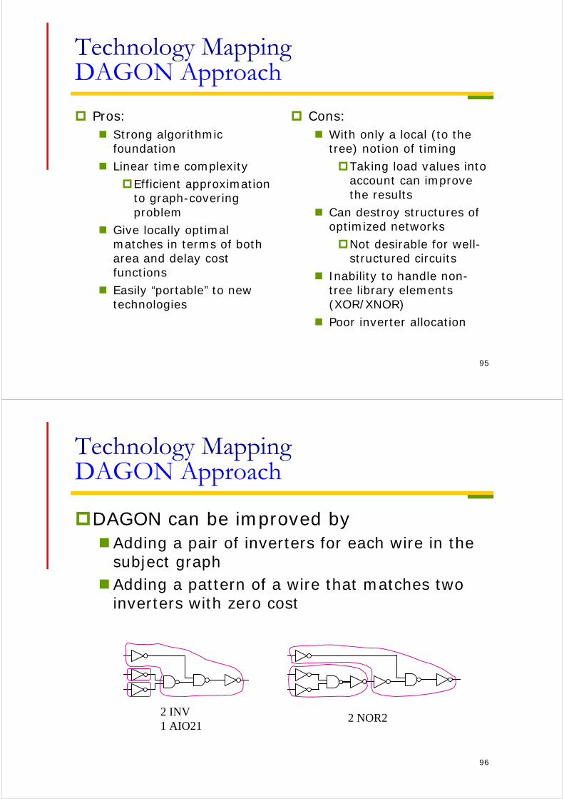
Technology MappingDAGON Approach
DAGON can be improved byAdding a pair of inverters for each wire in the
subject graphAdding a pattern of a wire that matches two
inverters with zero cost
2 INV1 AIO21
2 NOR2
97
Available Logic Synthesis Tools
Academic CAD tools: Espresso (heuristic two-level minimization, 1980s) MIS (multi-level logic minimization, 1980s) SIS (sequential logic minimization, 1990s) ABC (sequential synthesis and verification system,
2005-)http://www.eecs.berkeley.edu/~alanmi/abc/