Lec 3 ELG4179 - site.uottawa.casloyka/elg4179/Lec_3_ELG4179.pdfLecture 3 20-Sep-17 7(18) An...
19
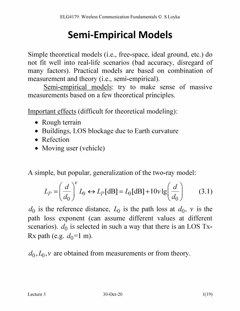
ELG4179: Wireless Communication Fundamentals © S.Loyka Lecture 3 30-Oct-20 1(19) Semi-Empirical Models Simple theoretical models (i.e., free-space, ideal ground, etc.) do not fit well into real-life scenarios (bad accuracy, disregard of many factors). Practical models are based on combination of measurement and theory (i.e., semi-empirical). Semi-empirical models: try to make sense of massive measurements based on a few theoretical principles. Important effects (difficult for theoretical modeling): • Rough terrain • Buildings, LOS blockage due to Earth curvature • Refection • Moving user (vehicle) A simple, but popular, generalization of the two-ray model: 0 0 0 0 [dB] [dB] 10 lg v P P d d L L L L v d d = ↔ = + (3.1) 0 d is the reference distance, 0 L is the path loss at 0 d , v is the path loss exponent (can assume different values at different scenarios). 0 d is selected in such a way that there is an LOS Tx- Rx path (e.g. 0 d =1 m). 0 0 , , d L v are obtained from measurements or from theory.
Transcript of Lec 3 ELG4179 - site.uottawa.casloyka/elg4179/Lec_3_ELG4179.pdfLecture 3 20-Sep-17 7(18) An...
ELG4179: Wireless Communication Fundamentals © S.Loyka
Lecture 3 30-Oct-20 1(19)
Semi-Empirical Models Simple theoretical models (i.e., free-space, ideal ground, etc.) do
not fit well into real-life scenarios (bad accuracy, disregard of
many factors). Practical models are based on combination of
measurement and theory (i.e., semi-empirical).
Semi-empirical models: try to make sense of massive
measurements based on a few theoretical principles.
Important effects (difficult for theoretical modeling):
• Rough terrain
• Buildings, LOS blockage due to Earth curvature
• Refection
• Moving user (vehicle)
A simple, but popular, generalization of the two-ray model:
0 0
0 0
[dB] [dB] 10 lg
v
P P
d dL L L L v
d d
= ↔ = +
(3.1)
0d is the reference distance, 0L is the path loss at 0d , v is the
path loss exponent (can assume different values at different
scenarios). 0d is selected in such a way that there is an LOS Tx-
Rx path (e.g. 0d =1 m).
0 0, ,d L v are obtained from measurements or from theory.

ELG4179: Wireless Communication Fundamentals © S.Loyka
Lecture 3 30-Oct-20 2(19)
Equivalently, the received power rP is:
00 0
0
[dBm] [dBm] 10 lgv
r r r r
d dP P P P v
d d
= ↔ = +
(3.1a)
where 0rP is the Rx power at reference distance 0d .
Example: 2v = for free space; 4v = for ideal ground (2-ray
model). In practice, 2 8v≤ ≤ .
Q.: find 0L , 0rP for free-space and two-ray models.

ELG4179: Wireless Communication Fundamentals © S.Loyka
Lecture 3 30-Oct-20 3(19)
Okumura-Hata Model
Correction factors are introduced to account for:
• Terrain profile (urban/suburban, rural, hilly etc.) • Antenna heights • Building profiles (height, type, concentration) • Street shape/orientation • Lakes
Okumura-Hata model is a very popular one.
• Generalization of Okumura measurements (1968) by Hata
(analytical presentation of graphs) (1980).
• Predicts average (median) path loss (attenuation).
• Terrain profile is taken into account
P.M. Shankar, Introduction to Wireless Systems, Wiley, 2002.

ELG4179: Wireless Communication Fundamentals © S.Loyka
Lecture 3 30-Oct-20 4(19)
Average (median) path loss in urban areas:
( ) 69.55 26.16lg( )
(44.9 6.55lg ) lg( )
13.85lg ( )
p
b
b mu
L dB f
h d
h a h
= + +
−
− −
(3.2)
where: f is the carrier frequency (MHz);
d is the distance (km);
bh is the BS antenna height (m) (effective);
muh is the MU antenna height (m) (above ground);
)(muha is the correction factor;
The correction factor ( )mu
a h is
2
2
3.2(lg(11.75 )) 4.97, large city, 300
( ) 8.29(lg(1.54 )) 1.1, large city, 300
(1.1 lg( ) 0.7) (1.56lg 0.8), small and medium
mu
mu mu
mu
h f MHz
a h h f MHz
f h f
− ≥
= − < ⋅ − − −
(3.3)
Limits of validity:
150 1500( )
30 200( )
1 20( )
1 10( )
b
mu
f MHz
h m
d km
h m
≤ ≤
≤ ≤
≤ ≤
≤ ≤
(3.4)
ELG4179: Wireless Communication Fundamentals © S.Loyka
Lecture 3 30-Oct-20 5(19)
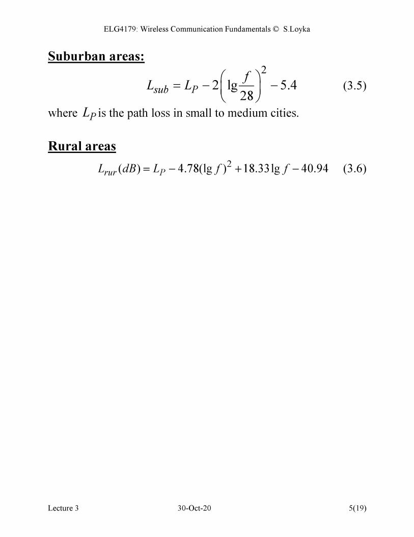
Suburban areas: 2
2 lg 5.428
sub P
fL L
= − −
(3.5)
where PL is the path loss in small to medium cities.
Rural areas
2( ) 4.78(lg ) 18.33lg 40.94rur P
L dB L f f= − + − (3.6)
ELG4179: Wireless Communication Fundamentals © S.Loyka
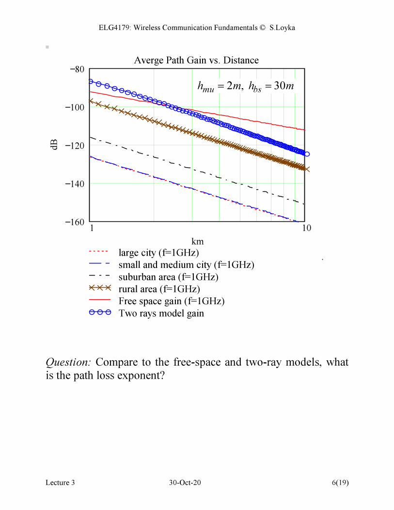
Lecture 3 30-Oct-20 6(19)
Question: Compare to the free-space and two-ray models, what
is the path loss exponent?
1 10160
140
120
100
80
large city (f=1GHz)
small and medium city (f=1GHz)
suburban area (f=1GHz)
rural area (f=1GHz)
Free space gain (f=1GHz)
Two rays model gain
Averge Path Gain vs. Distance
km
dB
.
2 , 30mu bsh m h m= =

ELG4179: Wireless Communication Fundamentals © S.Loyka
Lecture 3 30-Oct-20 7(19)
An Extension
Cost-231 extension of the Hata model:
( ) 46.3 33.93lg 13.82lg ( )
(44.9 6.55lg )lg
P b mu
b
L dB f h a h
h d c
= + − − +
− +
(3.7)
where c is a correction factor :
0 , medium city and suburban areas
3 , metropolitan areas
dBc
dB
=
Limits: the same as for the Hata model, except for
MHzf 20001500 ≤≤ .
Major limitation of the 2 models above: kmd 1≥
The model does not take into account building’s profile, street
type/orientation etc.
Many other models are available.
ELG4179: Wireless Communication Fundamentals © S.Loyka
Lecture 3 30-Oct-20 8(19)
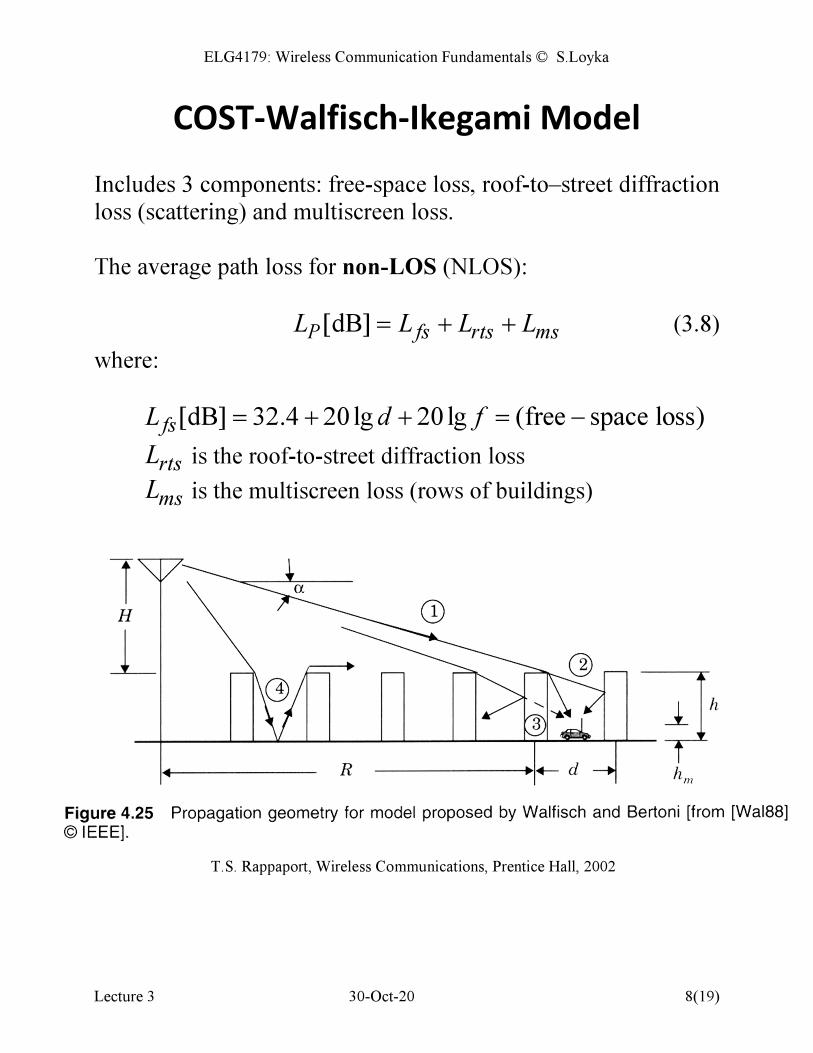
COST-Walfisch-Ikegami Model Includes 3 components: free-space loss, roof-to–street diffraction
loss (scattering) and multiscreen loss.
The average path loss for non-LOS (NLOS):
[dB]P fs rts msL L L L= + + (3.8)
where:
[dB] 32.4 20lg 20lg (free space loss)fsL d f= + + = −
rtsL is the roof-to-street diffraction loss
ms
L is the multiscreen loss (rows of buildings)
T.S. Rappaport, Wireless Communications, Prentice Hall, 2002
ELG4179: Wireless Communication Fundamentals © S.Loyka
Lecture 3 30-Oct-20 9(19)
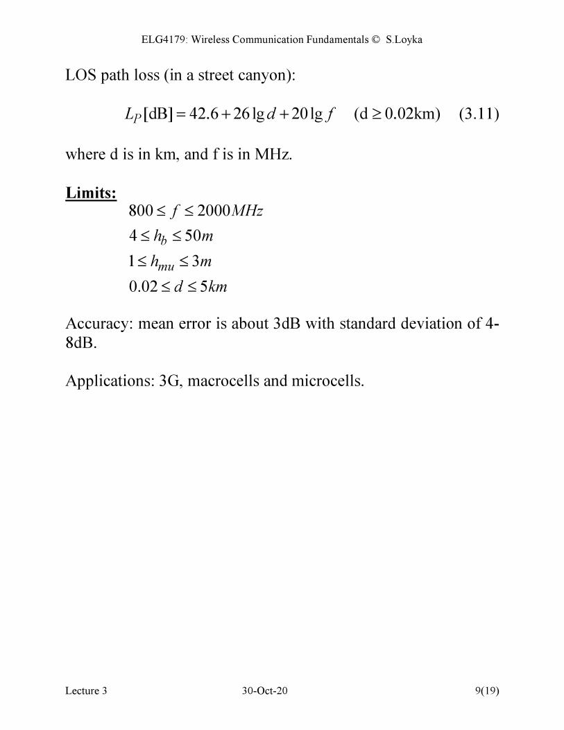
LOS path loss (in a street canyon):
[dB] 42.6 26 lg 20lg (d 0.02km)PL d f= + + ≥ (3.11)
where d is in km, and f is in MHz.
Limits:
800 2000
4 50
1 3
0.02 5
b
mu
f MHz
h m
h m
d km
≤ ≤
≤ ≤
≤ ≤
≤ ≤
Accuracy: mean error is about 3dB with standard deviation of 4-
8dB.
Applications: 3G, macrocells and microcells.
ELG4179: Wireless Communication Fundamentals © S.Loyka
Lecture 3 30-Oct-20 10(19)
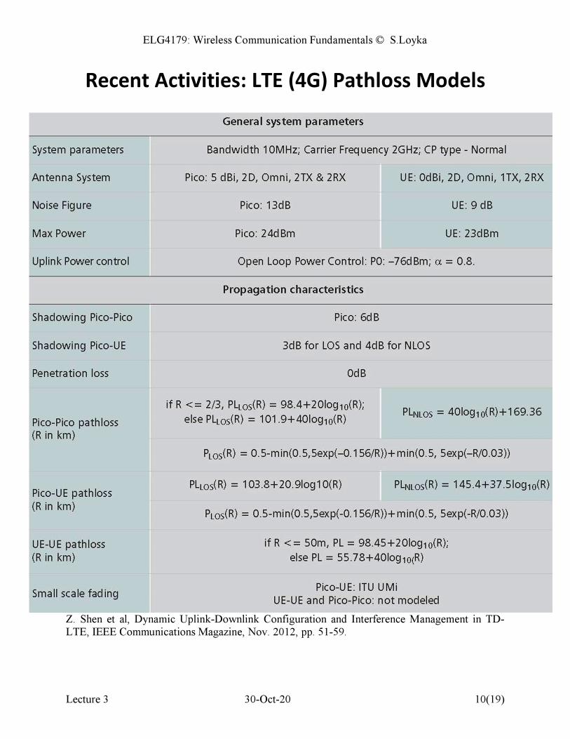
Recent Activities: LTE (4G) Pathloss Models
Z. Shen et al, Dynamic Uplink-Downlink Configuration and Interference Management in TD-LTE, IEEE Communications Magazine, Nov. 2012, pp. 51-59.
ELG4179: Wireless Communication Fundamentals © S.Loyka
Lecture 3 30-Oct-20 11(19)
Recent Activities: 5G & related models
1. T. S. Rappaport et al., “Overview of millimeter wave
communications for fifth-generation (5G) wireless networks —
with a focus on propagation models,” IEEE Trans. Antennas
Propag., vol. 65, no. 12, pp. 6213–6230, Dec. 2017.
2. S. Sun et al., “Investigation of prediction accuracy, sensitivity,
and parameter stability of large-scale propagation path loss
models for 5G wireless communications,” IEEE Trans. Veh.
Techl., vol. 65, no. 5, pp. 2843–2860, May 2016.
3. S. Sun, T.S. Rappaport, et al, Propagation Models and
Performance Evaluation for 5G Millimeter-Wave Bands, IEEE
Trans. Veh. Tech., vol. 67, no. 9, pp. 8422-8439, Sep. 2018.
4. K. Briggs, A. Shojaeifard, Coverage Regions Under Multi-
Slope Pathloss Propagation, IEEE Trans. Veh. Tech., vol. 69, no.
10, pp. 11786-11789, Oct. 2020.
5. Study on Channel Model for Frequencies from 0.5 to 100
GHz (Release 16), TR 38.901, 3GPP, Sophia Antipolis, France,
2019.
ELG4179: Wireless Communication Fundamentals © S.Loyka
Lecture 3 30-Oct-20 12(19)
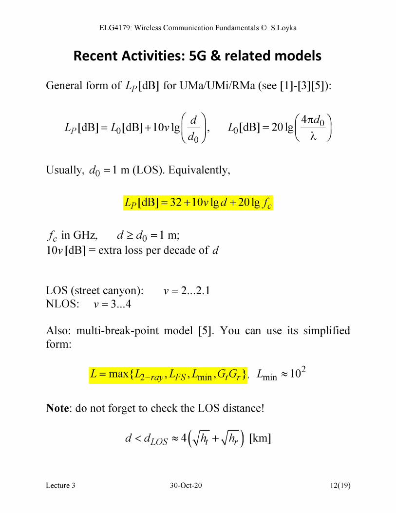
Recent Activities: 5G & related models
General form of [dB]PL for UMa/UMi/RMa (see [1]-[3][5]):
0
0
[dB] [dB] 10 lgP
dL L v
d
= +
, 0
0
4[dB] 20 lg
dL
π =
λ
Usually, 0 1d = m (LOS). Equivalently,
[dB] 32 10 lg 20 lgP cL v d f= + +
cf in GHz, 0 1d d≥ = m;
10v [dB] = extra loss per decade of d
LOS (street canyon): 2...2.1v =
NLOS: 3...4v =
Also: multi-break-point model [5]. You can use its simplified
form:
2 minmax{ , , , }ray FS t rL L L L G G−
= , 2
min 10L ≈
Note: do not forget to check the LOS distance!
( )4 [km]LOS t rd d h h< ≈ +
ELG4179: Wireless Communication Fundamentals © S.Loyka
Lecture 3 30-Oct-20 13(19)
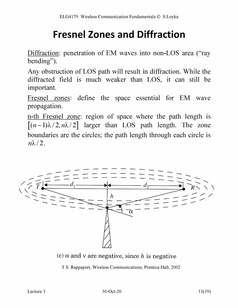
Fresnel Zones and Diffraction Diffraction: penetration of EM waves into non-LOS area (“ray
bending”).
Any obstruction of LOS path will result in diffraction. While the
diffracted field is much weaker than LOS, it can still be
important.
Fresnel zones: define the space essential for EM wave
propagation.
n-th Fresnel zone: region of space where the path length is
[ ]( 1) / 2, / 2n n− λ λ larger than LOS path length. The zone
boundaries are the circles; the path length through each circle is
/ 2nλ .
T.S. Rappaport, Wireless Communications, Prentice Hall, 2002

ELG4179: Wireless Communication Fundamentals © S.Loyka
Lecture 3 30-Oct-20 14(19)
Fresnel zone radius:
21
21
dd
ddnrn
+
=
λ (3.12)
where nrdd >>
21, .
Diffraction and Fresnel zones can be explained using Huygen’s
principle (secondary sources).
Contribution of each successive zone is less than the previous
one. Blockage of some zones results in diffraction.
Area essential for EM wave propagation
There is no disturbance to the wave propagation along a certain
path provided that 1st Fresnel zone is cleared.
Rule of thumb for LOS microwave link design: ~50% of 1st zone
must be kept clear.
ELG4179: Wireless Communication Fundamentals © S.Loyka
Lecture 3 30-Oct-20 15(19)
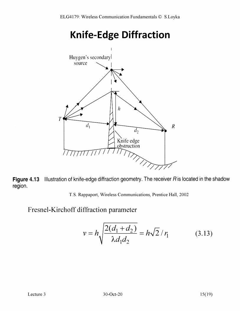
Knife-Edge Diffraction
Fresnel-Kirchoff diffraction parameter
1 2
1
1 2
2( )2 /
d dv h h r
d d
+= =
λ (3.13)
T.S. Rappaport, Wireless Communications, Prentice Hall, 2002

ELG4179: Wireless Communication Fundamentals © S.Loyka
Lecture 3 30-Oct-20 16(19)
The field is given by Fresnel integral
2
0
1( ) exp( / 2)
2v
E jF v j t dt
E
∞
+= = − π∫ (3.14)
where 0
E is the LOS field (no obstruction).
The field has oscillating behavior w.r.t. h. This is a simple model
(approximation). Yet, it is good enough to model many obstacles
(buildings, mountains, etc.). Generalizations are possible:
multiple knife-edge models.
Another representation: introduce Fresnel integrals,
2 2
0 0
( ) cos , S( ) sin2 2
x x
C x t dt x t dtπ π
= =
∫ ∫ (3.15)
Then,
[ ]1 1
( ) ( ) ( )2 2
jF C jS
+ν = − ν − ν (3.16)
Note that 12
( ) ( )C S∞ = ∞ = .
The total path loss is
0p dL L L= (3.17)
where 2
0 (4 / )L R= π λ is the free-space path loss,
2
( )dL F−
= ν is the diffraction loss.

ELG4179: Wireless Communication Fundamentals © S.Loyka
Lecture 3 30-Oct-20 17(19)
An Approximation1
If 1 2,d d h>> >> λ :
2
2 1 2
2 20 1 2
1( )
4d
E d dF
L E d dh
λ= ν = ≈
+π
Note: if the edge is not sharp but rounded, expect 10-20 dB
more loss.
1 see Kraus, Fleish, Electromagnetics with Applications, 5th Edition, McGraw Hill, 1999. (p.235-236).
ELG4179: Wireless Communication Fundamentals © S.Loyka
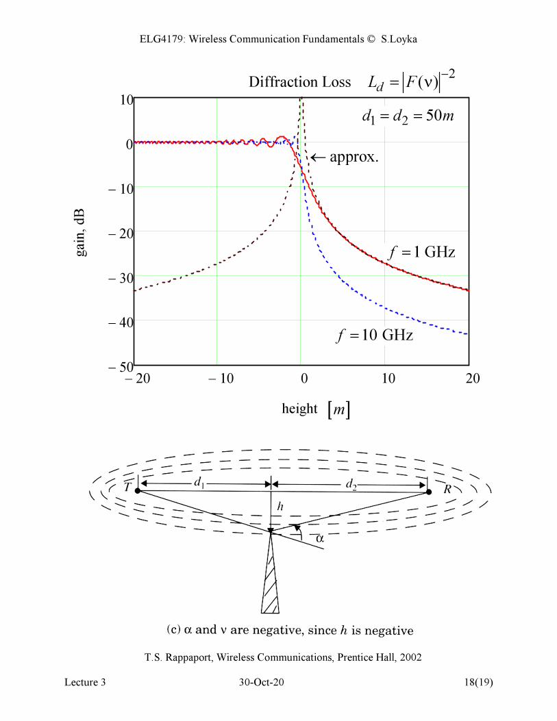
Lecture 3 30-Oct-20 18(19)
20− 10− 0 10 2050−
40−
30−
20−
10−
0
10
Diffraction Loss
height
gai
n, dB
1 2 50d d m= =
T.S. Rappaport, Wireless Communications, Prentice Hall, 2002
[ ]m
1 GHzf =
10 GHzf =
2( )dL F
−
= ν
approx.←
ELG4179: Wireless Communication Fundamentals © S.Loyka
Lecture 3 30-Oct-20 19(19)
Summary
• Average (median) path loss. Semi-empirical models.
• Okumura-Hata model. Extension to PCS environments.
• COST-Walfisch-Ikegami Model.
• Fresnel zones and diffraction. Knife-edge diffraction.
Reading:
o Rappaport, Ch. 4.
References:
o S. Salous, Radio Propagation Measurement and Channel
Modelling, Wiley, 2013. (available online)
o J.S. Seybold, Introduction to RF propagation, Wiley, 2005.
o Other books (see the reference list).
Note: Do not forget to do end-of-chapter problems. Remember
the learning efficiency pyramid!