Lebesgue Measure on The Real Numbers ℝ

And Lebesgue Theorem on Riemann Integrability

By Ng Tze Beng

In this article, we shall construct the Lebesgue measure on the set of real numbers ℝ . We

shall do this via a set function on the collection of all subsets of ℝ . This set function is

called the outer measure on ℝ . We shall show that the Lebesgue measure is translation

invariant and that on interval I, it is equal to the length of I. We shall characterize Riemann

integrability in terms of measure theoretic property.

Definition 1. Let I be an interval with end points a and b with a < b. The length ( )I is

defined by ( )I b a . If I is an unbounded interval, then define ( )I .

We want to extend this notion of length to arbitrary subsets of ℝ .

Let be the family of all countable collections of open intervals. Define

* : ℝ ,

by *( ) ( )I

I

for any . Hence, 0 *( ) . Note that as each ( )I is non-

negative, the summation ( )I

I

is absolutely convergent (including ∞) and does not depend

on the order of summation.

Suppose is a collection of open intervals and V is a subset of ℝ . We say is a covering

for V or covers V if I

V I

∪ .

Now, let E be an arbitrary subset of ℝ . Let ( ) : covers C E E . Note that C(E)

. Define *( ) inf *( ) : ( )E C E ℝ . This is called the Lebesgue outer measure

of E. We have thus defined a function from the set of all subsets of ℝ into ℝ ,

*: P ( )ℝ = 2ℝ ℝ .

Then we have:

Proposition 2.

(i) *() = 0.

(ii) *({ }) 0x for all xℝ .

2

(iii) For any two subsets A and B of ℝ , *( ) *( )A B A B .

Proof.

(i) and (ii)

Take xℝ . Then for any integer n ≥ 1, the open interval 1 1

,x xn n

covers {x}.

Therefore, 1 1 2

*({ }) ,x x xn n n

. Since 2

0n , *({ }) 0x .

As { }x , 1 1

{ } ,x x xn n

, *( ) 0 .

(iii) Suppose A B . Then any countable cover of B is also a countable cover of A.

Hence, ( ) ( )C B C A . Therefore,

*( ) inf *( ) : ( ) inf *( ) : ( ) *( )B C B C A A .

Let rℝ . Let :r ℝ ℝ be the translation map given by ( )r x x r for xℝ .

The next result gives the desirable property of the Lebesgue outer measure on ℝ . It is

translation invariant. Not all outer measures need to be translation invariant but for a

generalization of length on subsets of ℝ , translation invariant is expected as the translated

interval is still an interval and the length of the interval does not change after the translation.

Proposition 3. For any rℝ , * ( ) *r E E for any subset E of ℝ .

Proof.

If I is an open interval with endpoints a < b, then ( )r I is an open interval with end points a

+r and b+r . Hence, ( )r I I b a . For every , let

( ) ( ) :r r I I .

Suppose E is a subset of ℝ .

If covers E, then plainly, ( )r covers ( )r E . Observe that

* ( ) ( ) *r r

I I

I I

.

3

It follows that *( ) : ( ) * ( ) : ( ) * : ( )r rC E C E C E .

Hence, * ( ) inf *( ) : ( ) inf *( ) : *r rE C E C E E .

As ( )r r E E , by applying the above inequality with ( )r E in place of E and r in

place of r , we get *( ) * ( ) * ( )r r rE E E . Hence * ( ) *r E E .

Next, we show that the outer measure does extend the meaning of length of an interval.

Proposition 4. For any interval I, *( ) ( )I I .

Proof. We shall establish the proposition for closed and bounded interval I = [a, b] with a <

b. Now, , ( , )a b a b for any > 0 and so *( ) ( , ) 2I a b b a . As

is arbitrary, we have that *( ) ( )I b a I . We want to show that for every in C(I),

*( ) b a . Since [a, b] is compact, every open covering in C(I), has a finite sub-

covering, say , then *( ) *( ) . So, we now assume that is a finite collection of

open intervals that cover I.

Starting with a, since covers I, there is an open interval 1 1( , )a b in such that 1 1( , )a a b ,

i.e., 1 1a a b . If 1b b , then 1 1 1 1*( ) ( , )a b b a b a . If 1b b , then 1b I

and there exists an open interval 2 2( , )a b in such that 1 2 2( , )b a b with 2 1 2a b b . If

2b b , then

1 1 2 2 1 1 2 2 1 2 2 1( , ) ( , )a b a b b a b a b a b b a a a b b a .

Since is a finite collection, this process of covering the end point of the next interval must

terminate. Suppose it terminate at the n-th interval ( , )n na b such that nb b and n ≥ 2.

Then we have 1k k ka b b , where we have denoted 0b a for k =1, 2, …., n1. Hence, we

have

1 1 1

1 1 2

*( ) ( , )n n n

i i i i i i n n

i i i

a b b a b a b a b a b a

.

Therefore, *( ) inf *( ) : ( )I C I b a and so *( ) ( )I b a I .

Now let I be any bounded interval with end points a, b with a < b. For any 04

b a

,

, ,a b I a b . Then by Proposition 2 (iii),

* , * * ,a b I a b .

4

It follows that 2 *b a I b a . Therefore, as is arbitrary, * ( )I b a I .

Finally, let I be an unbounded interval. Then for any real number K > 0, the interval I

contains a bounded interval H of length ( )H K . Therefore, *( ) *( )I H K . It

follows that *( ) ( )I I .

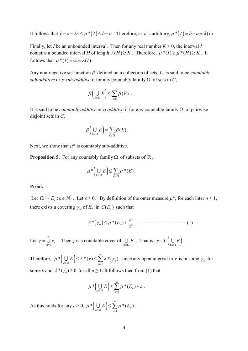
Any non-negative set function defined on a collection of sets, C, is said to be countably

sub-additive or sub-additive if for any countably family of sets in C,

( )E E

E E

∪ .

It is said to be countably additive or additive if for any countable family of pairwise

disjoint sets in C,

( )E E

E E

∪ .

Next, we show that * is countably sub-additive.

Proposition 5. For any countably family of subsets of ℝ ,

* *( )E E

E E

∪ .

Proof.

Let :nE n ℕ . Let > 0. By definition of the outer measure *, for each inter n ≥ 1,

there exists a covering n of En in ( )

nC E such that

* *( )2

n n nE

. ---------------------------- (1)

Let 1

nn

∪ . Then is a countable cover of

E

E∪ . That is,

E

C E

∪ .

Therefore, 1

* *( ) *( )nE n

E

∪ , since any open interval in is in some k for

some k and *( ) 0n for all n ≥ 1. It follows then from (1) that

1

* *( )nE n

E E

∪ .

As this holds for any > 0, 1

* *( )nE n

E E

∪ .

5

Corollary 6. If E is a countable subset of ℝ , then *( ) 0E .

Proof. Suppose E is countable subset of ℝ and so 1

nn

E x

∪ . Then

1 1

*( ) * * 0n nn i

E x x

∪ by Proposition 5 and Proposition 2(ii).

Hence, *( ) 0E .

As a consequence,

Corollary 7. Every interval is not countable.

The Lebesgue outer measure on ℝ is countably sub-additive on the collection of all subsets

of ℝ but not countably additive. In order to obtain a countably additive function from it, we

restrict the domain to a subset of the power set of ℝ . In this procedure, we follow

Caratheodory’s restriction method, we call the restricted collection, the Lebesgue measurable

subsets of ℝ or the Lebesgue measure on ℝ .

A subset E of ℝ is said to be Lebesgue measurable if, and only if, for any subset X of ℝ , we

have,

*( ) *( ) *( )X X E X E .

Since ( )X X E X E , we have by Proposition 5 that for any subset X of ℝ ,

*( ) *( ) *( )X X E X E .

We have immediately the following:

Lemma 8. A subset E of ℝ is Lebesgue measurable if, and only if, for all X ℝ ,

*( ) *( ) *( )X X E X E .

Proposition 9. If E ℝ is Lebesgue measurable, then its complement cE E ℝ is also

Lebesgue measurable.

Proof. Note that for all X ℝ , ( )X E X E ℝ and ( )X E X E ℝ .

Proposition 9 follows from Lemma 8.

6

Observe that for any X ℝ , X and X X . Trivially we have for any

X ℝ , *( ) *( ) *( ) 0 *( ) *( )X X X X X . Thus, Ø is Lebesgue

measurable and by Proposition 9, ℝ is Lebesgue measurable. We record our conclusion as:

Proposition 10. and ℝ are Lebesgue measurable.

Proposition 11. If A and B are Lebesgue measurable subsets of ℝ , then A B is also

Lebesgue measurable.

Proof.

Since B is Lebesgue measurable, for any X ℝ ,

*( ) * ( ) * ( )X A X A B X A B .

Now ( )X A B X A X A B and so by Proposition 5,

* * * ( )X A B X A X A B .

Therefore,

* * ( ) * *( ) * ( )X A X A B X A X A X A B

* X A B .

Hence, * *( ) * ( ) * ( )X A X A X A B X A B .

But A is Lebesgue measurable and so,

*( ) * *( ) * ( ) * ( )X X A X A X A B X A B for all X ℝ .

It follows by Lemma 8 that A B is Lebesgue measurable.

Corollary 12. If A and B are Lebesgue measurable subsets of ℝ , then A B is also

Lebesgue measurable.

Proof. Note that A B A B ℝ ℝ ℝ . Since A and B are Lebesgue measurable,

by Proposition 9, and A B ℝ ℝ are Lebesgue measurable and consequently, by

Proposition 11, A B A B ℝ ℝ ℝ is Lebesgue measurable. By Proposition 9,

A B is Lebesgue measurable.

7

Let M be the set of all Lebesgue measurable subsets of ℝ .

Lemma 13. If E1, E2, …, En are pairwise disjoint Lebesgue measurable sets in M , then for

any X ℝ ,

1

1

* *nn

i ii i

X E X E

∪ .

Proof. The lemma is trivially true for n = 1.

Let n > 1. We shall prove this lemma by induction. Assume the lemma is true for a

collection of less than n members of pairwise disjoint Lebesgue measurable sets. Let X be any

subset of ℝ .

Since En is Lebesgue measurable, for any subset Y of ℝ ,

*( ) * *n nY Y E Y E . ----------------------- (1)

Take 1

n

ii

Y X E

∪ . Now, n nY E X E and as

1

n

i iE

are pairwise disjoint,

1

1

n

n ii

Y E X E

∪ . It follows from (1) that

1

1 1

* *( ) * *n n

i n ii i

X E Y X E X E

∪ ∪

and by the induction hypothesis,

1

1 1

* * *nn

i n ii i

X E X E X E

∪

1

*n

i

i

X E

.

This completes the proof.

Next, we have:

Theorem 14. Suppose 1i i

E

is a countable collection of Lebesgue measurable subsets of

ℝ , i.e., members of M , then 1

ii

E

∪ M .

Proof.

The first thing that we do is to write 1

ii

E

∪ as a disjoint union.

8

Let 1 1

S E , 2 1 2 1 2 1 2 1S E E E E E E E ℝ . For integer n ≥ 2, let

1 1

1 1

n n

n n i ni i

S E E E E

∪ ℝ ∪ .

By Proposition 11, Proposition 12 and Proposition 9, Sn is Lebesgue measurable for integer n

≥ 2.

Plainly, i iS E for all integer i ≥ 1. Therefore, 1 1

i ii i

S E

∪ ∪ . Take

1i

i

x E

∪ . Then nx E for

some integer n ≥ 1. If n =1, then 1 1nx E E S . If n > 1, then let k be the least integer

such that kx E . Then k n. If k =1, then 1 1kx E E S . If k > 1, then jx E for j k1.

Therefore, 1

1

k

k i ki

x E E S

∪ . It follows that

1 1i i

i i

E S

∪ ∪ . Hence,

1 1i i

i i

E S

∪ ∪ .

For i j, 11

1 1

ji

i j i j k kk k

S S E E E E

ℝ ∪ ℝ ∪

1

1

j

i j kk

E E E

ℝ ∪ , if i < j,

.

As i j either i < j or j < i. It follows that i jS S for i j. We conclude that 1

ii

S

∪

is a disjoint union.

Let 1 1

n

n i ii i

D S E E

∪ ∪ . Then Dn is Lebesgue measurable by Corollary 12. Therefore,

for X ℝ ,

*( ) * * * *n n nX X D X D X D X E ,

since nX E X D . It then follows by Lemma 13 that

1

*( ) * *n

i

i

X X S X E

.

Since this holds for any integer n ≥ 1, we have

1

*( ) * *i

i

X X S X E

. ---------------- (1)

But by Proposition 5 (countable sub-additivity of the outer measure),

9

1 11

* * ( ) * *i i ii ii

X S X S X S X E

∪ ∪ .

It follows from (1) that *( ) *( ) *X X E X E . Hence, by Lemma 8, 1

ii

E E

∪

is Lebesgue measurable. That is, E M .

We now state our main theorem

Theorem 15. The set M , of all Lebesgue measurable subsets of ℝ , is a -algebra and (ℝ ,

M ) is a measure space. The set function on M given by the restriction of the Lebesgue

outer measure to M , = *M : M ℝ , is a positive measure. Hence, (ℝ , M , ) is a

measure space.

M is called the Lebesgue measure on ℝ and the set function, : M ℝ is called the

Lebesgue measure.

Proof. By Proposition 9, Proposition 10 and Theorem 14, M is a -algebra and so (ℝ , M )

is a measure space. Since ( ) *( ) 0 , is non-trivial. It remains to show that is

countably additive on M .

Suppose 1i i

E

is a countable collection of pairwise disjoint Lebesgue measurable sets in M .

Then for any integer n ≥ 1, by Lemma 13, with X = ℝ , we have

1 1 1 1

* *n nn n

i i i ii i i i

E E E E

∪ ∪ .

Since 1 1

n

i ii i

E E

∪ ∪ ,

1 1 1 1 1

* * *n nn

i i i i ii i i i i

E E E E E

∪ ∪ ∪ for each n ≥

1. Therefore,

1 1

i ii i

E E

∪ .

But by Proposition 5 (countable sub-additivity),

1 1 1 1

* *i i i ii i i i

E E E E

∪ ∪ .

10

It follows that 1 1

i ii i

E E

∪ . Hence, is countably additive on M and so is a

positive measure on M .

Proposition 16. Every subset E of ℝ with *( ) 0E is Lebesgue measurable. Hence, the

-algebra M is -complete. That is the measure space (ℝ ,M , ) is a complete measure

space.

Proof.

Suppose *( ) 0E . Take any subset X of ℝ . Since X E E , by Proposition 2,

0 * *( ) 0X E E and so * 0X E . Also, as X X E ,

*( ) *( )X X E . Therefore, *( ) *( ) *( ) *( )X X E X E X E . Hence,

by Lemma 8, E is Lebesgue measurable.

Consider the -completion of M ,

M * ={E ℝ : there exists A, B M , such that A E B and ( ) 0B A }.

Note that M M *. If A, B M is such that A E B and ( ) 0B A , then since

E A B A , *( ) *( ) ( ) 0E A B A B A implies that E – A M and so

E E A A M . It follows that M * M . Therefore, M * = M and so M is -

complete.

Proposition 17. Every open subset of ℝ is Lebesgue measurable. Hence the Borel subsets

of ℝ , B is contained in the -algebra M of Lebesgue measurable subsets of ℝ . This means

B is a sub -algebra of M .

Proof. Any open subset E of ℝ is a countable union of open intervals. By Theorem 14, it is

sufficient to show that any open interval is Lebesgue measurable.

Since ( , ), ( , ) : ,a b a b ℝ is a subbase for the topology on ℝ , by Proposition 11, it is

sufficient to show that (a, ∞) and (∞, b) for any a and b in ℝ , are Lebesgue measurable.

Note that, for any subset X in ℝ , ( , ) ( , ]X a X a . If we can show that (a, ∞) is

Lebesgue measurable, then by Proposition 9, ( , ] ( , )a a ℝ is Lebesgue measurable. It

follows then that for any b in ℝ , by Theorem 14, 1

1( , ) ,

n

b bn

∪ is Lebesgue

measurable. Hence, it is sufficient to prove that (a, ∞) is Lebesgue measurable for any a in

ℝ . We shall show that for any subset X ℝ ,

*( ) *( ( , )) *( ( , ])X X a X a .

If *( )X , then we have nothing to prove and so we assume that *( )X .

11

Take any > 0. Then by the definition of the Lebesgue outer measure *, there exists a

countable covering of X by open intervals with

*( ) ( ) *( )I

I X

.

For each open interval I , each of the sets ( , ) and ( , ]I a I a is either empty or an

interval. Moreover, ( , ) ( , ]I I a I a is a disjoint union and so

( ) ( , ) ( , ] * ( , ) * ( , ]I I a I a I a I a .

As ( , ) :I a I covers ( , )X a ,

*( ( , )) * ( , )I

X a I a

∪

* ( , )I

I a

, by Proposition 5 (countable sub-additivity). -----(1)

Similarly, since ( , ] ( , ]I

X a I a

∪ ,

*( ( , ]) * ( , ]I

X a I a

∪ by Proposition 2(iii),

* ( , ]I

I a

, by Proposition 5. ---------------- (2)

It follows from (1) and (2) that

*( ( , )) *( ( , ])X a X a

* ( , ) * ( , ]I I I

I a I a I

*( )X .

Since this is true for any > 0, *( ( , )) *( ( , ]) *( )X a X a X .

This holds for any subset X ℝ , by Lemma 8, (a, ∞) is Lebesgue measurable.

This completes the proof.

In summary, we have

Theorem. (ℝ ,M , ) is a measure space such that M is -complete, is non-trivial and M

contains the Borel subsets of ℝ .

12

Next, we investigate the relation of the Lebesgue integral with the Riemann integral on a

bounded interval.

Definition 18. Suppose E is a Lebesgue measurable subset of ℝ . We say a real valued

Lebesgue measurable function :f E ℝ is Lebesgue integrable if

E

f d .

(See Definition 29, Introduction to Measure Theory.)

We recall the following result.

Theorem 19. Suppose E is a Lebesgue measurable subset of ℝ and ( )E . Suppose

:f E ℝ is bounded. Then f is measurable if, and only if, the lower and upper Lebesgue

integral of f are the same. The lower Lebesgue integral of f is defined by

sup : , ( )E E

f d d f S E and the upper Lebesgue integral of f is defined by

inf : , ( )E E

f d d f S E , where S(E) is the set of real-valued simple

measurable functions on E.

(This is Theorem 7 in Positive Borel Measure and Riesz Representation Theorem.)

Proof.

Suppose f is measurable. As f is bounded, we assume f . Let nn

, for integer

n ≥ 1. Define 1

. [ ( 1) , )n i n nE f i i for 1 i n , n = 1, 2, … .

Then ,n iE are measurable and for each integer n ≥ 1,

,

1

( )n

n ii

E E

∪ , where

,1

n

n ii

E∪ is a disjoint union,

,

1

n

n i

i

E

.

Let ,

1

( 1)n i

n

n n E

i

i

and ,

1n i

n

n n E

i

i

for each integer n ≥ 1. Thus, ,n n

are simple measurable functions on E such that

( ) ( ) ( )n nx f x x for all x in E.

Therefore,

13

,

1

( 1) ( )n

n n n iE E

i

f d d i E

and

,

1

n

n n n iE E

i

f d d i E

.

Hence, ,

1

( ) ( )n

n n i nE E

i

f d f d E E

.

But 0n as n and so E E

f d f d . SinceE E

f d f d , it follows that

E Ef d f d

Conversely, suppose E E

f d f d . We shall show that f is measurable or -measurable.

Let ( ) ( ) :L f S E f and ( ) ( ) :U f S E f . Then

sup : ( )E E

f d d L f and inf : ( )E E

f d d U f . Since f is

bounded and ( )E , E E

f d f d . Thus, for any integer n ≥ 1, there exists

( )n L f and ( )n U f such that

1

nE E

d f dn

and 1

nE E

d f dn

.

Hence, 2n n n n

E E Ed d d

n . This holds for all integer n ≥ 1.

Define , : E ℝ , by 1

sup n n

and

1inf n n

. Then both and are

measurable since each n and n are measurable for all integer n ≥ 1.

Plainly, n nf .

Let 1

: ( ) ( )kD x E x xk

.

Obviously, ,

1: ( ) ( )k n n k nD x E x x D

k

for all integer n ≥ 1.

Hence, ,

1k nD n n

k and so

,

1k nD n n

E Ed d

k . It follows that

14

,

1 2k n n n

ED d

k n .

Therefore, ,

2k k n

kD D

n for all integer n ≥ 1. It follows that 0kD .

Let : ( ) ( ) 0D x E x x . Then 1

kk

D D

∪ and

1 2 kD D D D ⋯ ⋯ .

Therefore, ( ) lim 0kk

D D

. This means almost everywhere with respect to the

Lebesgue measure . As f , f on E D and f almost everywhere

with respect to the Lebesgue measure . Since E is measurable and the Lebesgue measure is

complete, E D is measurable. Therefore, f is measurable on E D since is measurable.

Hence, f is measurable.

Theorem 20. Suppose E is a Lebesgue measurable subset of ℝ and ( )E . Suppose

:f E ℝ is a bounded measurable function. Then f is Lebesgue integrable and

E E E E E

f d f d f d f d f d .

(This is Theorem 8 in Positive Borel Measure and Riesz Representation Theorem.)

Proof.

Since :f E ℝ is measurable, max ,0f f and min ,0f f are measurable.

Thus, f f f and f f f is measurable. Note that , and f f f are

bounded non-negative functions. Then by definition,

sup : 0 , ( )E E

f d s d s f s S E

and sup : 0 , ( )E E

f d s d s f s S E .

Since both : 0 , ( )E

s d s f s S E and : 0 , ( )E

s d s f s S E are bounded

above by ( )K E for some constant K such that ( )f x K for all x in E, E

f d and

Ef d exist and are finite and so

E E Ef d f d f d . Thus, by definition, f

is Lebesgue integrable on E and

E E E

f d f d f d .

Since f is measurable,

15

sup : ( ) sup : ( ) :E E E

f d d L f d S E f

sup : ( ) : 0E E

d S E f f d .

Similarly, we have E E

f d f d . By Theorem 19, E E E

f d f d f d and

E E Ef d f d f d .

E E E Ef d f d f d f d

inf : , ( ) sup : ( ),E E

d f S E d S E f

inf : , ( ) inf : ( ),E E

d f S E d S E f

inf : , ( ) inf : ( ),E E

d f S E d S E f

inf : , ( ) inf : , ( ),E E

d f S E d f S E

inf : , , , ( )E E

d d f f S E

inf : , , , ( )E

d f f S E

inf : , ( )E E

d f f f S E f d .

Similarly,

E E E E

f d f d f d f d

sup : , ( ) inf : ( ),E E

d f S E d S E f

sup : , ( ) sup : ( ),E E

d f S E d S E f

sup : , ( ) sup : ( ),E E

d f S E d S E f

sup : , ( ) sup : ( ),E E

d f S E d S E f

16

sup : , , , ( )E E

d d f f S E

sup : , , , ( )E

d f f S E

sup : , ( )E E

d f f f S E f d .

Thus, we have E E E E

f d f d f d f d . Now, as f is measurable and

( )E , by Theorem 19, E E

f d f d and so it follows that

E E E E

f d f d f d f d .

Suppose :[ , ]f a b ℝ is bounded. A step function s on [a, b] is a function that assumes

finite constant values on the open subintervals of [a, b] defined by some partition of [a, b].

More precisely, there is a partition 0 1 2 nx a x x x b ⋯ and a set of constants,

1 2, , , n ⋯ such that ( ) is x for

1i ix x x for 1 i n. Plainly, a step function is a

simple -measurable function. We define the Riemann integral on step function s by the

expression,

1

1

( )nb b

i i ia a

i

s R s x x

.

This is the usual definition of Riemann integral on step function. Observe that as a step

function s is bounded and measurable, s is Lebesgue integrable and

0

1 1[ , ] [ , ]

1 1

( , ) ( )n

i i

n n

i i i i i ia b a b x

i i

s d s d x x x x

.

Thus, the Riemann integral of a step function and the Lebesgue integral of a step function are

the same. This is the main lead to showing that Riemann integrals are Lebesgue integrals.

Let *([ , ])S a b be the set of all step functions on [a, b]. The lower Riemann integral of f is

defined to be

sup : , *([ , ])b b

a aR f f S a b

and the upper Riemann integral of f is defined to be

17

inf : , *([ , ])b b

a aR f f S a b .

As f is bounded, the upper and lower Riemann integrals exist. The bounded function f is said

to be Riemann integrable if

b b

a aR f R f .

Now a step function in *([ , ])S a b is a linear combination of characteristic functions of

subintervals plus a finite number of linear combination of characteristic functions of singleton

sets. So, by Proposition 4, for *([ , ])S a b , [ , ]

b

a a bd . Now let ([ , ])S a b be the set

of real-valued measurable simple functions on [a, b]. Then *([ , ]) ([ , ])S a b S a b .

Moreover,

[ , ]

inf : , *([ , ]) inf : , *([ , ])b b

a a a bR f f S a b d f S a b

inf : , ([ , ])b

ad f S a b .

and [ , ]

sup : , *([ , ]) sup : , *([ , ])b b

a a a bR f f S a b d f S a b

[ , ]

sup : , ([ , ])a b

d f S a b .

The lower Lebesgue integral of f is

[ , ] [ , ]

sup : , ([ , ])a b a b

f d d f S a b

and the upper Lebesgue integral of f is

[ , ]inf : , ([ , ])

b

a b af d d f S a b

Thus, we have

[ , ] [ , ]

b b

a a b a b aR f f d f d R f .

So, if f is Riemann integrable on [a, b], then [ , ] [ , ]a b a b

f d f d . By Theorem 19, if

[ , ] [ , ]a b a bf f , then :[ , ]f a b ℝ is -measurable. Therefore, f is bounded and Lebesgue

measurable and so f is Lebesgue integrable and the Lebesgue integral,

18

[ , ] [ , ] [ , ]

b b

a b a b a b a af d f d f d R f R f . Thus, if f is Riemann integrable, then f is

Lebesgue integrable and the Riemann integral and the Lebesgue integral are the same.

Hence, we have proved the following theorem.

Theorem 21. Suppose :[ , ]f a b ℝ is a bounded and Riemann integrable function. Then f

is Lebesgue integrable (therefore, -measurable) and

[ , ]

b

a b af d R f , the Riemann integral of f on [a, b].

Example. A bounded function, not Riemann integrable but Lebesgue integrable, the Dirichlet

function.

Let :[0,1]f ℝ be defined by 1, if is rational,

( )0, if is irrational

xf x

x

. It is easily seen that 1

01R f

and 1

00R f so that f is not Riemann integrable. Note that since the rational numbers in [0,

1] is a set of Lebesgue measure zero, f = 0 except on a set of Lebesgue measure zero.

Therefore, by Proposition 39 in Introduction To Measure Theory, f is Lebesgue measurable.

Since f is bounded and the interval [0, 1] is of finite Lebesgue measure, by Theorem 20, f is

Lebesgue integrable and [ , ]

0a b

f d .

We next characterize Riemann integrable function in terms of Lebesgue measure.

Theorem 22. A bounded function :[ , ]f a b ℝ is Riemann integrable if, and only if, it is

continuous a.e. [] on [a, b].

Before we prove Theorem 22. We show that the lower and upper Riemann integrals of a

bounded function as defined above via step functions are the same as the usual ones using

Darboux sums.

Suppose now f : [a, b] R is a bounded function.

Let P : a = x0 < x1< ... < xn = b be a partition for [a, b].

The upper Darboux sum with respect to the partition P is defined by

where M i = sup{ f (x) : x [x i-1 , xi ]}. Note that since f is bounded on [a, b], f is bounded

on each [x i-1 , xi] and so the supremum Mi exists for each i. Likewise for each i, mi = inf{ f

U f, P �i1

n

M ix i x i1,

19

(x) : x [x i-1 , xi ]} exists since f is bounded on each [x i-1 , xi]. We define the lower

Darboux sum with respect to the partition P by

.

Because for each integer i such that 1 i n, mi Mi , L( f , P) U( f , P).

Since f is bounded, there exist real numbers m and M such that m f (x) M for all x in [a,

b]. Hence m Mi M and m mi M for i = 1, 2, ..., n. Therefore, for any partition P

the upper Darboux sum

.

Hence the set of all upper Darboux sums (over all partitions of [a, b]) is bounded below by

m(b a). Likewise, the lower Darboux sum

.

We conclude that the set of all lower Darboux sums (over all partitions of [a, b]) is bounded

above by M(ba). We may now make the following definition following Darboux.

Definition 23. Suppose f : [a, b] R is a bounded function. Then the upper Darboux

integral or upper integral is defined to be

inf ( , ) : a partition of [ , ]b

aU f U f P P a b .

The lower Darboux integral or lower integral is defined to be

sup ( , ) : a partition of [ , ]b

aL f L f P P a b .

We say f is Darboux integrable if b b

a aU f L f .

Note that by the completeness property of the real numbers, the upper integral exists, because

the set of all upper Darboux sum is bounded below and the lower integral exists because the

set of all lower Darboux sum is bounded above.

We shall show that b b

a aR f L f and

b b

a aR f U f .

For a partition P : a = x0 < x1< ... < xn = b of [a, b], we can associate a step function, g, to the

lower Darboux sum L(f, P), defined by

( ) ig x m for x in 1

( , )i ix x , 1 i n, ( ) ( )i ig x f x for 0 i n .

Then ( , )b

ag L f P . It follows that

( , ) : a partition of [ , ] : , *([ , ])b

aL f P P a b f S a b .

Therefore,

sup ( , ) : a partition of [ , ] sup : , *([ , ])b b b

a a aL f L f P P a b R f f S a b .

Next, we show that for any step function s f , b b

a as L f .

L f, P �i1

n

m ix i x i1

U f, P �i1

n

M ix i x i1 m m�i1

n

x i x i1 mb a

L f, P �i1

n

m ixi x i1 [ M�i1

n

x i x i1 Mb a

20

Suppose the step function s f is given by the partition P: 0 1 2 nx a x x x b ⋯ and

a set of constants, 1 2, , , n ⋯ such that ( ) is x for

1i ix x x for 1 i n. As s f ,

( ) ( )i s x f x for 1i ix x x and so 1inf ( ) : ( , )i i if x x x x .

Let 11min i i

i nK x x . Then there exists an integer N such that

1

4

Kk N

k .

Using k ≥ N, we introduce more partition points into P to give Qk :

0 0 1 1 1 2 2 2 1 1 1i i i n n n n nx a b a x b a x b a x b a x b a x n ⋯ ⋯ ,

where 1

i ib xk

for 0 i n1 and 1

i ia xk

for 1 i n .

Note that 1inf ( ) [ , ]i i if x b a for 1 i n . Note that 1 1

20i i i ia b x x

k for 1

i n .

( , )kL f Q

1

1 1

1 0 1

inf ( ) [ , ] ( ) inf ( ) [ , ] ( ) inf ( ) [ , ] ( )n n n

i i i i i i i i i i i i

i i i

f x b a a b f x x b b x f x a x x a

1

1

1 0 1

2 1 1( ) inf ( ) [ , ] inf ( ) [ , ]

n n n

i i i i i i i

i i i

x x f x x b f x a xk k k

.

Hence, 1

1

lim ( , ) ( )n b

k i i iak

i

L f Q x x s

. It follows that

sup ( , ) : a partition of [ , ]b b

a as L f P P a b L f .

Therefore, b b

a aR f L f and so

b b

a aR f L f .

Similarly, we can show that b b

a aR f U f .

We have thus proved:

Proposition 24. Suppose f : [a, b] R is a bounded function. Then the lower Darboux

integral of f is equal to the lower Riemann integral of f, the upper Darboux integral of f is

equal to the upper Riemann integral of f . The function f is Riemann integrable if, and only

if, f is Darboux integrable.

The next result is a technical result that helps to find a sequence of step functions whose

integrals converge to the lower Riemann integral and also a sequence of step functions whose

integrals converge to the upper Riemann integral.

21

Lemma 25. The Refinement Lemma.

Suppose f : [a, b] R is a bounded function. Suppose Q and P are partitions of [a, b] such

that Q is a refinement of P, that is, every partition point of P is also a partition point of Q.

Then

L( f , P) L( f , Q) and U( f , Q) U( f , P).

Proof.

This is a well known result. We prove the result first when Q has just one additional point

than P. Then proceed to the general case by induction.

Suppose Q contains just one additional point y than P. Let P be denoted by P : a = x0 < x1<

... < xn = b. Suppose y (xj-1, xj) for some j between 1 and n. Then Q is the partition Q : a

= x0 < x1< ...<xj-1 < y < xj < < xn = b. Let mj' = inf{ f (x) : x [x j-1 , y]} , mj'' = inf{ f (x) :

x [y, x j]}. Then

mj = inf{ f (x) : x [x j-1 , xj]} mj' , mj''.

Therefore,

.

Let Mj' = sup{ f (x) : x [x j-1 , y]} , Mj'' = sup{ f (x) : x [y, x j]}. Then

Mj = sup{ f (x) : x [x j-1 , xj]} Mj' , Mj''.

Therefore,

1

1

( , ) ( )n

i i i

i

U f P M x x

1

1 1 1

1 1

( ) ( ) ( ) ( )j n

i i i j j j j i i i

i i j

M x x M y x M x y M x x

1

1 1 1

1 1

( ) ( ) ( ) ( ) ( , )j n

i i i j j j j i i i

i i j

M x x M y x M x y M x x U f Q

.

This proves the lemma for the case when Q has just one additional partition point than P.

For the general case, if Q contains k points not in P, then there is a sequence of partitions, P =

P0, P1 , P2 , , Pk = Q where Q is obtained by adding one point at a time. That is Pi+1 , is

obtained by adding one point in Q not in Pi to Pi. Thus by the special case,

L( f , P)=L( f , P0 ) L( f , P1 ) L( f , P2 ) ( f , Pk) =L( f , Q)

and

U( f , P)=U( f , P0 ) U( f , P1 ) U( f , P2 ) U( f , Pk) =U( f , Q).

This completes the proof.

Proposition 26. Suppose f : [a, b] R is a bounded function. Then there exists a sequence

of partitions (Pk ) of [a, b] such that Pk Pk+1, lim 0kk

P

,

L f, P �i1

n

mixi x i1 �i1

j1

mixi x i1 mjy xj1 mjxj y �ij1

n

mixi x i1

[�i1

j1

mixi xi1 mj∏y xj1 mj

∏∏xj y �ij1

n

mix i x i1 L f, Q

22

( , )b

ka

L f P L f and ( , )b

ka

U f P U f .

Proof. By definition of the lower and upper Datboux integral, there exist partitions P1' and

P1'' of [a, b] such that

11 ( , )b b

a aL f L f P L f and 1( , ) 1

b b

a aU f U f P U f .

Let P1 be a common refinement of P1' and P1'' for which ||P1|| < 1. Then by the Refinement

Lemma (Lemma 25),

11 ( , )b b

a aL f L f P L f and 1( , ) 1

b b

a aU f U f P U f .

Similarly, there exist partitions P2' and P2'' of [a, b] such that

2

1( , )

2

b b

a aL f L f P L f and 2

1( , )

2

b b

a aU f U f P U f .

Let P2 be a common refinement of P1 , P2' and P2'' for which ||P2|| < 1/2. Then

2

1( , )

2

b b

a aL f L f P L f and 2

1( , )

2

b b

a aU f U f P U f .

We now define the sequence {Pk } by repeating the above process. Suppose we have defined

partition Pk such that Pk1 Pk and ||Pk|| < 1/k. By the definition of the lower and upper

Darboux integrals, there exist partitions Pk+1' and Pk+1'' of [a, b] such that

1

1( , )

1

b b

ka a

L f L f P L fk

and 1

1( , )

1

b b

ka a

U f U f P U fk

.

Let Pk+1 be a common refinement of Pk , Pk+1' and Pk+1'' for which ||Pk+1|| < 1/(k+1). Then by

the Refinement Lemma, we have

1

1( , )

1

b b

ka a

L f L f P L fk

, 1

1( , )

1

b b

ka a

U f U f P U fk

and that Pk Pk+1.

In this way we obtain the sequence of partitions {Pk } of [a, b] such that Pk Pk+1 and

lim 0kk

P

. In particular, by the definition of convergence of sequence or by the Comparison

Test, ( , )b

ka

L f P L f and ( , )b

ka

U f P U f . This completes the proof.

Proof of Theorem 22.

Suppose f is Riemann integrable.

23

By Proposition 26, there exists a sequence of partitions (Pk ) of [a, b] such that Pk Pk+1,

lim 0kk

P

,

( , )b

ka

L f P L f and ( , )b

ka

U f P U f .

For each partition Pk : a = x0 < x1< ... < xn = b. We can associate a step function k to the

lower Darboux sum L(f, Pk) and a step function k to the upper Darboux sum U(f, Pk)

defined by

1( ) inf ( ) : [ , ]k i i ix m f x x x x for x in 1( , )i ix x , 1 i n,

( ) ( )k i ix f x for 0 i n

and 1( ) sup ( ) : [ , ]k i i ix M f x x x x for x in 1( , )i ix x , 1 i n,

( ) ( )k i ix f x for 0 i n ( ) ( )k i ix f x .

Then ( , ) and ( , )b b

k k k ka a

L f P U f P . It is easily seen that k is a monotonic

increasing sequence of step functions and k is a monotonic decreasing sequence.

Note that since k and k are step functions, they are Lebesgue measurable and k kf

for all integer k ≥ 1. Since f is bounded, the sequence k is uniformly bounded and so

converges pointwise in [a, b] to a function on [a, b]. Similarly, k converges pointwise

on [a, b] to a function on [a, b]. By Corollary 14 of Introduction To Measure Theory,

and are Lebesgue measurable. Observe that f .

Now, f is Riemann integrable implies, by Theorem 21, that f is Lebesgue integrable and

[ , ]

b

a b af d R f .

By Proposition 26,

[ , ] [ , ]

( , ) and ( , )b b b b

k k k k k ka b a d a b a d

d L f P L f d U f P U f .

By the Lebesgue Dominated Convergence Theorem, since both k and k are bounded

by constant function,

[ , ] [ , ] [ , ] [ , ]

and k ka b a b a b a b

d d d d .

Therefore, [ , ] [ , ]

b b

a b d d a bd L f U f d . Hence,

[ , ]0

a bd . As 0 ,

by Proposition 38 part (1) of Introduction to Measure Theory, = 0 a.e. [] on [a, b].

24

Hence, there is a set [ , ]E a b such that ( ) 0E and ( ) ( )x x for [ , ]x a b E . Let

kL be the set of partition points of Pk for each integer k ≥ 1. Then 1

kk

L L

∪ is countable and

so ( ) 0L . Let H E L and ( ) 0H since H is the union of two sets of Lebesgue

measure zero. Now we claim that f is continuous at each point [ , ]x a b H . Take

0 [ , ]x a b H and so 0 0 0( ) ( ) ( )x f x x . As 0 0( ) ( )k x x ր , given > 0, there exists

an integer N ≥ 1 such that 0 0 0( ) ( ) ( )kk N x x x . Likewise, as 0 0( ) ( )k x x ց

, there exists an integer M ≥ 1 such that 0 0 0( ) ( ) ( )kk M x x x . Let

max{ , }J N M . Let JL be the partition points of the partition JP associated with the lower

and upper sum ( , ) and ( , )J JL f P U f P . Hence 0 Jx L and so 0x is in some open interval,

say I, defined by the partition points of JP . Thus, there exists a > 0 such that

0 0( , )x x I . Observe that 0 0 0( ) ( ) ( ) ( ) ( )J J J Jx x f x x x for all

0 0( , )x x x . Therefore, for 0 0( , )x x x ,

0 0 0 0 0 0( ) ( ) ( ) ( ) ( ) ( ) ( ) ( ) ( )J J J Jf x x x x f x x x x f x .

It follows that 0( ) ( )f x f x for 0 0( , )x x x . This means that the function f is

continuous at 0 [ , ]x a b H . Hence, f is continuous a.e. [] on [a, b].

Suppose f is bounded and continuous a.e. [] on [a, b]. By Proposition 40 in Introduction

To Measure Theory, f is Lebesgue measurable. By Theorem 19, f is Lebesgue integrable.

The gist of the proof is to prove that both the lower and upper Darboux integrals of f are

equal to the Lebesgue integral of f.

Recall that k and k converge pointwise respectively to Lebesgue integrable functions

and . Moreover,

[ , ] [ , ] [ , ] [ , ]

and b b

k ka b a b a a b a b a

d d L f d d U f ր ց .

We shall show that f a.e. [] on [a, b].

Let [ , ]F a b be such that ( ) 0F and f is continuous at x for all x in [ , ]a b F .

Let 1

kk

G F L

∪ . We shall show that f on [ , ]a b G .

Take [ , ]x a b G . Then x is not a partition point of any Pk and f is continuous at x.

Therefore, given any > 0, there exists > 0 such that for all y in [a, b],

25

( ) ( )2

y x f y f x

.

By definition of the partitions iP , 0iP . Therefore, there exists an integer N such that

kk N P . Take any integer k ≥ N. Suppose the partition Pk is given by a = x0 < x1<

... < xn = b. Then 1( , )i ix x x for some 1 i n . Since 1i i kx x P ,

( ) ( )2

f y f x

for all 1,i iy x x . ------------------------ (1)

Now, 1( ) sup ( ) : [ , ]k i ix f y y x x . Therefore, there exists 0 1,i iy x x such that

0( ) ( ) ( )2

k kx f y x

.

It follows that

0 0( ) ( ) ( ) ( )2

k kx f y x f y

. ------------------------- (2)

Therefore, with this value of y0, it follows from (1) and (2) that

0 0( ) ( ) ( ) ( ) ( ) ( )2 2

k kx f x x f y f y f x

.

Since this is true for any k ≥ N, ( ) ( ) lim ( ) ( )kk

x f x x f x

. As this is true for all

> 0, ( ) ( )x f x . Hence, f on [ , ]a b G .

We have 1( ) inf ( ) : [ , ]k i ix f y y x x . Therefore, there exists 0 1,i iy x x such that

0( ) ( ) ( )2

k kx f y x

.

It follows that

0 0( ) ( ) ( ) ( )2

k kx f y f y x

. ------------------------- (3)

Therefore, with this value of y0, it follows from (1) and (3) that

0 0( ) ( ) ( ) ( ) ( ) ( )2 2

k kx f x x f y f y f x

.

Hence, taking limit, we get ( ) ( )x f x . As is arbitrary, ( ) ( )x f x . Therefore,

f on [ , ]a b G .

26

Therefore,

[ , ] [ , ]

b

a a b a bL f d f d and

[ , ] [ , ]

b

a a b a bU f d f d .

It follows that [ , ]

b b

a a b aL f f d U f and consequently f is Riemann integrable.

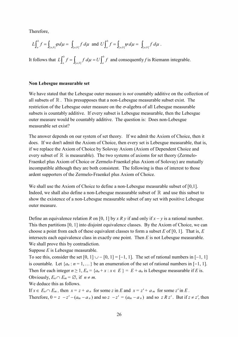
Non Lebesgue measurable set

We have stated that the Lebesgue outer measure is not countably additive on the collection of

all subsets of ℝ . This presupposes that a non-Lebesgue measurable subset exist. The

restriction of the Lebesgue outer measure on the -algebra of all Lebesgue measurable

subsets is countably additive. If every subset is Lebesgue measurable, then the Lebesgue

outer measure would be countably additive. The question is: Does non-Lebesgue

measurable set exist?

The answer depends on our system of set theory. If we admit the Axiom of Choice, then it

does. If we don't admit the Axiom of Choice, then every set is Lebesgue measurable, that is,

if we replace the Axiom of Choice by Solovay Axiom (Axiom of Dependent Choice and

every subset of ℝ is measurable). The two systems of axioms for set theory (Zermelo-

Fraenkel plus Axiom of Choice or Zermelo-Fraenkel plus Axiom of Solovay) are mutually

incompatible although they are both consistent. The following is thus of interest to those

ardent supporters of the Zermelo-Fraenkel plus Axiom of Choice.

We shall use the Axiom of Choice to define a non-Lebesgue measurable subset of [0,1].

Indeed, we shall also define a non-Lebesgue measurable subset of ℝ and use this subset to

show the existence of a non-Lebesgue measurable subset of any set with positive Lebesgue

outer measure.

Define an equivalence relation R on [0, 1] by x R y if and only if x y is a rational number.

This then partitions [0, 1] into disjoint equivalence classes. By the Axiom of Choice, we can

choose a point from each of these equivalent classes to form a subset E of [0, 1]. That is, E

intersects each equivalence class in exactly one point. Then E is not Lebesgue measurable.

We shall prove this by contradiction.

Suppose E is Lebesgue measurable.

To see this, consider the set [0, 1] [0, 1] = [1, 1]. The set of rational numbers in [1, 1]

is countable. Let {an : n = 1, } be an enumeration of the set of rational numbers in [1, 1].

Then for each integer n ≥ 1, En = {an + x : x E } = E + an is Lebesgue measurable if E is.

Obviously, En Em = if n m.

We deduce this as follows.

If x En Em , then x = z + a n for some z in E and x = z' + a m for some z' in E .

Therefore, 0 = z z' (am a n ) and so z z' = (am a n ) and so z R z' . But if z z', then

27

z and z ' would come from different equivalence classes and so z R z' cannot hold. Thus z z'

and so am = an, contradicting am a n .

For x in [0, 1] either x is in E or x R y for some y in E. Note that E E E a ,when

0a . If x R y for some y in E, then x y is a rational number in [1, 1]. Thus x y = aj

for some j. Hence, x = y + a j E + {aj } = Ej . We have thus shown that [0, 1] 1

ii

E

∪ .

Note that each En is a subset of [1, 2] and so 1

ii

E

∪ [1, 2] .

Now, for each i, ( Ei ) = ( E + ai ) =( E) as is translation invariant. Since each Ei is

measurable and 1i i

E

are pairwise disjoint, by the countable additivity of ,

1 1

lim [ 1, 2] 3i ini i

E E n E

∪ .

This is only possible if ( E) = 0. Therefore,1

0ii

E

∪ . But then we have, because [0, 1]

1

ii

E

∪ ,

1

1 [0,1] 0ii

E

∪ , which is absurd. Therefore, E is not Lebesgue

measurable.

Note that 1

1 * [0,1] * * [ 1, 2] 3ii

E

∪ .

If 1 1

* * lim *i ini i

E E n E

∪ , then it is only possible if (E) = 0 and so by

Proposition 16, E is Lebesgue measurable and we get a contradiction as before. This means

1 1

* *i ii i

E E

∪ , (E) > 0 and 1

1 * * [ 1, 2] 3ii

E

∪ . Hence, we can

conclude that the Lebesgue outer measure is not countably additive. It also follows that

there exists an integer n such that 1 1

* * *( )nn

i ii i

E E n E

∪ . This means that the

Lebesgue outer measure is also not finitely additive.

The following is a general way of getting a non-measurable set.

The device we would be using is the algebraic difference of two sets. This time we shall

obtain a non-measurable subset of ℝ . Define the same relation as before but now denote by

~ , on ℝ as follows. x ~ y if, and only if, x y is a rational number. Plainly, this is an

equivalence relation on ℝ . Denote the set of equivalence classes by /ℝ ∼ . Each equivalence

class has the form

:x r r ℚ .

28

Thus, the collection of rational numbers constitutes one equivalence class, 2 :r r ℚ is

another equivalence class and :r r ℚ is yet another. Obviously, each equivalence

class is countable and so since the set of real numbers ℝ is uncountable, the number of

distinct equivalence classes is uncountable. This is because if the number of equivalence

classes were countable then ℝ being the union of countable number of equivalence classes,

each of which is countable, would be countable and thus contradicts the fact that ℝ is

uncountable. By the Axiom of Choice, we can choose a point from each equivalence class to

form an uncountable set F. We claim that this set is non-measurable. This is because the set

of algebraic difference

F F = { x y: x, y F }

cannot contain an interval. Because any two distinct points of F must differ by an irrational

number and since F contains only one rational number, F F contains exactly one rational

number namely 0. If F F were to contain an interval, it would contain rational number

different from zero which is not possible. Hence by the following lemma, either F is not

Lebesgue measurable or *(F) = 0 and F is Lebesgue measurable.

Lemma 27. If E is a Lebesgue measurable subset of ℝ with positive measure, i.e., (E) >

0, then E E contains a non-trivial interval centred at the origin.

We shall prove this lemma later. Enumerate the set of rational numbers as {an : n = 1, }.

Now define Fn = {an + x : x F } = F + an . Then by the definition of F, we have

1n

n

F

ℝ ∪ . ---------------- (A)

Observe that by the definition of F, n mF F for n m so that 1

nn

F

ℝ ∪ is a countable

disjoint union.

If (F) = 0, then F is Lebesgue measurable by Proposition 16 and since is translation

invariant, (Fn) =(F + an ) (F) = 0. Thus, by the countable sub-additivity of the

Lebesgue outer measure, 1 1

*( ) * *( ) 0n nn n

F F

ℝ ∪ implying that *( ) 0 ℝ ,

which is not true. Hence *(F) 0. Therefore, by Lemma 27, F is not Lebesgue

measurable as F – F does not contain an interval.

We have thus produce two non-measurable subsets, one in [0, 1] and one in ℝ . We shall

make use of F to produce other non-measurable set.

Now for the proof of Lemma 27.

Proof of Lemma 27.

Suppose E is a Lebesgue measurable subset of ℝ with positive measure, i.e., (E) > 0 ,

Firstly, we take a special open set G containing E such that

29

(G) <(1 + )(E).

How can we obtain G? Recall that ( ) *( ) inf *( ) : ( )E E C E .

Now for any > 0, (1 + )(E)>(E). Therefore, by the definition of infimum, there exists a

countable cover of E, i.e., C(E), by open intervals such that

(1 + )(E) > () (E).

Let I

G I

∪ . Then G is an open set in ℝ and so is Lebesgue measurable. Since ℝ is

locally path connected, any open set of ℝ is also locally path connected and so G is locally

path connected. Hence, the path components are open sets and therefore, are open intervals.

As ℝ has a countable basis for its topology, these components are disjoint open cover for G

and can at most be countable. Thus, we conclude that G is a countable union of pairwise

disjoint open intervals. Let this collection of pairwise disjoint open intervals be denoted by

. ThenI I

G I I E

∪ ∪ . By the countable additivity of Lebesgue measure, ,

*( ) ( ) ( ) *( )I

I

G G I I

∪

* *( ) *( ) (1 ) ( )I

I

I I E

∪ ,

by the countable sub-additivity of *.

Thus, we have

( ) *( ) (1 ) ( )G E .

Let {In : n = 1, } be an enumeration of the open intervals in . Then 1

nI n

G I I

∪ ∪ . Let

En = E In. We have,

1 1 1

n n nn n n

E E G E I E I E

∪ ∪ ∪ .

Since In is Lebesgue measurable and E is Lebesgue measurable, En is Lebesgue measurable

for integer n ≥ 1. As ={In : n = 1, } is a countable collection of pairwise disjoint sets, {En

: n = 1, } is a countable collection of pairwise disjoint measurable subsets. Therefore, by

the countable additivity of the Lebesgue measure ,

1 1

( ) n nn n

E E E

∪ .

Note that 1 1

( ) n nn n

G I I

∪ . Since ( ) (1 ) ( )G E , we must have that for

some integer j ≥ 1,

( ) (1 ) ( )j jI E . ------------------- (1)

Let I = Ij and J = Ej . Then J = Ej = E Ij Ij = I.

Take = 1/3. Then by (1), (I) <(4/3)(J). That is,

(J) (3/4)(I) . ------------------------- (2)

30

We now claim that if J is translated by any number d with |d| < (1/2(I), the translated set

Jd has some points in common with J. If this is not the case, i.e., J Jd = , then since

J Jd I Id ,

2(J) = (J) + (Jd) = (J Jd ) (I Id ) (I) + |d| < (I) + (1/2(I) = (3/2)(I).

We would get (J) (3/4)I) contradicting (2).

Hence, J Jd ,

This means that for some y = x + d in Jd , where x is in J, y is also in J. Therefore, d = y x

is in J J. This is true for any d with |d| < (1/2(I) and so, the open interval

((1/2)(I), (1/2(I)) J J E E.

This completes the proof of lemma 27.

Theorem 28. For any subset A of ℝ with positive outer measure, i.e., (A) > 0, there is a

non-measurable subset B Proof.Suppose (A) > 0. Take Fn as defined before using the non-Lebesgue measurable

subset F of ℝ By (A), 1

nn

F

ℝ ∪ and so

1 1

n nn n

A A A F A F

ℝ ∪ ∪ .

Therefore,

1 1

* * *n nn n

A A F A F

∪ . ---------------- (1)

If A Fn is measurable, then since A Fn A Fn does not contain a non-trivial interval

(because Fn Fn dose not contain a non-trivial interval, a consequence of the fact that F F

dose not contain a non-trivial interval), by Lemma 27, (A Fn) = 0. Therefore, since (A)

> 0, A Fn cannot be measurable for all integer n. This is because if A Fn were

measurable for all integer n, then by (1), (A ) 0 contradicting (A) > 0. Hence, for

some integer j, A Fj is not Lebesgue measurable. Take B = A Fj .

This completes the proof of Theorem 28.

With this theorem proven, we conclude this modest introduction to the Lebesgue measure on

the real numbers ℝ .