Least-squares mixed finite elements for geometrically ... · Least-squares mixed finite elements...
140
Least-squares mixed finite elements for geometrically nonlinear solid mechanics Von der Fakult¨at f¨ ur Ingenieurwissenschaften, Abteilung Bauwissenschaften der Universit¨at Duisburg-Essen zur Erlangung des akademischen Grades Doktor-Ingenieur genehmigte Dissertation von Karl Steeger, M.Sc. Hauptreferent: Prof. Dr.-Ing. habil. J. Schr¨ oder Korreferenten: Prof. Dr. rer. nat. G. Starke Prof. Dr.-Ing. habil. A. D¨ uster Tag der Einreichung: 25. November 2016 Tag der m¨ undlichen Pr¨ ufung: 12. Mai 2017 Fakult¨atf¨ ur Ingenieurwissenschaften, Abteilung Bauwissenschaften der Universit¨at Duisburg-Essen Institut f¨ ur Mechanik Prof. Dr.-Ing. habil. J. Schr¨ oder
Transcript of Least-squares mixed finite elements for geometrically ... · Least-squares mixed finite elements...

Least-squares mixed finite elements for geometrically
nonlinear solid mechanics
Von der Fakultat fur Ingenieurwissenschaften,Abteilung Bauwissenschaftender Universitat Duisburg-Essen
zur Erlangung des akademischen Grades
Doktor-Ingenieur
genehmigte Dissertation
von
Karl Steeger, M.Sc.
Hauptreferent: Prof. Dr.-Ing. habil. J. SchroderKorreferenten: Prof. Dr. rer. nat. G. Starke
Prof. Dr.-Ing. habil. A. Duster
Tag der Einreichung: 25. November 2016Tag der mundlichen Prufung: 12. Mai 2017
Fakultat fur Ingenieurwissenschaften,Abteilung Bauwissenschaftender Universitat Duisburg-Essen
Institut fur MechanikProf. Dr.-Ing. habil. J. Schroder

Herausgeber:
Prof. Dr.-Ing. habil. J. Schroder
Organisation und Verwaltung:
Prof. Dr.-Ing. habil. J. SchroderInstitut fur MechanikFakultat fur IngenieurwissenschaftenAbteilung BauwissenschaftenUniversitat Duisburg-EssenUniversitatsstraße 1545141 EssenTel.: 0201 / 183 - 2682Fax.: 0201 / 183 - 2680
c© Karl SteegerInstitut fur MechanikAbteilung BauwissenschaftenFakultat fur IngenieurwissenschaftenUniversitat Duisburg-EssenUniversitatsstraße 1545141 Essen
Alle Rechte, insbesondere das der Ubersetzung in fremde Sprachen, vorbehalten. OhneGenehmigung des Autors ist es nicht gestattet, dieses Heft ganz oder teilweise auffotomechanischem Wege (Fotokopie, Mikrokopie), elektronischem oder sonstigen Wegenzu vervielfaltigen.
ISBN-10 3-9818074-1-3ISBN-13 978-3-9818074-1-7EAN 9783981807417

Fur Kristina und Gabriel


5
Vorwort
Die vorliegende Arbeit entstand wahrend meiner Tatigkeit als wissenschaftlicher Mitar-beiter am Institut fur Mechanik (Abteilung Bauwissenschaften, Fakultat fur Ingenieur-wissenschaften) an der Universitat Duisburg-Essen unter anderem im Rahmen des durchdie Deutsche Forschungsgemeinschaft (DFG) finanzierten Projektes SCHR 570/14-1,STA 402/11-1. An dieser Stelle mochte ich der DFG fur die finanzielle Unterstutzungdanken und meinen personlichen Dank an einige Menschen aussprechen, die ihren jeweili-gen Anteil zum Gelingen dieser Arbeit beigetragen haben.Zuallererst mochte ich meinem geschatzten Doktorvater Professor Jorg Schroder aufrichtigdanken, der mir die Moglichkeit gab unter seiner Leitung zu promovieren. Ihm gilt derDank fur die Forderung wahrend der gesamten Promotionszeit. Seine besondere Artund Weise der Motivation wahrend der gesamten Zeit und sein Enthusiasmus fur dieMechanik waren fur mich stets eine Quelle der Inspiration. Besonders danken mochteich auch Professor Gerhard Starke, sowohl fur die Ubernahme des Zweitgutachtens alsauch fur die erfolgreiche Zusammenarbeit im Rahmen des gemeinsamen DFG Projektesund daruber hinaus. Bei vielen Diskussionen habe ich sein weitreichendes Wissen in derMathematik zu schatzen gelernt. Weiterhin gilt mein Dank auch Professor AlexanderDuster fur sein Interesse an der Arbeit und die Ubernahme des externen Gutachtens. Ichdanke Professor Joachim Bluhm, der sich jederzeit gerne fur fachliche AngelegenheitenZeit nahm. Sein Wissen und seine Erfahrung fuhrten stets zu guten Ratschlagen. Einherzliches Dankeschon auch an meine Wegbegleiter Bernhard Eidel, Marc-Andre Keipund Oliver Rheinbach, deren Kompetenzen und ihre Bereitschaft diese zu teilen mir stetseine große Hilfe waren. Dominik Brands gilt mein Dank fur jede Art von Unterstutzunghinsichtlich der Administration, eingeschlossen der Pflege meines Rechners. Ebenfallsmochte ich Benjamin Muller und Fleurianne Bertrand fur die Zusammenarbeit und denmathematischen Austausch danken.Ein besonderer Dank gilt meinen studentischen Hilfskraften Robert Depenbrock,Maximilian Igelbuscher, Sascha Maassen, Dominik Ohlmann, Yasemin Ozmen und NilsViebahn fur die intensive (und teilweise noch andauernde) Zusammenarbeit. Sie schenk-ten mir ihr Vertrauen, gaben mir die Moglichkeit sie zu fordern und ihre Abschlussarbeitenzu betreuen. Es erfullt mich mit Stolz zu sehen, wozu sie es bereits heute schon gebrachthaben. Daruber hinaus mochte ich Alexander Schwarz danken, der mich bereits wahrendmeines Bachelorstudium gefordert hat. Ich durfte an die wissenschaftlichen Erkenntnisseseiner Promotion anknupfen und er war jederzeit bereit, sein breites Wissen mit mir zuteilen. Die vielen Diskussionen uber finite Elemente fuhrten oft zu wesentlichen Erkennt-nisgewinnen.Aufs Herzlichste mochte ich meinen derzeitigen und ehemaligen Kolleginnen und Kolle-gen am Institut danken, zu denen Solveigh Averweg, Daniel Balzani, Julia Bergmann,Moritz Bloßfeld, Sarah Brinkhues, Vera Ebbing, Simon Fausten, Markus von Hoegen,Veronika Jorisch, Marc-Andre Keip, Simon Kugai, Matthias Labusch, Veronica Lemke,Petra Lindner-Roulle, Simon Maike, Rainer Niekamp, Carina Nisters, Mangesh Pise,Sabine Ressel, Lisa Scheunemann, Thomas Schmidt, Serdar Serdas, Steffen Specht undHuy Ngoc Thai gehoren.Meinen Eltern, meinen Schwiegereltern und meiner gesamten Familie mochte ich dankenfur die immerwahrende Unterstutzung. Abschließend danke ich meiner Frau Kristina, dieden langen Weg zur Promotion mit mir gegangen ist. Ihre Geduld, ihr Verstandnis undihre Fursorge waren mir stets eine große Hilfe.
Essen, im Juni 2017 Karl Steeger


7
Abstract
The computation of reliable results using finite elements is a major engineering goal.Under the assumption of a linear elastic theory many stable and reliable (standard andmixed) finite elements have been developed. Unfortunately, in the geometrically non-linear regime, e.g. applying these elements in the field of incompressible, hyperelasticmaterials, problems can occur. A possible approach to circumvent these issues might bethe least-squares mixed finite element method. Therefore, in this thesis, a mixed least-squares formulation for hyperelastic materials in the field of solid mechanics is provided,investigated and valuated. To create a theoretical basis the continuum mechanical back-ground is outlined, the necessary physical quantities are introduced and the constructionof suitable interpolation functions for the interpolation in W 1,p(B) (using standard inter-polation polynomials) and W q(div,B) (using vector-valued Raviart-Thomas interpolationfunctions) are derived. Furthermore, the general procedure for the construction of a least-squares functional is described and applied for hyperelastic material laws based on a freeenergy function. Basis for the proposed least-squares element formulation is a div-gradfirst-order system consisting of the equilibrium condition, the constitutive equation anda stress symmetry condition, all written in a residual form. The solution variables (dis-placements and stresses) are, dependent on the element type, interpolated using differentapproximation spaces. The resulting elements are named as PmPk and RTmPk. Here m(stresses) and k (displacements) denote the polynomial order of the particular interpola-tion function. The performance of the provided elements is investigated and compared tostandard and mixed Galerkin elements by extensive numerical studies with respect to e.g.bending dominated problems, incompressibility, stability issues, convergence of the fieldquantities and adaptivity. Furthermore, the crucial influence of weighting is discussed.Finally, the results are evaluated and the used elements are assessed.
Zusammenfassung
Ein Hauptziel im Bereich des Ingenieurwesens ist die Berechnung vertrauenswurdigerErgebnisse mit Hilfe der Methode der finiten Elemente. Unter Annahme einer linearelastischen Theorie wurden hierzu bereits viele stabile und zuverlassige standard undgemischte finite Elemente entwickelt. Es hat sich jedoch herausgestellt, dass bei eini-gen dieser Elemente, unter anderem angewandt auf inkompressible, hyperelastische Ma-terialien, Probleme auftreten. Ein moglicher Ansatz um diese Probleme zu umgehenist moglicherweise die gemischte least-squares finite Elemente Methode. Daher wird inRahmen dieser Arbeit eine gemischte least-squares Formulierung fur hyperelastische Ma-terialien vorgestellt, untersucht und bewertet. Um eine theoretische Basis zu schaffenwird zuerst ein kontinuumsmechanischer Rahmen geschaffen, die notigen physikalischenGroßen werden eingefuhrt und die Konstruktion geeigneter Interpolationsfunktionen zurInterpolation in W 1,p(B) (mit standard Interpolationspolynomen) und W q(div,B) (mitvektorwertigen Raviart-Thomas Interpolationsfunktionen) werden hergeleitet. Im Fol-genden wird das allgemeine Vorgehen zur Konstruktion eines least-squares Funktionalsbeschrieben und angewandt auf hyperelastische Materialien in der Festkorpermechanikbasierend auf freien Energiefunktionen. Die Basis fur die least-squares Formulierungstellt ein div-grad System erster Ordnung dar, bestehend aus der Gleichgewichtsbedin-gung, einem Materialgesetz und einer zusatzlichen Bedingung fur die Einhaltung einerSpannungssymmetrie. Die Gleichungen liegen hierbei in einer residualen Form vor. Die

8
Losungsvariablen sind, im Rahmen dieser Arbeit, die Verschiebungen und die Spannungenwelche, abhangig vom Elementtyp, mit unterschiedlichen Interpolationsfunktionen inter-poliert werden. Die resultierenden Elemente werden bezeichnet als PmPk und RTmPk,wobei m und k die jeweilige Interpolationsordnung zur Approximation der Spannungen(m) und der Verschiebungen (k) angeben. Die Performanz der entwickelten Elemente wirdim Folgenden mit extensiven numerischen Studien untersucht, welche sich unter anderemmit biegedominierten Problemen, Inkompressibilitat, Untersuchung von Stabilitatspunk-ten und der allgemeinen Konvergenz der Losungsvariablen beschaftigen. Zur Bewertungder Ergebnisse werden diese mit Losungen verglichen, welche durch standard und gemis-chte Galerkin Elemente berechnet wurden. Daruber hinaus wird der starke Einfluss derWichtungsfaktoren auf die Qualitat der Losungen diskutiert. Abschließend werden dieErgebnisse ausgewertet und die entwickelten Elemente bewertet.

Table of Contents I
Contents
1 Introduction 1
1.1 Galerkin and mixed Galerkin finite elements . . . . . . . . . . . . . . . . . 1
1.2 Least-squares mixed finite elements . . . . . . . . . . . . . . . . . . . . . . 2
1.3 Outline . . . . . . . . . . . . . . . . . . . . . . . . . . . . . . . . . . . . . . 4
2 Continuum mechanical background 7
2.1 Kinematics and deformation measures . . . . . . . . . . . . . . . . . . . . 7
2.2 Stress quantities . . . . . . . . . . . . . . . . . . . . . . . . . . . . . . . . . 10
2.3 Hyperelastic materials . . . . . . . . . . . . . . . . . . . . . . . . . . . . . 11
2.3.1 Neo-Hookean . . . . . . . . . . . . . . . . . . . . . . . . . . . . . . 12
2.3.2 Mooney-Rivlin . . . . . . . . . . . . . . . . . . . . . . . . . . . . . 13
2.3.3 Transverse isotropic hyperelasticity . . . . . . . . . . . . . . . . . . 13
3 Interpolation 15
3.1 Interpolation spaces . . . . . . . . . . . . . . . . . . . . . . . . . . . . . . . 15
3.2 Discretization of W 1,p(B) . . . . . . . . . . . . . . . . . . . . . . . . . . . . 15
3.3 Discretization of W q(div,B) . . . . . . . . . . . . . . . . . . . . . . . . . . 16
3.3.1 Basis functions for order m = 1. . . . . . . . . . . . . . . . . . . . . 20
3.4 Alternative discretization of W q(div,B) . . . . . . . . . . . . . . . . . . . . 22
4 The least-squares mixed finite element method 25
4.1 Construction of least-squares functionals . . . . . . . . . . . . . . . . . . . 25
4.2 General setup for the hyperelastic least-squares formulation . . . . . . . . . 26
4.3 Interpolation of field quantities . . . . . . . . . . . . . . . . . . . . . . . . 28
4.4 Introductory example in 1D . . . . . . . . . . . . . . . . . . . . . . . . . . 29
4.5 Different least-squares element types under investigation . . . . . . . . . . 36
4.5.1 Position of the interpolation sites and number of element degrees offreedom . . . . . . . . . . . . . . . . . . . . . . . . . . . . . . . . . 37
4.5.2 Resulting interpolation matrices . . . . . . . . . . . . . . . . . . . . 37
4.6. Boundary conditions . . . . . . . . . . . . . . . . . . . . . . . . . . . . . . . 41
4.6.1. Example for the application of boundary conditions . . . . . . . . . . 42
4.7. Remarks on the implementation . . . . . . . . . . . . . . . . . . . . . . . . 43
4.7.1. General remarks . . . . . . . . . . . . . . . . . . . . . . . . . . . . . 43
4.7.2. General element setup in AceGen . . . . . . . . . . . . . . . . . . . . 44

II CONTENTS
5 Investigation of the performance of different element types under consid-eration of different physical quantities and influence of scalar weighting 47
5.1 Cantilever beam, performance study . . . . . . . . . . . . . . . . . . . . . 48
5.2 Cantilever beam, influence of weighting . . . . . . . . . . . . . . . . . . . . 51
5.3 Cook’s Membrane, stress distribution and reaction forces . . . . . . . . . . 53
5.4 Quartered plate, convergence of stresses . . . . . . . . . . . . . . . . . . . . 58
5.5 Compression test, compliance with volume conservation . . . . . . . . . . . 61
5.6 3D plate, displacement convergence and stress distribution . . . . . . . . . 62
5.7 Cantilever beam, influence of transverse isotropy . . . . . . . . . . . . . . . 64
6 Locking phenomena 67
6.1 Cantilever beam, investigation of locking . . . . . . . . . . . . . . . . . . . 67
7 Adaptive mesh refinement 73
7.1 Marking strategies . . . . . . . . . . . . . . . . . . . . . . . . . . . . . . . 74
7.1.1 Element percent marking strategy (arE) . . . . . . . . . . . . . . . 75
7.1.2 Error percent marking strategy (arD) . . . . . . . . . . . . . . . . . 75
7.2 Refinement strategies . . . . . . . . . . . . . . . . . . . . . . . . . . . . . . 75
7.3 Plate with a hole, investigation of adaptive mesh refinenemt . . . . . . . . 76
8 Bifurcation analysis 83
8.1 Euler buckling cases . . . . . . . . . . . . . . . . . . . . . . . . . . . . . . 84
8.2 Example 2: Stability points, compare Auricchio et al. [2010] and Auricchioet al. [2013] . . . . . . . . . . . . . . . . . . . . . . . . . . . . . . . . . . . 86
8.2.1 Stability points, problem 2 in Auricchio et al. [2010] . . . . . . . . . 86
8.2.2 Stability points, problem 1 in Auricchio et al. [2013] . . . . . . . . . 88
9 Summary, conclusion and outlook 89
A Appendix 93
A.1 Basis functions for order m = 2 . . . . . . . . . . . . . . . . . . . . . . . . 93
A.2 Basis functions for order m = 3 . . . . . . . . . . . . . . . . . . . . . . . . 96
A.3 Alternative basis functions for order m = 1 . . . . . . . . . . . . . . . . . . 101
A.4 Alternative basis functions for order m = 2 . . . . . . . . . . . . . . . . . . 101
A.5 Alternative basis functions for order m = 3 . . . . . . . . . . . . . . . . . . 102
A.6 Further courses of the reaction forces for the Cook’s Membrane example . . 105
A.7 Shear stress distribution for the example of the quartered plate. . . . . . . 105

Introduction 1
1 Introduction
In this day and age the solution of physical problems on arbitrary domains using numericalsimulation methods is widely spread and established in almost all engineering areas. Thisbecomes possible due to the raising computer power which growth followed, at least upto the last years, Moore’s law, see Moore [1965]. In the field of solid mechanics the finiteelement method (FEM) is therefore an almost indispensable integral part of modelingand simulation in engineering applications. The origin of the method can be found in the1950’s inter alia by Argyris and Kelsey [1954], Argyris [1955] and Turner et al. [1956]. Theterminology “finite element” has then been introduced by Clough [1960]. In the followingdecades the method has been extendend and examined further. An overview over thepublications with respect to the finite element method is provided, for instance, in Noor[1991] or more recently in the historical overview over various milestones of Stein [2012].Furthermore, for a comprehensive collection of todays computational methods the readeris referred to the book series of Stein et al. [2004].
1.1 Galerkin and mixed Galerkin finite elements
The underlying variational principle for the solution of the given differential equations ismostly the so-called Galerkin method (Standard Galerkin method), which origin is givenin Galerkin [1915]. This method is, in the field of solid mechanics, often restricted on thedisplacement as field quantitiy. Unfortunately, certain problems limit the applicabilityof the standard method. That means, that for example incompressible materials couldlead to not well-posed formulations. In the case of incompressible or nearly incompressiblematerials volumetric locking can be observed, resulting in a lower convergence behavior oreven a pathological approximation of the stresses, see e.g. Babuska and Suri [1992]. Fur-thermore, in the field of the standard displacement based FEM the stresses are generallycomputed as the derivatives of a C0 continuous function. This leads to a stress field whichcould be discontinuous at element interfaces. In addition to that, for bending-dominatedproblems, standard approaches could cause shear locking. In this context ”standard”means the classical linear respectively quadratic Galerkin elements. Possible approachesto overcome this problems is to use high-order elements, compare e.g. Duster et al. [2003],Heisserer et al. [2008] and Netz et al. [2013] or to use mixed finite elements.
The basis for these mixed formulations are here mostly variational formulations ofHellinger-Reissner or Hu-Washizu type. To ensure the stability of the resulting sad-dlepoint structure, methods of this type have to fulfill the so-called LBB-condition(Ladyzhenskaya-Babuska-Brezzi-Bedingung), based on Ladyzhenskaya [1969], Babuska[1973] and Brezzi [1974]. An overview over the analysis can be found e.g. in Bathe [1995],Bathe [2001] and Ern and Guermond [2013]. This condition demands to balance thechosen interpolation orders for the different field quantities. The first hybrid stress finiteelement, based on the minimum of a complementary energy has been developed by Pian[1964]. Drawbacks of this approach concerning invariance requirements has been elimi-nated by Pian and Sumihara [1984]. The basis was a Hellinger-Reissner functional, wherestresses and displacements were used as basic field variables. Using a non-symmetric ap-proximation of the stress field, Klaas et al. [1995] developed a formulation based on anextended dual Hellinger-Reissner functional with two additional unknown fields leadingto optimal convergence rates for the displacements and stresses which are approximated

2 Introduction
by Brezzi-Douglas-Marini (BDM) elements, see Brezzi et al. [1985]. Further studies con-cerning elasto-plasticity problems can be found in Schroder et al. [1997]. On the basis ofa Hu-Washizu functional a further approach, the so-called F -method, was developed bySimo et al. [1984]. This formulation makes use of the multiplicative split of the deforma-tion gradient into volumetric and isochoric parts. In particular for lower order elementscertain versions of this have been successfully applied, see de Souza Neto et al. [1996;2005]. Beyond that, ideas dealt with non-locally averaged nodal stress and deformationquantities. For further approaches, where averages of the pressure or deformation quan-tities are taken into account over domains that are associated to nodes, edges and faces,see e.g. Dohrmann et al. [2000], Gee et al. [2009], and Liu and Nguyen-Thoi [2010]. Amajor drawback is that such elements can not be implemented with an acceptable effortin standard commercial finite element software, which is due to the nonlocal averagingoperator. Furthermore, the method of incompatible modes, see Wilson et al. [1973] andTaylor et al. [1976], was the starting point for the class of mixed enhanced strain elementformulations. Based on the three-field Hu-Washizu functional the Enhanced-Assumed-Strains (EAS) approach has been provided respectively investigated by Simo and Rifai[1990], Simo and Armero [1992] Simo et al. [1993], Reddy and Simo [1995], and Freis-chlager and Schweizerhof [1996]. Unfortunately, the enhanced elements may encountermesh-instabilities, such as hourglassing, see Wriggers and Reese [1996]. In this context,reduced integration as well as stabilization techniques can be found in e.g., Bischoff et al.[1999], Reese et al. [1999] and Reese and Wriggers [2000]. A recent publication giving anextensive overview over mixed finite element methods is given by Boffi et al. [2013].
1.2 Least-squares mixed finite elements
A further finite element approach, which increasingly gains attention in the last decades,is the least-squares method. Initially, the least-squares method is the standard approachfor regression analysis where it is used to compute, for an arbitrary number of datapoints,a curve which fulfills the given points in a least-squares sense.
The least-squares finite element method (LSFEM) is characterized by several advantages.The LSFEM replaces, for instance, a constrained minimization problem (with saddlepointstructure) by a least-squares formulation without constraints. Thus, it is not restricted bythe latter mentioned LBB-condition and it is possible to combine (more or less arbitrary)polynomial orders for the interpolation of the unknowns without losing stability proper-ties. Furthermore, the resulting system matrices are always positive definite which couldbe advantageous for the applied solver. In addition to that the least-squares functionalcan be set up using freely selectable field variables and governing equations. A furtheradvantage of the method is that the functional is usable as an inherent a posteriori errorindicator, compare e.g. Cai and Starke [2004] and Bochev and Gunzburger [2009]. Thatmeans, that for an adaptive mesh refinement strategy no additional costs has to be in-vested in the error estimation. Unfortunately, the method, as far it has been investigateduntil today, contains also several disadvantages. Here the weak performance of low orderelements has to be mentioned, compare e.g. Pontaza [2003], Pontaza and Reddy [2003]and Schwarz et al. [2010]. Furthermore, the used (physical) residuals respectively theirweighting have a crucial impact on the accuracy of the solution and have to be balancedsuitably. First applications of the least-squares method in the field of finite elements re-spectively their mathematical analysis can be found e.g. in Lynn and Arya [1973; 1974],

Introduction 3
Zienkiewicz et al. [1974], Jespersen [1977] and Fix et al. [1979]. An overview over theleast-squares method and its first applications in the field of finite elements is given inEason [1976]. Furthermore, in this publication inter alia the advantages of the methodare already discussed. In the following decade the number of publications concernig thistopics reduces (e.g. Aziz et al. [1985]). This is eventually due to weak approximationquality for lower order elements which where mainly used at that time. The beginningof the 1990’s brought a boom for the method, which was mainly restricted on the fieldof fluid mechanics, compare e.g. Jiang and Chang [1990], Chang and Jiang [1990], Jiang[1992], Tang and Tsang [1993], Cai et al. [1994], Bochev and Gunzburger [1994; 1995],Cai et al. [1995], Chang et al. [1995], Bell and Surana [1994], Bochev [1994; 1999], Berndtet al. [1997], Bochev et al. [1998], Bochev et al. [1999], Ding and Tsang [2001; 2003],Pontaza and Reddy [2003], Kayser-Herold and Matthies [2003] and Kayser-Herold andMatthies [2007]. Here, the used first-order systems interpolate different combinationsas, for instance, the flow velocity, the pressure, the stresses or the vorticity field. Theapproximation of these unknown quantities was mainly restricted on the Sobolev spaceH1(B). For an overview over the developments of the least-squares method in the field offluid mechanics the reader is referred to Jiang [1998], Bochev and Gunzburger [2009] andKayser-Herold and Matthies [2005] and the references therein.
In the field of solid mechanics the number of publications considering the least-squaresmethod is significantly smaller. First formulations can be found e.g. in Cai et al. [1995],where a formulation for linear elastic problems has been provided. Therefore, the authorsused as a basis a div-curl-grad system of first-order with the unknown fields velocity, vor-ticity and pressure (VVP). Further investigations of this working group, also in the fieldof linear elastic problems, are inter alia Cai et al. [1997; 1998; 2000a;b] and Kim et al.[2000]. In this publications the displacement and the displacement gradient are used asfield quantities and are interpolated in H1(B). In the works of Cai and Starke [2004] andCai et al. [2005] the authors used the displacement and the stresses as unknown fields.The approximation of the quantities has been executed in H1(B) via standard polynomialinterpolation for the displacement field and, for the stress field, vector-valued interpola-tion functions of Raviart-Thomas type, see Raviart and Thomas [1977], in H(div,B).This choice of interpolation spaces has been continued for instance in Schwarz [2009] andSchwarz et al. [2010]. In the latter mentioned publications also the suitability of the func-tional as an error indicator, the fulfillment of the stress symmetry as well as the behaviorof the formulations considering (nearly) incompressible materials is discussed. Further-more, a main benefit of the formulation in Schwarz et al. [2010] is the good performanceof the developed low order element. This is due to a modification of the first variation ofthe functional and the resulting improvement of the momentum balance. An extensionon transversely isotropic elasticity can be found in Schwarz and Schroder [2007] and inSchwarz et al. [2014] a least-squares formulation with an additional (redundant) residualhas been used. In Bertrand et al. [2014] the application of the first-order system least-squares method on curved boundaries is provided. In the field of material nonlinearities,in detail elasto-plasticity, Kwon et al. [2005] and Starke [2007] published results. A mainissue in this context has been the non-smoothness of the constitutive relation in the caseof plastic deformations and the resulting problems using standard nonlinear solver. Toovercome this, Starke [2009] used a non-smooth Newton method which results in suitableconvergence rates. In the work of Schwarz et al. [2009b] this issue is circumvented by amodified approach and in Schwarz et al. [2009a] the authors used a viscoplastic formu-

4 Introduction
lation. In Steeger et al. [2015] the authors investigate a displacement-stress formulationwhere they consider the performance using an interpolation of the stresses in H(div,B)compared to an interpolation of the stresses in H1(B). In the publications of Jiang andWu [2002] and Jiang [2002] two different formulations are taken under consideration. InJiang and Wu [2002] (part 1), beside the displacement and the stresses, the rotation withrespect to the plane normal is used as a basis for the formulation. The second part (Jiang[2002]) considers a formulation for the computation of bending problems considering thinplates. Therefore, the author used a first-order system which depends on four differentquantities and shows optimal convergence rates in the provided examples.
First investigations in the field of geometrically nonlinear problems in the field of solidmechanics are e.g. Westphal [2004] and Manteuffel et al. [2006] where a constitutiverelation of St.Venant-Kirchhoff type has been considered. As of late also least-squaresformulations for hyperelastic problems has been developed, see e.g. Schwarz et al. [2012],Starke et al. [2012], Muller et al. [2014], Muller [2015] and Muller and Starke [2016].In Schroder et al. [2016] several least-squares formulations for isotropic and anisotropicelasticity at small and large strains are given. In Kadapa et al. [2015] a formulation usingthe displacements and the pressure as field quantities, interpolated by NURBS (non-uniform rational B-splines), has been provided. Here, fluid mechanical problems as wellas problems in the field of solid mechanics (hyperelasticity) are taken under consideration.
1.3 Outline
This work is organized as follows: After a brief introduction of the used physical quan-tities and the essential continuum mechanical relations several hyperelastic free-energyfunctions are given in Section 2. The used interpolation spaces W 1,p(B) and W q(div,B)are introduced and the derivation of suitable functions for the approximation in thesespaces are shown for different interpolation orders in Section 3. Here, especially theconstruction of vector-valued Raviart-Thomas functions is discussed in detail. Further-more, an alternative way for the development of such functions is described. Section4 provides the general rule for construction of a least-squares functional followed by thederivation of a least-squares mixed finite element formulation for hyperelastic free energyfunctions. After that, for a deeper understanding of the method, the application of theLSFEM on an one-dimensional example is considered. Here, starting from the governingdifferential equation all steps up to the solution of a simple boundary value problem arediscussed in detail. As the least-squares mixed finite element method is not restricted tothe LBB-condition, in the following different element types are provided and the resultingnumber of degree of freedom per element are given. Furthermore, some remarks are givenon the application of boundary conditions for the different field quantities. Therefore,the difference between the application of boundary conditions for the two element types(RTmPk and PmPk) is shown by a simple example. Finally, in this Section some remarkson the implementation are given. Therefore, individual parts of the codes are shown togive a brief overview over the implementations in AceGen. In Section 5 several numeri-cal benchmark problems are taken under consideration. First the example of a cantileverbeam shows the performance of the formulation considering different interpolation ordersas well as different element types (RTmPk and PmPk). In the following the influence ofthe scalar weighting factor ω3 on the performance considering this bending dominatedproblem is shown. The next boundary value problem under consideration is the Cook’s

Introduction 5
Membrane problem. Here, the distribution of the stresses of a least-squares finite ele-ment is compared to a standard and a mixed Galerkin element. Furthermore, using thisexample, the ability of the method to compute support reactions is investigated. Thefollowing example of a quartered plate aims to show the performance of the differentelement types with respect to the computation of stresses for a boundary value problemconsisting of different materials. In addition to that the benchmark of the compressiontest is provided, compare Reese and Wriggers [2000]. As a three-dimensional examplethe benchmark problem of a clamped plate is taken under consideration. Finally, theperformance of the least-squares formulation under assumption of a transversely isotropicmaterial is investigated.
The locking phenomena could be an important issue for finite element formulations.Therefore, in Section 6, the influence of a raise of the Lame paramter λ (respectively thePoisson’s ration ν → 0.5) which is the so-called volumetric locking or Poisson’s locking, isinvestigated. Therefore, the term “locking” is defined and the influence to the providedleast-squares mixed finite element is tested by means of a numerical example.
As the least-squares functional is usable as an error indicator, the application of adaptivemesh refinement is a cost-effective method to improve the performance of the elements.In Section 7, after a brief introduction into the theory of adaptive mesh refinement, twodifferent marking strategies are presented. In the following, the benchmark problem of aplate with a hole is considered. There, a regular mesh refinement as well as an adaptivemesh refinement is used for the computation of the result. For comparison the resultantconvergence rates are taken under consideration.
Due to stability issues for several mixed finite element formulations presented in Auricchioet al. [2010] and Auricchio et al. [2013], in Section 8 the ability of the provided elementformulation for the computation of stability points for several numerical examples areshown. As the least-squares method, due to its structure, cannot produce negative eigen-values, a different definition for the detection of the critical loads is neccesary. Therefore,the definition of Muller et al. [2014] is used and the results are compared to a standardGalerkin element.
Finally, in Section 9 the discussed topics are summarized and a conclusion is drawnconcerning the obtained findings. Furthermore, at the end of this work, an outlook isgiven pointing out further issues, which could be discussed in future work.


Continuum mechanical background 7
2 Continuum mechanical background
In the field of computational mechanics mostly materials are assumed to be a continuum.The real material structure is in general inhomogeneous at least on an atomistic level.But even on higher scales (as e.g. on the microscopic level) the material properties arenot continuous (as e.g. different grain size distributions). However, the simplificationto a continuous material and the disregard of the microstrucure leads, in general, tosufficiently accurate results for the prediction of the physical behavior. Therefore, certainfield quantities as e.g. the displacements or the stresses replace the complex behaviorof the real physical body. Due to the definition as a continuum the complete materialbehavior can be described in an inner material point of the domain, which contains allphysical state quantities. The assumption of a physical body as continuous mediumis the basis for the so-called continuum mechanics, which fundamentals can be found inTruesdell and Toupin [1960], Truesdell and Noll [1965] and Eringen [1967]. Further generalcontinuum mechanical literature is given e.g. by Marsden and Hughes [1994], Stein andBarthold [1996], Silhavy [1997], Holzapfel [2000], Truesdell and Noll [2004] and Parisch[2013]. The present work is restricted to solid bodies which are assumed to be a continuumand purely elastic. First, the necessary kinematical quantities and deformation measureswill be introduced. Furthermore, several stress quantities will be presented. In the nextsubsection different hyperelastic free energy functions will be given. In the framework ofthis work the derivations of the balance principles and the entropy inequality are omittedand the interested reader is referred to standard textbooks as e.g. Holzapfel [2000] orWriggers [2001].
2.1 Kinematics and deformation measures
For the description of an arbitrary movement of a body in space its kinematics has to bedefined. Therefore, a continuous body in the so-called “reference configuration” B0 ⊂ R3,with the Euclidian space R3, parametrized in X, with the boundary ∂B0 is defined. Eachmaterial point (particle) of the body B0 (the location) can be described by its positionvectorX. If this body undergoes movements in terms of deformations, translations and/orrotations the body changes its position to new ones at time t ∈ R+, where the position ofeach particle of the body can be described by a position vector xt. These configurationsof the body Bt ⊂ R3 with the boundary ∂Bt are called “current configurations”. Themotion (mapping) between reference and current configuration is then given by
xt(X, t) = ϕ(X, t) : B0 → Bt , (1)
which maps every point X ∈ B0 to a point x ∈ Bt. In the following, for simplification,further derivations are restricted on one current placement at a fixed time t and neglect,for quantities referring to the current placement, the subscript t leading to
x(X) = ϕ(X) : B0 → B. (2)
The arising displacement is given by u(x) = x−X. On both bodies an infinitesimal line,vectorial area and volume element dX, dA and dV (on B0) respectively dx, da and dv(on Bt) can be defined, see also Figure 1.

8 Continuum mechanical background
BtB0
x = ϕt(X)
Cof F
F
detF
dx
dVdv
dX
dadA
Figure 1: Mappings of the infinitesimal line, area and volume elements, F : dX 7→dx,Cof F : dA 7→ da and detF : dV 7→ dv.
The current position vector x is given as
x = X + u . (3)
With this in hand, the deformation gradient F , a fundamental kinematical quantitiy de-fined as the gradient of the mapping ϕ(X) in Equation (2) with respect to the coordinatesX, is given as
F =∂ϕ
∂X=
∂x
∂X= I+∇u . (4)
Here, ∇ denotes the gradient with respect to the reference configuration. The deformationgradient can be used for the mapping between the reference and the current configuration.The mapping between an infinitesimal line element in the reference configuration dX andan infinitesimal line element dx in the current configuration is given by
dx = F dX . (5)
With two independent infinitesimal line elements denoted by
dx = F dX and dy = F dY , (6)
an infinitesimal vectorial area element da can be defined given by the cross product
da = dx× dy . (7)
For the mapping of the area element from the reference to the current configuration with
dA = N dA and da = n da (8)
and Equation (6) and Equation (7)
da = (F dX)× (F dY ) = Cof[F ] ( dX × dY ) = Cof[F ] dA (9)

Continuum mechanical background 9
is obtained, with N and n as the unit normal vectors of the associated area elements.Here, Cof F denotes the cofactor given as
Cof F = det[F ]F −T ,
under the assumption of an invertible deformation gradient
F−1 =∂X
∂x. (10)
An infinitesimal volume element in the reference configuration dV = dA · dZ can bemapped to an infinitesimal volume element in the current configuration dv = da · dzusing the determinant of the deformation gradient
dv = J dV ,
where J denotes the determinant of the deformation gradient J = detF . All describedmappings are depicted in Figure 1.
Since the deformation gradient F includes rigid body rotations and can be split in a leftand right stretch tensor (V , U) and an orthogonal rotation tensor R it can be written as
F = RU = VR . (11)
Further deformation measures, which are free from rigid body rotations and just accountfor the pure stretch part of the defomation are the nonlinear deformation measures
C = F TF = U 2 and b = FF T = V 2. (12)
C is denoted as right Cauchy-Green deformation tensor and b as left Cauchy-Greendeformation tensor (respectively Finger tensor). Another deformation measure is theGreen-Lagrange strain tensor E, given as
E =1
2(C − I) =
1
2(∇u+ (∇u)T + (∇u)T∇u). (13)
For the description of hyperelastic material behavior a so-called Helmholtz free energyfunction ψ(F ) respectively the appropriate strain energy density W (F ) = ρ0ψ(F ) de-fined per unit volume with the reference density ρ0 is used. As it is important, that thedescription of the material behavior is invariant with respect to superimposed rigid bodyrotations onto the spatial placement, the principle of material frame indifference (principleof objectivity) has to be satisfied. Using the right Cauchy-Green tensor C as deformationmeasure in the free energy function, the principle is fulfilled, compare e.g. Truesdell andNoll [1965]. Therefore the principle of material symmetry has to be fulfilled, compare alsoSchroder et al. [2016]. Hence, the hyperelastic free energy is written in terms of the prin-cipal invariants (respectively the main invariants) of the right Cauchy-Green deformationtensor given as
I1 = trC, I2 = tr[CofC] = tr[det[C]C−1], I3 = detC = J2 (14)

10 Continuum mechanical background
respectivelyJ1 = tr C, J2 = tr[C2], J3 = tr[C3]. (15)
Both types of invariants can be transferred into each other. In the following also trans-verse isotropic hyperelastic materials are taken under consideration. Therefore, the mixedinvariants
I4 = tr[CM ] and I5 = tr[Cof[C]M ] , (16)
have to be introduced. Here M denotes a structural tensor given by
M = a⊗ a , (17)
with a denoting the preferred direction in the reference configuration and |a| = 1. Fordetailed discussions about the construction of hyperelastic free energy functions, coerciv-ity, convecxity and further informations about the satisfaction of the latter mentionedprinciples the reader is referred to e.g. Schroder and Neff [2001; 2003], Schroder and Neff[2003], Balzani [2006], Schroder et al. [2008], Schroder [2010] and Ebbing [2010].
2.2 Stress quantities
The application of a load on a solid body leads to an internal reaction force respectivelyan associated internal stress field. Considering a cutting plane through the body with anormal N in the reference configuration respectively n in the current configuration leadsto a representation of the inner stresses by a traction vector T (respectively t). With thetheorem of Cauchy the traction vectors are obtained as
T = PN respectively t = σn , (18)
with the first Piola-Kirchhoff stress tensor P and the Cauchy stress tensor σ. P is anunsymmetric tensor and relates the true stress to the undeformed (reference) area, whereasσ denotes the true physical stress (with respect to the current area). The transformationbetween the Cauchy stress σ and the first Piola-Kirchhoff stress tensor P is given as
P = JσF−T (19)
using T dA = t da, Equation (9) and Equation (8).
In order to obtain a symmetric measure the second Piola-Kirchhoff stress tensor S isintroduced, which is completely related to the reference configuration
S = F−1P . (20)
A further stress quantitiy is the so-called Kirchhoff stress tensor τ given as
τ = Jσ = PF T . (21)

Continuum mechanical background 11
cutting plane
N
T
n
t
reference configuration current configuration
x2
x1
x3
X
x
dA
da
F1
F2
F3
F1
F2
F3
F1
F2 F3F3
Figure 2: Body with cutting plane and internal stress vectors T and t.
Out of the requirement of a thermodynamically consistent material, the Clausius-Duheminequality has to be satisfied, see e.g. Truesdell and Noll [1965], and the relations betweenthe stress tensors and the free energy function are obtained as
P = ρ0∂ψ
∂F, S = 2ρ0
∂ψ
∂C. (22)
2.3 Hyperelastic materials
Materials which behave purely elastic also in the case of large strain and can be describedby a strain energy potential ensuring no energy generation or dissipative in a closed cycleare called hyperelastic. In the framework of this contribution several free energy functionswill be considered in order to describe the stress response of the material. Therefore, thederivative of the free energy function based on the invariants of the right Cauchy-Greendeformation tensor C, see Equation (14), is used. The free energy functions have tosatisfy the condition of a stress free reference configuration (S|C=I = 0) and the associatedLagrangian moduli
C = 4ρ0∂2ψ
∂C∂C, (23)
has to be equal to the fourth order tensor for linear elasticity for the unloaded referenceconfiguration (C|C=1 = Cle) given as
Cle =
∂2ψ(ε)
∂ε∂ε= λ I⊗ I+ 2µ II , (24)

12 Continuum mechanical background
with the linear strain tensor
ε =1
2(∇u+∇Tu) , (25)
the strain energy for linear elastic solids
ψ(ε) =1
2λ(tr ε)2 + µ tr ε2 (26)
and the Lame parameters λ and µ.
Here, the index representations of the identity tensors of second (I) and fourth order (II)are given as
Iij = δij and IIijkl = δikδjl , (27)
where δij denotes the Kronecker Delta.
2.3.1 Neo-Hookean The isotropic free energy functions of Neo-Hookean type aregiven in terms of the first and third principal invariant of the right Cauchy-Green defor-mation tensor C, see Equation (14), as
1) ψisoNH(I1, I3) =
µ
2(I1 − 3) +
λ
4(I3 − 1)−
(λ
2+ µ
)
ln(√
I3) ,
2) ψisoNH(I1, I3) =
µ
2(I1 − 3)− µ ln
√
I3 +λ
2(θ(J))2 ,
(28)
compare for Equation (28.1) e.g. Wriggers [2001] and for Equation (28.2) Auricchio et al.[2013] with different expressions for θ(J) given as
a) θ(J) = J − 1 , b) θ(J) = ln J and c) θ(J) = 1− 1
J.
(29)
This leads to different expressions for the second Piola-Kirchhoff stress tensor S, givenas the derivative of the free energy with respect to the right Cauchy-Green deformationgradient C multiplied by two, see also Equation (22) with ρ0 = 1. Using the derivativesof the principal invariants, see Wriggers [2001], given as
∂I1∂C
= I ,∂I2∂C
= I1I−C and∂I3∂C
= I3C−1 , (30)
Continuum mechanical background 13
leads to
1) S = µ (I−C−1) +λ
2(I3 − 1)C−1 , 2a) S = µ (I−C−1)− λ
2
√
I3C−1 ,
2b) S = µ (I−C−1)− λ
2C−1 and 2c) S = µ (I−C−1) +
λ
2
1√
I3C−1 .
(31)
The first Piola-Kirchhoff stress tensor can then be computed using the relation P = FS.
2.3.2 Mooney-Rivlin A special case of an Ogden type material, compare Ogden[1984] is the compressible Mooney-Rivlin material (compare e.g. Ciarlet and Geymonat[1982] respectively Schroder et al. [2016]),
ψisoMR = α1I1 + η1I2 + δ1I3 − δ2 ln(
√I3) , (32)
with
α1 =1
4(λ+ 2µ+ λ(ξ − 2)) , η1 =
1
4λ(1− ξ) , δ1 =
λξ
4, δ2 =
1
2(λ+ 2µ) , (33)
and ξ ∈ (0, 1). In the framework of this thesis the value is chosen as ξ =1
2. The second
Piola-Kirchhoff stress tensor S can be computed as
S = (2α1 + 2η1I1)I− 2η1C + (2δ1 −δ2I3) CofC . (34)
2.3.3 Transverse isotropic hyperelasticity As the isotropic basis of the materialbehavior the free energy given in equation (28.1) is used for the proposed formulation.Adding a transverse isotropic part in terms of the mixed invariant J4, see Equation (16),the transverse isotropic free energy is obtained as
ψtiNH =
λ
4(I3 − 1)− (
λ
2+ µ) ln(
√
I3) +µ
2(I1 − 3) + α1
⟨J4 − 1
⟩α2
, (35)
with the definition of the Macauly brackets
⟨β⟩:=
1
2(β + |β|) , (36)
and the requirement of the parameters α1 ≥ 0 and α2 > 1, see Balzani et al. [2006]. Thereason for the choice of the Macauly brackets is due to the fact, that only an elongationof the fibers generates stresses.
The second Piola-Kirchhoff stress tensor S is then given as
S = µ (I−C−1) +λ
2(I3 − 1)C−1 + 2α2α1
⟨J4 − 1
⟩α2−1M . (37)

14 Continuum mechanical background
For a better overview, in Equation (38) several fundamental differential equations, tensorsand their relations used in this thesis are summarized.
Deformation gradient F = I+∇u
Right Cauchy-Green deformation tensor C = F TF
Principal invariants of C I1 = trC, I2 = tr[CofC], I3 = detC
Mixed invariants I4 = tr[CM ], I5 = tr[Cof[C]M ]
Free energy function ψ(C)
1st Piola Kirchhoff stress tensor P = ρ0∂ψ
∂F
2nd Piola Kirchhoff stress tensor S = ST = 2ρ0∂ψ
∂C= F−1P
Balance of momentum (static case) DivP + f = 0
(38)

Interpolation 15
3 Interpolation
For the approximation of quantities in the framework of the FEM appropriate inter-polation functions have to be chosen. The choice of the functions is dependent on theinterpolation spaces, which are described in Section 3.1. In the following the interpolationfunctions used for the least-squares mixed finite element formulations are presented. Here,it is differentiated between standard interpolation polynomials of Lagrangian type (Sec-tion 3.2), which ensure conforming discretizations of W 1,p(B) and vector-valued Raviart-Thomas interpolation functions (Section 3.3) which ensure conforming discretizations ofW q(div,B).
3.1 Interpolation spaces
The mixed least-squares finite element formulations presented in this contribution arebased on displacement-stress functionals. Hence, the solution variables are the displace-ments (u) and the stresses (P ). For the interpolation of these unknowns suitable approx-imation spaces have to be chosen. For the displacements W 1,p(B) is an appropriate choicedue to its restrictions that the unknown function as well as their derivative have to fulfillthe Lp(B)-norm
|| • ||Lp(B) = p
√√√√
∫
B
| • |p dV . (39)
This leads to the definition of the Sobolev space
W 1,p(B) = u ∈ Lp(B) : ∇u ∈ Lp(B) ,
with ||u||Lp(B) < ∞ and ||∇u||Lp(B) < ∞. For the interpolation of the stresses the spaceW q(div,B) is a suitable choice, compare e.g. Muller et al. [2014]. The restriction here arethat the function as well its divergence has to fulfill the Lq(B)-norm. With this in handthe Sobolev space
W q(div,B) = P ∈ Lq(B)2 : div P ∈ Lq(B) ,
is obtained. Dependent on the formulation, p and q have to be chosen suitable underconsideration of the restriction p ≤ q ≤ 2. In the case of linear elastic problems, p = 2and q = 2 can be chosen leading to the Sobolev spacesW 1,2(B) = H1(B) andW 2(div,B) =H(div,B). Furthermore, an approximation of the stresses in W 1,p(B) is also taken underconsideration, see also Chapter 4.5, where also the correlation of the interpolation spacesto each other is shown in Equation (113). In the following subsection the interpolationfunctions, which guarantee a conforming discretization of the above mentioned Sobolevspaces, are provided.
3.2 Discretization of W 1,p(B)
For the interpolation of quantities where the function u(x) as well as the derivative u′(x)have to satisfy the Lp(B)-norm
||u||Lp(B) <∞ and ||u′||Lp(B) <∞ , (40)

16 Interpolation
standard interpolation polynomials of Lagrangian type are chosen. In the following theconstruction of these polynomials in two dimensions for a triangular finite element domainin the parameter space ξ = (ξ, η)T is considered. Therefore, the general polynomial isgiven as
N(ξ, η) = a1 + a2ξ + a3η + a4ξ2 + a5ξη + a6η
2... . (41)
The related monomials can be identified, for instance, using the Pascal’s triangle, seeFigure 3 respectively e.g. Zhu et al. [2005], by choosing, starting from the top row up tothe (k + 1)-th row the necessary terms.
1
ξ
ξ2
ξ3
ξ4
ξ5
.
.
η
η2
η3
η4
η5
.
.
ξη
ξ2η ξη2
ξ3η ξη3ξ2η2
ξ4η ξη4ξ3η2 ξ2η3
. . . . .
. . . . . .
Figure 3: Pascal’s triangle for the monomials for two-dimensional interpolation functions.
In order to construct the interpolation functions N I for each interpolation site I (associ-ated to a node) a system of equations is solved, enforcing that the interpolation polynomialhas to be one at the respective node coordinates and zero at all other nodes
N I(ξJ , ηJ) =
1, for I = J
0, for I 6= J(42)
with the nodal coordinates (ξJ , ηJ)T . For instance for the first node the system of equa-
tions
a11 + a12ξ1 + a13η1 + a14ξ21 + a15ξ1η1 + a16η
21 ... = 1
∧ a11 + a12ξ2 + a13η2 + a14ξ22 + a15ξ2η2 + a16η
22 ... = 0
∧ a11 + a12ξ3 + a13η3 + a14ξ23 + a15ξ3η3 + a16η
23 ... = 0
∧ ...
(43)
is obtained, from which the coefficients a1i are computed. By solving the system of equa-tions with respect to a changed right-hand side vector (the position of the “one” is chang-ing) the seeked coefficients aIi are obtained. Inserting them into the general form of theinterpolation polynomial (41) yields the function for each interpolation site.
3.3 Discretization of W q(div,B)
For the interpolation of quantities where the function P as well as the divergence DivPhave to satisfy the Lq(B)-norm (39)

Interpolation 17
||P ||Lq(B) <∞ and ||DivP ||Lq(B) <∞ , (44)
vector-valued Raviart-Thomas interpolation functions ΨJm where m denotes the interpola-
tion order and J the associated interpolation site are chosen. The feature of these functionis, that the resulting interpolation is normal continuous, i.e. the normal component(s)of the interpolated field (field quantity multiplied by associated normal) are interpolatedcontinuously, compare e.g. Raviart and Thomas [1977] or Ervin [2012], respectively. Thus,in case of the interpolation of the stresses using this functions, the normal entries of thestress tensor (the so-called traction vector PN , compare Chapter 2.2) are continuouslyinterpolated. It is differentiated between outer and inner interpolation sites Jout and J in.The total number of interpolation sites is then given as |J |C = |Jout|C+|J in|C = m2+4m+3with |Jout|C = 3(m+ 1) and |J in|C = m(m+ 1). Here, |A|C denotes the cardinality of theset A, i.e. the number of elements in the set A. The construction is shown for a two-dimensional triangular finite element domain in the parameter space ξ = (ξ, η)T . Theouter interpolation sites are related to the respective element edges eL (with |eL|C = 3)and their associated normals nL (with |nL|C = 3, n1 = (1/
√2, 1/
√2)T , n2 = (−1, 0)T
and n3 = (0,−1)T ) and the inner ones to the triangular domain in a parameter space(ξ, η) denoted by Ωe, see also Figure 4.
e1
e3
e2
ξ
η
Ωe
n1
n3
n2
Figure 4: Numbering of edges eL and their associated normals nL.
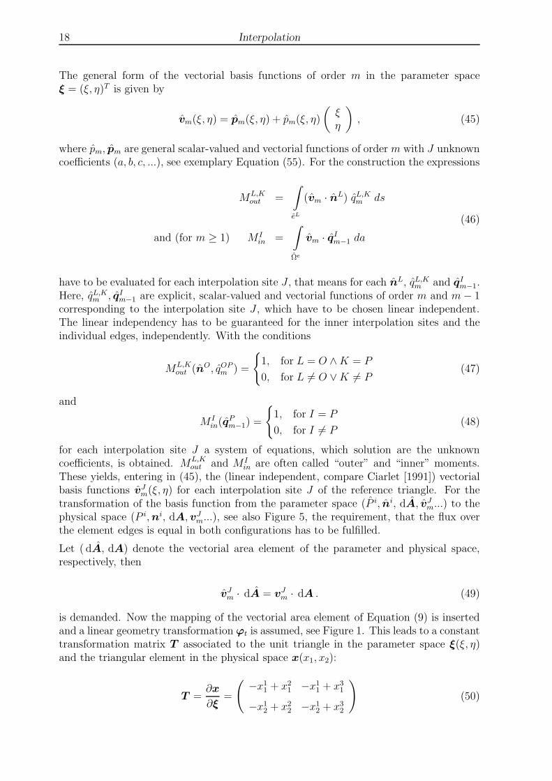
The interpolation order as well as the number of interpolation sites for a two-dimensionaltriangular element up to order m = 3 is given in Table 1. In the framework of this contri-bution the derivations are restricted to meshes with non-curved edges. An enhancementto curved boundaries has been done in Bertrand et al. [2014].
RTm Pol. order of ΨJm |Jout|C per eL |Jout|C |J in|C |J |C
RT0 linear 1 3 0 3
RT1 quadratic 2 6 2 8
RT2 cubic 3 9 6 15
RT3 quartic 4 12 12 24
Table 1: Raviart-Thomas setups (m = 0, 1, 2, 3) in two dimensions.
18 Interpolation
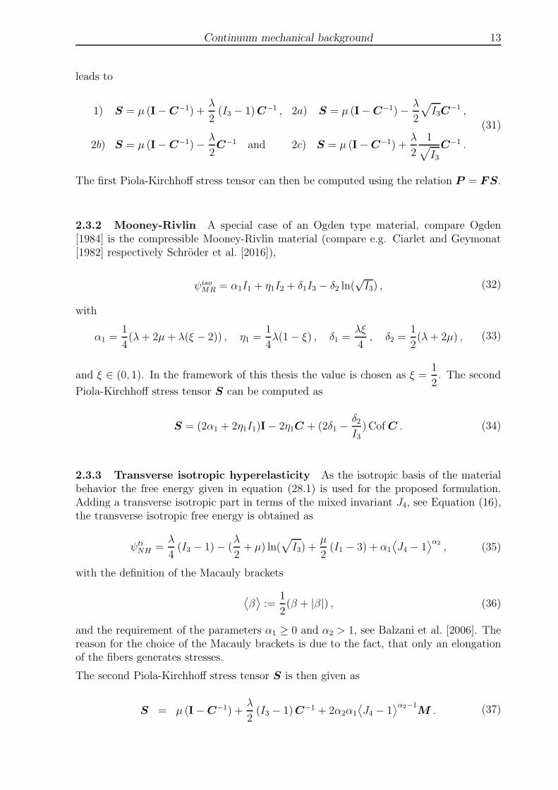
The general form of the vectorial basis functions of order m in the parameter spaceξ = (ξ, η)T is given by
vm(ξ, η) = pm(ξ, η) + pm(ξ, η)
(ξη
)
, (45)
where pm, pm are general scalar-valued and vectorial functions of order m with J unknowncoefficients (a, b, c, ...), see exemplary Equation (55). For the construction the expressions
ML,Kout =
∫
eL
(vm · nL) qL,Km ds
and (for m ≥ 1) M Iin =
∫
Ωe
vm · qIm−1 da
(46)
have to be evaluated for each interpolation site J , that means for each nL, qL,Km and qIm−1.
Here, qL,Km , qIm−1 are explicit, scalar-valued and vectorial functions of order m and m− 1
corresponding to the interpolation site J , which have to be chosen linear independent.The linear independency has to be guaranteed for the inner interpolation sites and theindividual edges, independently. With the conditions
ML,Kout (nO, qOP
m ) =
1, for L = O ∧K = P
0, for L 6= O ∨K 6= P(47)
and
M Iin(q
Pm−1) =
1, for I = P
0, for I 6= P(48)
for each interpolation site J a system of equations, which solution are the unknowncoefficients, is obtained. ML,K
out and M Iin are often called “outer” and “inner” moments.
These yields, entering in (45), the (linear independent, compare Ciarlet [1991]) vectorialbasis functions vJ
m(ξ, η) for each interpolation site J of the reference triangle. For thetransformation of the basis function from the parameter space (P i, ni, dA, vJ
m...) to thephysical space (P i,ni, dA, vJ
m...), see also Figure 5, the requirement, that the flux overthe element edges is equal in both configurations has to be fulfilled.
Let ( dA, dA) denote the vectorial area element of the parameter and physical space,respectively, then
vJm · dA = vJ
m · dA . (49)
is demanded. Now the mapping of the vectorial area element of Equation (9) is insertedand a linear geometry transformation ϕt is assumed, see Figure 1. This leads to a constanttransformation matrix T associated to the unit triangle in the parameter space ξ(ξ, η)and the triangular element in the physical space x(x1, x2):
T =∂x
∂ξ=
(−x11 + x21 −x11 + x31
−x12 + x22 −x12 + x32
)
(50)

Interpolation 19
P 2ξ
P 1
n2
n3
e3
e2
n1
e3
e2
P 3
P 2
n2
n1
n3
e1
e1
P 3
P 1
η y
x
T
v
A
divξ
ξCof T(Cof T )−T
det[T ]−1v
A
divx
x
Ωe
Ωe
Figure 5: Piola transformation.
with the known coordinates of the vertices P I = (xI1, xI2) in the physical space. With this
in hand and Cof T = det[T ]T−T
vJm = Cof[T ]TvJ
m vJm =
1
detTT vJ
m (51)
is obtained from Equation (49), which transforms the basis function of the parameterspace vJ
m to the basis function of the physical space vJm. Furthermore, the divergence of
the basis function has to be transformed. Applying the divergence with respect to thephysical space (divx) on both sides of (51) yields
divxvJm = divx[
1
detTT vJ
m] =1
detTdivξv
Jm, (52)
using the relations
TdivxvJm = divξv
Jm and divx[
1
detTT ] = 0 , (53)
because T is a constant matrix. To obtain the vector-valued Raviart-Thomas interpolationfunctions ΨJ
m, a normalization condition on vJm has to be applied in order to get suitable
functions for ΨJm.
The sum of all Raviart-Thomas shape function ΨJm belonging to one edge multiplied
with the associated normal of this edge should be equal to one.
It should be remarked, that a reasonable choice of the functions qL,Km , which is recom-mended by the author, simplifies the generalization of the normalization condition for allinterpolation orders m to

20 Interpolation
ΨJm = l vJ
1 and div ΨJm = l div vJ
1 , (54)
where l denotes the associated length of the edge of the interpolation site under consid-eration. In the following the construction of the interpolation functions for m = 1 will beprovided. The basic equations for the construction of m = 2 and m = 3 is given in theAppendix (see Chapter A.1 and Chapter A.2). For the construction for m = 0 the readeris referred e.g. to Schwarz [2009].
3.3.1 Basis functions for order m = 1. The general form of the vectorial basisfunction (45) for the order m = 1 is given as
v1(ξ, η) =
(a1 + a2ξ + a3ηb1 + b2ξ + b3η
)
︸ ︷︷ ︸
p1
+ (c1ξ + c2η)︸ ︷︷ ︸
p1
(ξη
)
. (55)
Since m ≥ 1, both parts of (46) have to be evaluated for the interpolation sites J = 1..8leading to eight equations
ML,Kout with L = 1..3, K = 1..2 and M I
in with I = 1..2 . (56)
Exemplary the evaluation for the sites J = 3 (M1,1out) and J = 8 (M2
in) will be consideredin more detail, see Figure 6.
J = 1,M3,1out
J = 4,M1,2out
J = 2,M3,2out
J = 5,M2,1out
ξ
η
J = 6,M2,2out
J = 3,M1,1out
J = 7,M1
in
J = 8,M2
in
Figure 6: Numbering of interpolation sites J for RT1.
The complete set of functions qL,K1 and qI0 and neccesary additional conditions (correlation
of coordinates) for the construction of RT1 are given in Table 2.

Interpolation 21
L K I qL,K1 / qI0 correlation of coordinates
1 1 - 2ξ η = 1− ξ
1 2 - 2η η = 1− ξ
2 1 - 2η ξ = 0
2 2 - 2(1− η) ξ = 0
3 1 - 2(1− ξ) η = 0
3 2 - 2ξ η = 0
- - 1 (1, 0)T -
- - 2 (0, 1)T -
Table 2: Set of functions qL,K1
and qI0 and correlation of coordinates for the construction
of RT1.
J = 3, M1,1out: Evaluating the first part of (46) with n1 =
√
1
2
(11
)
, q1,11 = 2ξ and the
correlation for the coordinates ξ + η = 1 leads to
M1,1out =
∫
e1
(v1 · n1) q1,11 ds
=
∫
e1
(a1 + a2ξ + a3η + c1ξ
2 + c2ξηb1 + b2ξ + b3η + c1ξη + c2η
2
)
· 1√2
(11
)
2ξ ds
= a1 +2a23
+a33
+ b1 +2b23
+b33+
2c13
+c23,
(57)
with ds =√2dξ.
J = 8, M2in: For this interpolation site q2
0 = (0, 1)T is chosen and, evaluating the secondpart of (46),
M2in =
∫
Ωe
vm · q20 da
=
1∫
0
1−η∫
0
(a1 + a2ξ + a3η + c1ξ
2 + c2ξηb1 + b2ξ + b3η + c1ξη + c2η
2
)(01
)
dξdη
=b12+b26+b36+c124
+c212,
(58)
is obtained. The computations at each interpolation site, as exemplary done for J = 3 inEquation (57) and J = 8 in Equation (58), yields under consideration of (47) and (48) asystem of equations, which has to be solved for each interpolation site J . The right-hand
side vector has a non-vanishing entry at the Jth entry, which is equal to one. Solving

22 Interpolation
the system of equations yield the parameter ai, bi for i = 1, 2, 3 and c1, c2 of the vectorialbasis functions (55) in the form (a1, a2, a3, b1, b2, b3, c1, c2)
T . We obtain the coefficients forthe eight vectorial basis functions vJ
1 for the considered RT1-case as given in Table 3.
v11 v21 v31 v41 v51 v61 v71 v81
a1 0 0 0 0 1 −2 0 0
a2 3 −2 −2 −1 −1 6 16 8
a3 0 0 0 0 −3 3 0 0
b1 −2 1 0 0 0 0 0 0
b2 3 −3 0 0 0 0 0 0
b3 6 −1 −1 −2 −2 3 8 16
c1 −4 4 4 0 0 −4 −16 −8
c2 −4 0 0 4 4 −4 −8 −16
Table 3: Set of coefficients for the construction of RT1.
Now the obtained vector-valued basis functions (as well as their divergences) has to betransformed to the physical space by Equation (51) and Equation (52) and normalizedby Equation (54).
3.4 Alternative discretization of W q(div,B)
It is inconvenient if the nodal degree of freedom respectively the nodal quantity is notequal to the interpolated quantity at this position. Consequently, the nodal results comingfrom the sytem of equations does not have any physical meaning, which is, at leastfrom an engineering point of view, unsatisfying. Especially if the nodal values are usedfor postprocessing or for non-constant boundary conditions this property is desirable.Unfortunately, the latter described way of construction does not demand the interpolationfunction to be one at its nodal coordinates and zero at all other nodes. This leads, form ≥ 2, to vector-valued functions, which does not fulfill the condition.
To show this effect, exemplary for RT2, the interpolation functions are evaluated on a unittriangular domain. In detail the functions are considered for the edge e3 or rather e3, as forthe used unit traingle Ωe = Ωe. In Figure 7 it can be seen, that the constructed functionshave their roots not at the coordinates of the respective interpolation site. Furthermore,the functions are not one at their respective nodes. It should be remarked that this factdoes not influence the correctness of the discretization.
In order to overcome this issue, the aim is to develop alternative interpolation functions ofRaviart-Thomas type, which fulfill this condition. For the latter approach the evaluationof the outer and inner moments lead to the sought functions. In contrast to that, thealternative approach uses a nodal evaluation of a prescribed condition. Therefore, it hasto be started from the general form given in Equation (45) respectively Equation (55),Equation (135) and Equation (137). Now for each outer interpolation site the functionsvJm are sought, which fulfill, multiplied with their associated normal nL and the length lL
of the associated site eL, the nodal condition

Interpolation 23
-1.00
-0.50
0.00
0.50
1.00
1.50
0 0.2 0.4 0.6 0.8 1
ΨJ 2
e3
-1.00
-0.50
0.00
0.50
1.00
1.50
0 0.2 0.4 0.6 0.8 1
ΨJ 2
e3
Ψ12
Ψ22
Ψ32
Ψ12
Ψ22
Ψ32
Figure 7: Plot of the Raviart-Thomas functions ΨJ2over the edge e3 on a unit triangular
domain
vJm(ξI , ηI) · nLlL =
1, for I = J
0, for I 6= J .(59)
For the inner nodes
vJm · qI
m−1 =
1, for I = J
0, for I 6= J(60)
has to be evaluated. The vectorial functions qIm−1 can be chosen as given in Table 2,
Table 10 and Table 13. This leads to J systems of equations which have to be solved inorder to find the unknown coefficients. Entering in (45) yields the basis functions whichnow have to be Piola transformed, see Equation (51) and Equation (52).
-3.00
-2.00
-1.00
0.00
1.00
2.00
3.00
0 0.2 0.4 0.6 0.8 1
ΨJ 2
e3
-3.00
-2.00
-1.00
0.00
1.00
2.00
3.00
0 0.2 0.4 0.6 0.8 1
ΨJ 2
e3
Ψ12
Ψ22
Ψ32
Ψ12
Ψ22
Ψ32
Figure 8: Plot of the alternative Raviart-Thomas functions ΨJ2over the edge e3 on a unit
triangular domain

24 Interpolation
Furthermore, they have to be normalized, see Equation (54), in order to obtain the vector-valued Raviart-Thomas interpolation functions ΨJ
m as well as their divergence div ΨJm.
Again, exemplary for edge e3, the roots of the functions as well as the point, wherethe functions evaluate to be one can be seen, which is now at the nodal coordinates forthis alternative basis functions, see also Figure 8. The coefficients for the vectorial basisfunctions for m = 1, m = 2 and m = 3 are given in a tabular form in the Appendix, seethe chapters A.3, A.4 and A.5. In Figure 9 several vector-valued basis functions of RT2are plotted over the unit triangular domain. Here it becomes viewable, that the normalsof the basis functions vanish at the edges, which are not associated with the interpolationsite. For the inner nodes all normals to the edges of the basis functions vanish.
J = 3 J = 6
J = 7 J = 14
Figure 9: Plot of the basis functions v3
2, v6
2, v7
2and v14
2.

The least-squares mixed finite element method 25
4 The least-squares mixed finite element method
In this chapter the construction of least-squares functionals and the variations of a func-tional for finding the minimum are considered. Besides the general approach, a least-squares setup for hyperelastic materials described by free energy functions is provided.Furthermore, for a deeper understanding of the method, a one-dimensional introductoryexample is discussed, where all steps starting from the differential equation and the least-squares functional up to the solution of a simple boundary value are shown in detail. Inaddition to that, some remarks will be given concerning the boundary conditions and theimplementation. Finally, all used element types will be presented. For the details onthe standard tasks of the finite element method, as e.g. discretization, transformation,integration and assembly the reader is referred to state of the art FEM textbooks ase.g. Bathe [1995], Zienkiewicz and Taylor [2000], Wriggers [2001], Zhu et al. [2005] andBelytschko et al. [2000].
4.1 Construction of least-squares functionals
An advantage of the least-squares method is the flexibility to design suited functionalsdirectly approximating the unknown field variables of interest. Hence, the first step isthe construction of a functional containing the governing equations. In general there aredifferent possibilities, e.g. different norms, in order to define a least-squares functional,see Bochev and Gunzburger [2009]. In this contribution a squared L2(B)-norm is used forthe construction, formally given by
||a||2L2(B) =
∫
B
|a|2 dV . (61)
In order to define the minimization problem, the squared L2(B)-norm is applied directlyto a first-order system of i differential equations written in residual forms Ri = 0, as
F(U) =∑
i
1
2||ωiRi||2L2(B) =
∑
i
∫
B
1
2ω2i Ri •Ri dV → min , (62)
with the weights ωi and the vector of unknown fields U . Here, the general scalar productof two quantities is denoted by “ • ”. In order to find the unknowns Uj which minimize thefunctional F(U), the variational calculus is used. Thus, the first variations with respectto the vector of unknown fields U have to vanish, i.e.
δUjF =
∂F∂Uj
δUj =∑
i
∫
B
ω2i δUj
Ri •Ri dV = 0 . (63)
In case of linear elasticity, the discretized form of (63) directly yields a linear systemof algebraic equations. In case of non-linearities, iterative procedures as for example astandard Newton scheme can be used in order to obtain the final solution. Therefore, the

26 The least-squares mixed finite element method
second variation has to be provided as
∆UkδUj
F =∂(δUj
F)
∂Uk
∆Uk =∑
i
∫
B
ω2i (∆Uk
δUjRi •Ri + δUj
Ri •∆UkRi) dV. (64)
The general concept of finite element methods enables to solve differential equations onarbitrary domains. Therefore, the domain of consideration B has to be discretized into afinite number of polygonal elements Be. The approximated Bh domain is then given asthe union of the finite element domains
B ≈ Bh =
nele⋃
e=1
Be , (65)
with nele denoting the number of elements. The resulting functional (as well as thevariations) are then given as the sum of the functional (variations) evaluated on eachfinite element,
F =
nele∑
e=1
F e , δF =
nele∑
e=1
δF e and ∆δF =
nele∑
e=1
∆δF e , (66)
with F e (δF e, δ∆F e) denoting the contribution of a typical element.
4.2 General setup for the hyperelastic least-squares formulation
For the development of a hyperelastic least-squares formulation, the general rules de-scribed in Chapter 4.1 are used. The formulation of consideration uses the displacementsu and the first Piola-Kirchhoff stresses P as unknowns yielding the vector of unknownfields U = (u,P )T . As a starting point for the construction of a least-squares functionalfor hyperelasticity the residuals
R1 = DivP + f = 0 → balance of momentum ,
R2 = P − ρ0∂Fψ(C) = 0 → constitutive relation ,
R3 = F−1P − (F−1P )T = 0 → stress symmetry
(67)
are defined, where f denotes the body force. From the mathematical point of view thethird residual is redundant and could be neglected, which has been proven by Cai andStarke [2004] for the linear elastic case, since the constitutive relation with its associatedresidual takes care of the fulfillment of this property. However, from a practial point ofview it seems to be advantageous to control the lack of symmetry of the stress quantity(associated to the balance of moment of momentum) directly, see e.g. Schwarz et al.[2014]. Following (62), a general least-squares functional for hyperelasticity with thesolution quantities displacements and first Piola-Kirchhoff stress tensor for one element

The least-squares mixed finite element method 27
is obtained as
F e(P ,u) =1
2
∫
Be
ω21(DivP + f ) · (DivP + f ) dV
+1
2
∫
Be
ω22(P − ρ0∂Fψ(C)) : (P − ρ0∂Fψ(C)) dV
+1
2
∫
Be
ω23(F
−1P − (F−1P )T ) : (F−1P − (F−1P )T ) dV .
(68)
For the minimization the first variations needs to be zero leading to
δuF e =3∑
i=1
∫
Be
ω2i δuRi •Ri dV = 0 ,
δPF e =3∑
i=1
∫
Be
ω2i δPRi •Ri dV = 0 ,
(69)
with
δu = 0 on ∂Bu and δP = 0 on ∂BP . (70)
The linearization for the application of a Newton scheme yields
∆uδuF e =3∑
i=1
∫
Be
ω2i (∆uδuRi •Ri + δuRi •∆uRi) dV ,
∆P δuF e =3∑
i=1
∫
Be
ω2i (∆P δuRi •Ri + δuRi •∆PRi) dV ,
∆uδPF e =3∑
i=1
∫
Be
ω2i (∆uδPRi •Ri + δPRi •∆uRi) dV ,
∆P δPF e =3∑
i=1
∫
Be
ω2i (∆P δPRi •Ri + δPRi •∆PRi) dV .
(71)
The non-trivial variations are given by
δPR1 = Div δP ,
δuR2 = −ρ0∂2FFψ(C)δF , δPR2 = δP ,
δuR3 = δF−1P − (δF−1P )T ,
δPR3 = F−1δP − (F−1δP )T
(72)
and the associated linear increments appear as
∆PR1 = Div∆P ,
∆uR2 = −ρ0∂2FFψ(C)∆F , ∆PR2 = ∆P ,
∆uR3 = ∆F−1P − (∆F−1P )T ,
∆PR3 = F−1∆P − (F−1∆P )T .
(73)

28 The least-squares mixed finite element method
The non-vanishing terms for the second variation are
∆uδuR2 = −∂F (∂2FFψ(C)δF )∆F ,
∆uδuR3 = ∆δF−1P − (∆δF−1P )T ,
∆P δuR3 = δF−1∆P − (δF−1∆P )T ,
∆uδPR3 = ∆F−1δP − (∆F−1δP )T .
(74)
4.3 Interpolation of field quantities
Both unknown fields have to be suitably interpolated. For convenience and generality inthe following interpolation matrices are introduced. For details on the used interpolationspaces and the interpolation functions see Chapter 3 and for the resulting different elementtypes see Chapter 4.5. First, the displacement vector u, the related test function δu andthe related increment ∆u are introduced. It is obtained with the interpolation matrix N
u =∑
I
N I du I , δu =
∑
I
N Iδ du I and ∆u =
∑
I
N I∆du I , (75)
with the nodal displacement vector du I and the interpolation sites for the displacement
denoted by I. The displacement gradient is then interpolated by
∇u =∑
I
BI du I , ∇δu =
∑
I
BIδ du I and ∇∆u =
∑
I
BI∆du I , (76)
where B contains the derivatives of the interpolation functions. The first Piola-Kirchhoffstress tensor is interpolated as
P =∑
J
AJ dP J , δP =∑
J
AJδ dP J and ∆P =∑
J
AJ∆dP J , (77)
with A denoting the suitable interpolation matrix for the interpolation of the stresses anddP J denoting the nodal degrees of freedom of the stresses at each stress interpolation siteJ . The divergence of the first Piola-Kirchhoff stress tensor is obtained by
DivP =∑
J
DAJ dP J . (78)
The detailed structure of the presented interpolation matrices is dependent on the el-ement type used and is shown in Chapter 4.5.2. In the next subsection, for a deeperunderstanding of the method, an illustrative one-dimensional example for a mixed prob-lem exploiting all steps in detail for the treatment of a boundary value problem with theLSFEM is provided.

The least-squares mixed finite element method 29
4.4 Introductory example in 1D
For a deeper understanding of the method an easy application of the mixed least-squaresfinite element method in one dimension is taken under consideration. Here, for conve-nience, our notation for the used quantities is simplified to
P1D−→ P11 −→ P
DivP1D−→ P11,1 −→ P ′
f1D−→ f1 −→ f
F = I+∇u1D−→ F11 = δ11 + u1,1 −→ F = 1 + u′
C = F TF1D−→ C11 = F11F11 −→ C = F 2
(79)
In 1D, the derivative of the displacement u yields the strain u′. We start from the balanceof linear momentum, an elliptic differential equation of second order (in u), given as
(P (u′))′ + f = 0 (80)
on a domain B, where P is a function of the derivative of the displacements. For thesuitable interpolation of u, C1 continuous functions have to be chosen, since second-orderderivatives of u arise in the differential equation. In order to circumvent this and enablingthe use of C0 continuous interpolation functions, the differential equation of second orderis transformed into a system of differential equations of first order. Therefore, the stressesare introduced as an additional unknown field and a further residual equation describingthe relation between stresses and strains is added. This relation is given by the constitutivelaw. Here, P is given as the derivative of a function
ψ = (λ
4+µ
2) (F 2 − 1)− (
λ
2+ µ) ln(F ) , (81)
which is comparable to the free energy presented in Section 2.3.1, Equation (28.1) un-der the assumption of no transversal contraction (Poisson’s ratio ν = 0) leading to amaterial parameter λ = 0. Nevertheless, λ is maintained in the derivation for the sakeof completeness. Differentiating (81) with respect to F yields the (first Piola-Kirchhoff)stresses
P = ∂Fψ = (λ
2+ µ)(F − 1
F) . (82)
The nonlinear material behavior is depicted as a “stress-strain”- curve (chosing λ = 0, µ =1), see Figure 10. The first-order system in residual form is obtained as
R1 = P ′ + f = 0 and R2 = P − (λ
2+ µ)(F − 1
F) = 0 (83)
with the boundary conditions
u = g on ∂Bu ⊆ ∂B and P = h on ∂BP ⊆ ∂B (84)

30 The least-squares mixed finite element method
-10.00
-8.00
-6.00
-4.00
-2.00
0.00
2.00
-1 -0.8 -0.6 -0.4 -0.2 0 0.2 0.4 0.6 0.8 1
P
u′
Figure 10: Stress-strain- curve (λ = 0, µ = 1), 1D.
and the decomposition
∂B = ∂Bu ∪ ∂BP ∧ ∂Bu ∩ ∂BP = ∅ . (85)
Applying a squared L2(B)-norm and a weighting for the residuals leads to the least-squaresfunctional
F =1
2||ω1R1||2L2(B) +
1
2||ω2R2||2L2(B)
=1
2
∫
B
ω21R2
1 dX +1
2
∫
B
ω22R2
2 dX → min ,
(86)
which has to be minimized. Thus, the first variations δuF and δPF with respect to thesolution variables (u, P ) have to be zero. With δF = δu′ Equation (63) yields
δuF = ω22
∫
B
δuR2 R2 dX = 0 ,
δPF = ω21
∫
B
δPR1 R1 dX + ω22
∫
B
δPR2 R2 dX = 0 ,
(87)
with
δuR2 = −δF(λ
2+ µ
)(
1 +1
F 2
)
, δPR1 = δP ′ and δPR2 = δP (88)
and the conditions
δu = 0 on ∂Bu and δP = 0 on ∂BP . (89)

The least-squares mixed finite element method 31
Since (87) is nonlinear (the terms R2 and δuR2 are broken rational in u′), a Newtonscheme is applied to find the root. Therefore, the non-zero second variations of (64) aregiven as
∆uδuF = ω22
∫
B
∆uδuR2 R2 + δuR2 ∆uR2 dX ,
∆P δuF = ω22
∫
B
δuR2 ∆PR2 dX ,
∆uδPF = ω22
∫
B
δPR2 ∆uR2 dX ,
∆P δPF = ω21
∫
B
δPR1 ∆PR1 dX + ω22
∫
B
δPR2 ∆PR2 dX ,
(90)
with the terms
∆uδuR2 = δF
(λ
2+ µ
)2
F 3∆F , ∆uR2 = −
(λ
2+ µ
)(
1 +1
F 2
)
∆F ,
∆PR1 = ∆P ′ and ∆PR2 = ∆P ,
(91)
with ∆F = ∆u′. For the discretization mixed finite elements are used consisting of acombination of a quadratic three-noded element (for u) and a linear two-noded element(for P ) with one degree of freedom at each node. This leads to a reference element inthe parameter space (ξ) with three nodes. Here, the first two nodes have two degrees offreedom and the midnode has one degree of freedom, see Figure 11.
1ξ
1 1ξ
1
dP 2dP 1du 1 du 2du 3
1ξ
1
X1, du 1, dP 1 X2, du 2, dP 2X3, du 3
Figure 11: Mixed reference element (Ωe) in 1D.
The vectors of the nodal degrees of freedom for u, P and the geometry X are given as
du = [ du 1, du 2, du 3]T , dP = [ dP 1, dP 2]T and X = [X1, X2, X3]T . (92)
For the approximation of the unknown field u and the geometry X quadratic polynomialinterpolation on the reference element Ωe = [−1, 1] is used with the shape functionssummarized in a vector Nu,

32 The least-squares mixed finite element method
Nu(ξ) = [N1u , N
2u , N
3u ] =
[1
2(ξ2 − ξ),
1
2(ξ2 + ξ), 1− ξ2
]
(93)
and the corresponding vector Bu(ξ) = ∂XNu(ξ) containing the derivatives of the shapefunctions with respect to X
Bu(ξ) = [B1u, B
2u, B
3u] =
2
le
[
ξ − 1
2, ξ +
1
2, −2ξ
]
. (94)
Here, the derivatives of the shape functions are derived by the chain rule
∂N
∂X=∂N
∂ξ
∂ξ
∂X=∂N
∂ξJ−111 (95)
with the transformation J11. With X = (0, le, le/2)T
J11 =∂X
∂ξ=
3∑
I=1
N Iu,ξX
I = (ξ − 1
2)0 + (ξ +
1
2)le − (2ξ)
le
2=le
2(96)
is obtained. With the element nodes I = 1, 2, 3 the interpolation of u′ and the variationsδF , ∆F are given by
u′(ξ) = Bu(ξ)du , δF (ξ) = δu′(ξ) = Bu(ξ)δ d
u , ∆F (ξ) = ∆u′(ξ) = Bu(ξ)∆du (97)
and the geometry approximation is
X(ξ) = Nu(ξ)x . (98)
For the approximation of P polynomial interpolation of order one on the reference elementdomain Ωe = [−1, 1] is chosen. The choice of a linear approach for P is reasonable. Thisis based on the quadratic interpolation of u, the resulting interpolation order of u′ andits relation to P . Here, the free choice of the interpolation orders for the unknowns ispossible due to the fact, that least-squares mixed finite elements are not restricted to theLBB-condition, unlike e.g. mixed Galerkin elements compare for instance Jiang [1998],Bochev and Gunzburger [2009] and Braess [1997]. The vector of the shape functions offirst order NP appears as
NP (ξ) = [N1P , N
2P ] =
[1
2(1− ξ),
1
2(1 + ξ)
]
. (99)
The vector of the derivatives of the shape functions BP (ξ) = ∂XNP (ξ) has the form
BP (ξ) = [B1P , B
2P ] =
2
le
[
−1
2,1
2
]
. (100)

The least-squares mixed finite element method 33
With the interpolation of P , P ′ and their variations δP and δP ′, the matrix expressionsare obtained as
P (ξ) =
2∑
J=1
NJP d
P J = NP dP , δP (ξ) =
2∑
J=1
NJP δ d
P J = NP δ dP,
P ′(ξ) =2∑
J=1
BJP d
P J = BP dP , δP ′(ξ) =2∑
J=1
BJP δ d
P J = BP δ dP
(101)
The domain is discretized with nele finite elements, i.e. B = Bh =
nele⋃
e=1
Be. The first and
the second variation follow as
δF = δuF + δPF =∑
e
δF e and
∆δF = ∆uδuF +∆uδPF +∆P δuF +∆P δPF =∑
e
∆δF e
(102)
with the contributions of a typical element
δF e = δ du T
∫
Be
−BTu ω
22
(λ
2+ µ
)
(1 +1
F 2)R2 dx
︸ ︷︷ ︸
reu
+ δ dP T
∫
Be
BTP ω
21 R1 +NT
P ω22 R2 dx
︸ ︷︷ ︸
reP
(103)and
∆δF e = δ du T
∫
Be
BTu
[
ω22
(λ
2+ µ
)2
F 3R2 + ω2
2
((λ
2+ µ
)
(1 +1
F 2)
)2]
Bu dx
︸ ︷︷ ︸
Keuu
∆du
− δ du T
∫
Be
BTu
[
ω22
((λ
2+ µ
)
(1 +1
F 2)
)]
NP dx
︸ ︷︷ ︸
KeuP
∆dP
− δ dP T
∫
Be
NTP
[
ω22
((λ
2+ µ
)
(1 +1
F 2)
)]
Bu dx
︸ ︷︷ ︸
KePu
∆du
+ δ dP T
∫
Be
BTP ω
21 BP +NT
P ω22 NP dx
︸ ︷︷ ︸
KePP
∆dP.
(104)

34 The least-squares mixed finite element method
Here, Keuu,K
euP ,K
ePu,K
ePP denote the submatrices of the element stiffness matrix Ke
and reu and re
P denotes the entries of the element right-hand-side vector re. This leads tothe system of equations for one element of the form
Keuu Ke
uP
KePu Ke
PP
︸ ︷︷ ︸
Ke
∆du e
∆dP e
︸ ︷︷ ︸
∆de
= −
reu
reP
︸ ︷︷ ︸
re
, (105)
with the element vector of the increments of the degrees of freedom ∆de = [∆du e, ∆d
P e]T .The transformation of the integral from the physical space (here dx) to the referencedomain Ωe = [−1, 1] (here dξ) is based on
∫
Be
dx =
∫
Ωe
J11 dξ , (106)
where the Jacobian J11 given in (96). The evaluation of the integral expressions can bedone analytically or, as mostly used in the field of finite element formulations by numer-ical integration schemes as, for instance, Gaussian quadrature, see e.g. Wriggers [2001].Transformation and evaluation of the integral leads to a nonlinear system of equationswhich can be solved using a Newton scheme.As a simple example, a one-dimensional boundary value problem with essential displace-ment boundary conditions on both sides (u(0) = u(l) = 0) and a bodyforce f = 2 isconsidered, compare Figure 12. The domain is discretized by one element with an el-
l = 1
x
f = 2
Figure 12: Setup boundary value problem in 1D.
ement length of le = l = 1. The material parameters are chosen as λ = µ = 1 andthe weights as ω1 = ω2 = 1. Due to the essential boundary conditions for the displace-ments, du 1 = du 2 = 0. The initial values for the Newton iteration are given as zero for allremaining nodal degrees of freedom
dred,0 = [ du 30, d
P 10, d
P 20]
T = 0 (107)
and will be updated as
dred,n+1 = dred,n +∆dred(108)

The least-squares mixed finite element method 35
after each Newton step. Since only one element is considered, no assembly procedure isnecessary. The resulting reduced system of equations (due to the boundary conditionsand (89)) reads
48 −2 2
−24
3−5
6
2 −5
6
4
3
︸ ︷︷ ︸
Kred
∆ du 3
∆ dP 1
∆ dP 2
︸ ︷︷ ︸
∆dred
= −
0
−2
2
︸ ︷︷ ︸
rred
, (109)
with the reduced stiffness matrix Kred, the increments of the reduced vector of degrees offreedom ∆dred and the reduced right-hand-side vector rred. The increments of the degreesof freedom as well as the updated ones for each Newton iteration (NI) are obtained as
NI ∆dred dred
0 [0, 0, 0]T [0, 0, 0]T
1 [0.0833333, 1.,−1.]T [0.0833333, 1.,−1.]T
2 [−0.00147549,−0.055534,−0.0556075]T [0.0818578, 0.944466,−1.05561]T
3 [−39.1677,−3.15172, 70.2618]T×10−6 [0.0818187, 0.944463,−1.05554]T
4 [−3.56342,−12.5686,−7.70844]T×10−9 [0.0818187, 0.944463,−1.05554]T
(110)
and the residual norms |rred| at the end of each Newton iteration yields
NI |rred|
0 2.82843
1 0.169474
2 0.0019758
3 2.02438× 10⁻⁷
4 2.23428× 10⁻¹⁵
(111)
The solution of the Newton iteration yields dred = [0.0818187, 0.944463,−1.05554]T . Forcomparison the differential equation of second order
(λ
2+ µ
)(
u′′(X) +u′′(X)
1 + u′(X)2
)
+ 2 = 0 (112)

36 The least-squares mixed finite element method
resulting from (80) with (79) and (81) on the domain X = [0, 1] with the boundaryconditions u(0)=u(1)=0 is solved using the command NDSolve of Mathematica (where“Explicit Euler” is chosen as the method). This leads to the result u(0.5) = 0.0818432,u′(0) = 0.363335 → P (0) = 0.94476 and u′(1) = −0.291704 → P (1) = −1.05532.Furthermore, the result for a discretization with ten least-squares elements compared tothe numerical solution of Mathematica is shown in Figure 13. It can be concluded, thatthe provided least-squares mixed finite element formulation is able to solve the givendifferential equation of second order in an appropriate way.
0.00
0.01
0.02
0.03
0.04
0.05
0.06
0.07
0.08
0 0.2 0.4 0.6 0.8 1
u
x
LSMMathematica
Figure 13: Solution for the displacements u, Mathematica vs LSM, 1D.
4.5 Different least-squares element types under investigation
Considering solid materials, the displacement field is, under some technical assumptions(e.g. no cracks), in general continuous. Hence, an approximation in the space W 1,p(B)is a suitable choice, as it ensures continuity of the overall interpolated field from elementto element. Therefore, standard interpolation polynomials are chosen for the approxima-tion of the displacements. The solution for the stresses can naturally be found in theSobolev space W q(div,B). This is due to the fact, that stresses are normal continuous,see also Figure 2. That means, that the normal entries of the stresses, which can bedenoted by the so-called traction vector (t = σn, T = PN) are continuous. There-fore, the choice of vector-valued Raviart-Thomas functions for the interpolation of thestresses are a suitable choice, due to their ability to ensure a conforming discretizationin W q(div,B). We obtain the approximations as
u ∈ W 1,p(B)d : u|Be
∈ Pk(Be)d; ∀ Be
andP ∈ W q(div,B)d : P |Be
∈ RTm(Be)d ∀ Be
, with d denoting the dimension. These
resulting elements of type RTmPk where m denotes the polynomial order of the stress in-terpolation and k the polynomial order of the standard interpolation polynomials for theinterpolation of the displacements has primarily been developed by Cai and Starke [2003].An alternative way might be the interpolation of the stresses in W 1,p(B). Unfortunately,due to the fact that the W 1,p(B) space is more restricted (all entries are continuous)than the W q(div,B) space (just the normal entries have to be continuous), maybe a so-

The least-squares mixed finite element method 37
lution cannot (at least locally) be found, as W 1,p(B) is a subspace of W q(div,B), see alsoEquation (113).
(Pk(B))d ⊆ RTk(B) ⊆ (dPk+1(B))d
⊆ ⊆ ⊆
(W 1,p(B))d ⊆ W q(div,B) ⊆ (L2(B))d(113)
But, because of the treatment of all restrictions in a least-squares sense, the arising er-ror might be negligible small especially for fine meshes. The approximation is given byu ∈ W 1,p(B)d : u|Be
∈ Pk(Be)d; ∀ Be
and
P ∈ W 1,p(B)d : P |Be
∈ Pk(Be)d ∀ Be
. This
element type is denoted by PmPk, where m and k indicate the interpolation order for thestresses and the displacements. Investigations in this field for a linear elastic material hasbeen done by Steeger et al. [2015]. Here, the authors mainly considered the performanceof several interpolation combinations with respect to a tip displacement. In the followingthe two-dimensional element types used in the framework of this thesis are presented.Therefore, the approximations using RT and P are considered seperately. The interpola-tions are limitted to the orders 1, 2, 3 and 4 for P and for RT to the orders 0, 1, 2 and 3.
4.5.1 Position of the interpolation sites and number of element degrees offreedom In Figure 14 the resulting elements for an interpolation using vector-valuedRaviart-Thomas interpolation functions, compare Section 3.3, are presented.
Here, the interpolation sites are denoted by arrows respectively crosses. The elementsfor the interpolation with standard interpolation polynomials are depicted in Figure 15,compare also Chapter 3.2, where the interpolation sites are denoted by bullets. Combiningthe interpolation of the displacements and the stresses yields the latter mentioned elementtypes RTmPk respectively PmPk. In Table 4 the different element types with the resultingnumber of nodes per element (nen) and the element degrees of freedom (edof) are shownin the form (nen,edof).
It becomes clear that the PmPk elements have a higher number of degrees of freedom perelement. This is due to the interpolation of the stresses in W 1,p(B), as all entries of thestress tensor are degrees of freedom, whereas for RTmPk only the entries of the local trac-tion vector are used as degrees of freedom. In Chapter 5.1 the performance of the differentelement types, with respect to the displacement approximation, under consideration of abending dominated boundary value problem is investigated. Since the difference betweenthe two element types is the interpolation space for the stresses, in Chapter 5.4 the ef-fect of different interpolation spaces for the stresses is considered. Therefore the stressdistribution over a quartered plate consisting of four different materials is computed andinvestigated, especially at the material interfaces.
4.5.2 Resulting interpolation matrices The general interpolation of the unknownfield quantities is shown in Chapter 4.3. Therefore, several interpolation matrices havebeen introduced. The detailed structure of these matrices in dependence of the element
38 The least-squares mixed finite element method
1
3
ξ
η
2
1
4
2
5
ξ
η
6
3
7, 8
ξ
η
7
10, 11
8
9
6
5
4
1 2 3
12, 13
14, 15
ξ
η
3
5
6
7
8
9
10
11
1213, 14
17, 18
15, 16
1 2 4
23, 24
19, 20
21, 22
RT0 RT1
RT2 RT3
Figure 14: Arrangement of element nodes J for RT .
(nen,edof) P1 (3, 6) P2 (6, 12) P3 (10, 20) P4 (15, 30)
P1 (3, 12) (6, 18) (9, 24) (13, 32) (18, 42)
P2 (6, 24) (9, 30) (12, 36) (16, 44) (21, 54)
P3 (10, 40) (13, 46) (16, 52) (20, 60) (25, 70)
P4 (15, 60) (18, 66) (21, 72) (25, 80) (30, 90)
RT0 (3, 6) (6, 12) (9, 18) (13, 26) (18, 36)
RT1 (8, 16) (11, 22) (14, 28) (18, 36) (23, 46)
RT2 (15, 30) (18, 36) (21, 42) (25, 50) (30, 60)
RT3 (24, 48) (27, 54) (30, 60) (34, 68) (39, 78)
Table 4: Number of element nodes (nen) and number of degrees of freedom per element(edof) for the different two-dimensional element types under consideration.
type is shown in the following under consideration of the quantity itself, as the variationand the increment are analoguously. For all vectorial quantities the structure is main-tained, whereas all tensorial quantities are restored as vectors. The matrices are given forthe three-dimensional case but can be easily reduced to the two-dimensional case.
For the interpolation of the displacement field in Equation (75) the matrixN (respectivelyB for the gradient) is introduced. As both element types use standard interpolation

The least-squares mixed finite element method 39
1
3
ξ
η
2 1
3
ξ
η
24
56
1
3
ξ
η
24
6
8
5
7
910
1
3
ξ
η
24
7
10
5
9
13
11
12
6
8
14
15
P1 P2
P3 P4
Figure 15: Arrangement of element nodes I for P .
polynomials for the interpolation of the displacement field (and its gradient) the matricesare obtained as
u =
u1
u2
u3
=∑
I
N I du I =
∑
I
N I 0 0
0 N I 0
0 0 N I
du I1
du I2
du I3
, (114)
∇u =
u1,1
u1,2
u1,3
u2,1
u2,2
u2,3
u3,1
u3,2
u3,3
=∑
I
BI du I =
∑
I
N,I1 0 0
N,I1 0 0
N,I1 0 0
0 N,I1 0
0 N,I2 0
0 N,I3 0
0 0 N,I1
0 0 N,I2
0 0 N,I3
du I1
du I2
du I3
. (115)
For the interpolation of the stress tensor it is distinguished between the different element
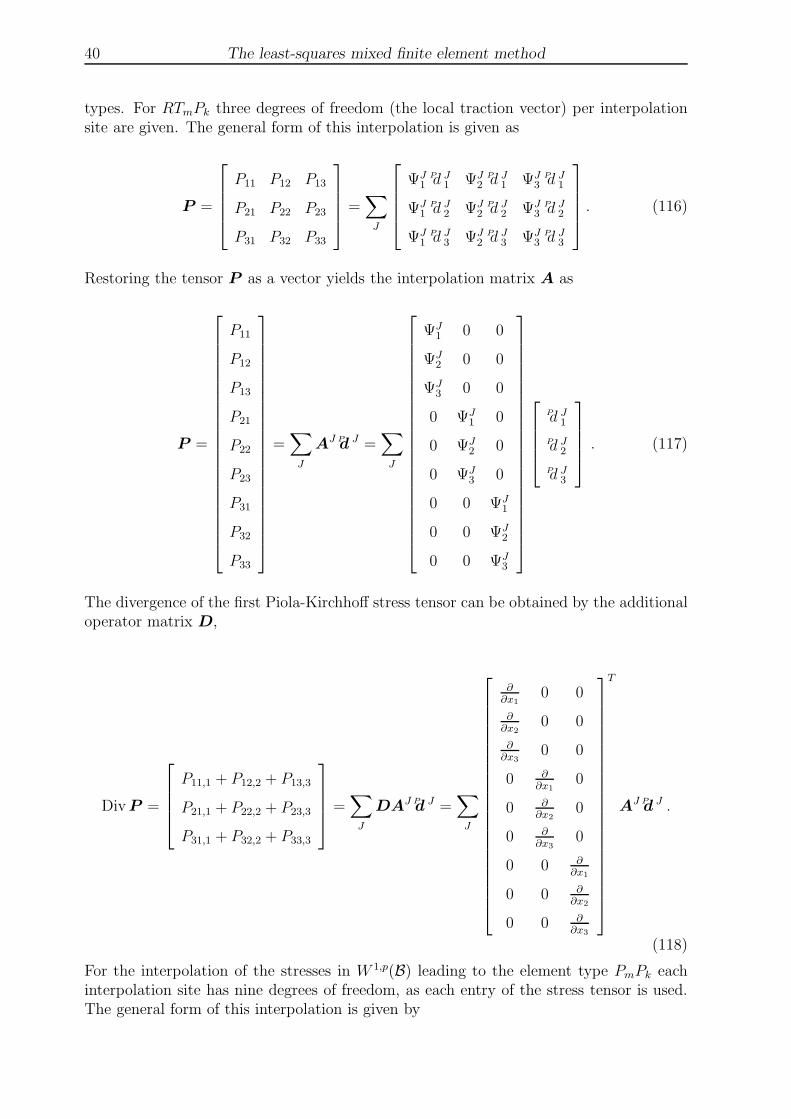
40 The least-squares mixed finite element method
types. For RTmPk three degrees of freedom (the local traction vector) per interpolationsite are given. The general form of this interpolation is given as
P =
P11 P12 P13
P21 P22 P23
P31 P32 P33
=∑
J
ΨJ1 d
P J1 ΨJ
2 dP J
1 ΨJ3 d
P J1
ΨJ1 d
P J2 ΨJ
2 dP J
2 ΨJ3 d
P J2
ΨJ1 d
P J3 ΨJ
2 dP J
3 ΨJ3 d
P J3
. (116)
Restoring the tensor P as a vector yields the interpolation matrix A as
P =
P11
P12
P13
P21
P22
P23
P31
P32
P33
=∑
J
AJ dP J =∑
J
ΨJ1 0 0
ΨJ2 0 0
ΨJ3 0 0
0 ΨJ1 0
0 ΨJ2 0
0 ΨJ3 0
0 0 ΨJ1
0 0 ΨJ2
0 0 ΨJ3
dP J1
dP J2
dP J3
. (117)
The divergence of the first Piola-Kirchhoff stress tensor can be obtained by the additionaloperator matrix D,
DivP =
P11,1 + P12,2 + P13,3
P21,1 + P22,2 + P23,3
P31,1 + P32,2 + P33,3
=∑
J
DAJ dP J =∑
J
∂∂x1
0 0
∂∂x2
0 0
∂∂x3
0 0
0 ∂∂x1
0
0 ∂∂x2
0
0 ∂∂x3
0
0 0 ∂∂x1
0 0 ∂∂x2
0 0 ∂∂x3
T
AJ dP J .
(118)
For the interpolation of the stresses in W 1,p(B) leading to the element type PmPk eachinterpolation site has nine degrees of freedom, as each entry of the stress tensor is used.The general form of this interpolation is given by

The least-squares mixed finite element method 41
P =
P11 P12 P13
P21 P22 P23
P31 P32 P33
=∑
J
NJ dP J11 NJ dP J
12 NJ dP J13
NJ dP J21 NJ dP J
22 NJ dP J23
NJ dP J31 NJ dP J
32 NJ dP J33
. (119)
Rewriting the stress tensor as a vector yields a different interpolation matrix A and adifferent vector of stress degrees of freedom as
P =
P11
P12
P13
P21
P22
P23
P31
P32
P33
=∑
J
AJ dP J =∑
J
NJ 0 0 0 0 0 0 0 0
0 NJ 0 0 0 0 0 0 0
0 0 NJ 0 0 0 0 0 0
0 0 0 NJ 0 0 0 0 0
0 0 0 0 NJ 0 0 0 0
0 0 0 0 0 NJ 0 0 0
0 0 0 0 0 0 NJ 0 0
0 0 0 0 0 0 0 NJ 0
0 0 0 0 0 0 0 0 NJ
dP J11
dP J12
dP J13
dP J21
dP J22
dP J23
dP J31
dP J32
dP J33
.
(120)
The divergence can be obtained by using Equation (118) under consideration of the matrixA of Equation (120).
4.6. Boundary conditions
For the solution of a boundary value problem, the application of boundary conditions isimportant. With the displacements u and the stresses P as field quantities, the boundarycan be divided into
∂B = ∂Bu ∪ ∂BP ∧ ∂Bu ∩ ∂BP = ∅ . (121)
In general two different kinds of boundary conditions are given, essential boundary con-ditions and natural boundary conditions. The essential boundary conditions are used forprimary variables, whereas natural boundary conditions are used for the derivative of aprimary variable. Thus for the considered least-squares mixed finite element formulation,all boundary conditions can be seen as essential ones,
u = g on ∂Bu ⊆ ∂B and P = h on ∂BP ⊆ ∂B , (122)
with vanishing variations on the boundaries,
δu = 0 on ∂Bu, δP = 0 on ∂BP . (123)

42 The least-squares mixed finite element method
The application of the displacement boundary conditions can be done as in standardsolely displacement based finite element methods. Therefore, for static analysis, all rigid-body motions have to be prevented. In the standard displacement-based FEM the zeroNeumann boundary conditions for stress-free edges (natural boundary conditions) aregenerally fulfilled apriori (due to the resulting term in the weak form). In the frameworkof the provided mixed least-squares stress-displacement formulation this is not the caseand therefore also zero-stress boundary conditions have to be defined explicitly. The actingstress at a boundary can be described by the so-called traction vector, see also Chapter2.2. For simplification the following explanations are restricted to the two dimensionalcase (x1 − x2 plane), see Figure 16, where just the positive cutting surfaces are marked.
x1
x3
x2
P22
P12
P32 P11
P21
P31
P33
P13
P23
x1
x2P22
P12
P11
P21
Figure 16: Stress state of an infinitesimal part.
With this definition of the stress tensor respectively the entries of the local tractionvector shown in Figure 16 the boundary conditions are given for a simple example forboth element types, RTmPk and PmPk.
4.6.1. Example for the application of boundary conditions As a simple examplean uniaxial tension test is considered, see Figure 17.
x1
x2
P
Figure 17: Geometry of the uniaxial tension test.
For both element types, RTmPk and PmPk the boundary conditions for the displacementsare applied via the vector of nodal displacements d
u I = ( du I1 , d
u I2 )
T . Considering this ex-

The least-squares mixed finite element method 43
ample that means that all displacement nodes on the left side are bounded in x1 directionand the node in the origin is additionally fixed in x2 direction. The upper and lower sideof the domain are stress free. Therefore, all stress nodes on the upper and lower sideyield T = PN = (P12, P22)
T = 0. For RTmPk this results in dσ I1 = dσ I
2 = 0 and forPmPk in dσ I
12 = dσ I22 = 0. On the left side only the shear stress has to be bounded, as the
normal direction is already bounded by a displacement boundary (RTmPk: dσ I2 = 0, PmPk:
dσ I21 = 0). On the right side a P11 stress is applied leading to the boundary conditions forRTmPk of dσ I
1 = P11, dσ I2 = 0 and for PmPk of dσ I
11 = P11, dσ I21 = 0. It should be remarked,
that the application of the boundary conditions for PmPk could lead to problems, as theentries of the local traction vector are, under consideration of nonrectangular domains,not equal to entries of the local stress tensor. In order to circumvent this, the stressboundaries can e.g. be applied in a least-squares sense via an additional residual whichis only defined at the stress boundaries. Therefore, in the framework of this thesis, thefunctional given in Equation (68) is extended by a boundary residual
R∂BP= PN − T = 0 (124)
to the general least-squares functional for hyperelastcity leading to
F e(P ,u) =1
2
∫
Be
ω21(DivP + f ) · (DivP + f ) dV
+1
2
∫
Be
ω22(P − ρ0∂Fψ(C)) : (P − ρ0∂Fψ(C)) dV
+1
2
∫
Be
ω23(F
−1P − (F−1P )T ) : (F−1P − (F−1P )T ) dV
+1
2
∫
∂BeP
(PN − T ) · (PN − T ) dA .
(125)
Furthermore, applying the interpolation functions of Raviart-Thomas type (RTm) givenin Chapter 3.3 could be unconvenient for m ≥ 2, as the interpolation functions are notone at its site and zero at the other sides due to the construction. Hence, for moreconvenience, the alternative functions given in Chapter 3.4 should be used.
4.7. Remarks on the implementation
In this subsection some basic remarks on the implementation are given. The detailed setupof least-squares elements is described in the internal Wiki for AceGen and AceFEM, seeAceDoc [2016]. It should be remarked, that the notation over time has changed. Hencethe notation in this thesis differs slightly from AceDoc [2016].
4.7.1. General remarks Mainly all explanations are restricted to the two-dimensionalcase. In the framework of this thesis, all given quantities as e.g. dimensions and materialparameters are denoted without any units and have to be chosen in a consistent manner(e.g. in SI units). The element implementations and computations have been done using

44 The least-squares mixed finite element method
the AceGen and AceFEM packages (version 6.503 – 6.808), see e.g. Korelc [1997; 2002]and Korelc and Wriggers [2016], of Mathematica (version 10.1–10.4), see Wolfram Re-search [2015]. Furthermore, for the visualizations Paraview (version 4.3.1), see Ahrenset al. [2005], has been used. Basis for the contour plots of the stresses are the quantitiesevaluated at the corner nodes of each triangle. Inside an element the values are inter-polated linearly, between elements the plot is discontinuous. The used mixed Galerkinelement T2P0 is based on the three field Hu-Washizu potential, compare Simo et al. [1984]
Π(u, p, θ) =
∫
B0
ψ(F ) dV +
∫
B0
p(J − θ) dV +Πext → stat.
with F = ( θJ)1/3F . The displacement u is interpolated using quadratic standard inter-
polation polynomials whereas p and θ are interpolated constant and discontinuous fromelement to element. All provided two-dimensional computations assume plain strain con-ditions.
4.7.2. General element setup in AceGen For the implementation it is distinguishedbetween nodes associated to stresses and nodes associated to displacements, even if theyare at the same coordinate. This results in the number of nodes given in Chapter 4.5,Table 4. A linear three-noded triangular element is chosen as a basis for each element(thus the provided elements are restricted to straight edges). All further nodes are addedusing the ”SMSAdditionalNodes” command, see exemplary for an RT1P2 in Figure 18.
"SMSAdditionalNodes"→Hold#1+ 2 (#2-#1)
4, #2+
2 (#3-#2)
4, #3+
2 (#1-#3)
4,
#1+#2-#1
3, #1+
2 (#2-#1)
3, #2+
#3-#2
3, #2+
2 (#3-#2)
3,
#3+#1-#3
3, #3+
2 (#1-#3)
3, #1+
#2-#1
3+#3-#1
3, #1+
#2-#1
3+#3-#1
3&
Figure 18: Adding further additional nodes using the ”SMSAdditionalNodes” commandexemplary for RT1P2.
The nodes are marked with the ”SMSNodeID” command using the denotations ”D” for adisplacement node and ”Sig” for a stress node. Each displacement node has two degreesof freedom. Each stress node for RTmPk two degrees of freedom and for PmPk four degreesof freedom. The arising integrals are solved using Gaussian quadrature with a sufficientnumber of integration points. The isoparametric concept is used, that means that for theinterpolation of the geometry the same interpolation functions as for the interpolation ofthe displacement field are used,
u =∑
I
N I du I and X =
∑
I
N IXI . (126)
After defining the necessary fields for the degrees of freedom, the kinematical quantitiesare computed, see Figure 19.

The least-squares mixed finite element method 45
u=SMSD[ux,uy,uz,dX,dY,dZ,
"Dependency"→ξ,η,ζ,dX,dY,dZ,SMSSimplify[SMSInverse[dJm]]];
SMSFreeze[F,IdentityMatrix[3]+u];
SMSFreeze[,Transpose[F].F,"Symmetric"→True];
I1,I2,I3⊨SMSInvariantsI[];
Figure 19: Computation of the kinematic quantities.
For PmPk no special treatment is neccesary for the interpolation respectively implemen-tation of the stress degrees of freedom, as all entries of the stress tensor are degrees offreedom at each node. For RTmPk it has to be taken under consideration, that the degreesof freedom are the local traction vector. Since this is dependent on the position of theelement edge of consideration, the local normal has to be computed. Unfortunately, thenormals N1,1 and N2,1 of two neighbouring elements E1 and E2 are diametrically opposed,see Figure 20 (left).
E1
E2
N1,1
N2,1
x1
x2
x1
x2
+
−
−
−+
+x1
x2
E1
E2
Figure 20: Two elements sharing one edge, orientation of the normal for the local tractionvector.
Since at one edge only one normal can exist (because at a shared node on this edge thelocal traction vector has to be the same for both element), a ”positive” normal direction isdefined. That means that all normals pointing towards the positive x1 direction maintaintheir normal, whereas the other normal becomes turned (multiplied by minus one), seeFigure 20 (right). In borderline cases the positive x2 direction is decisive. In the sequelthe free energy of consideration is defined in terms of the principal invariants of the rightCauchy-Green tensor C, see exemplary a Neo-Hooke free energy in Figure 21.
The second residual demands the first Piola-Kirchhoff stress tensor P to be equal to thederivative of the free energy function with respect to the deformation gradient F . The

46 The least-squares mixed finite element method
Ψiso⊨ 1
4λ (I3-1)- λ
2+μ Log[SMSSqrt[I3]]+
1
2μ (I1-3);
Figure 21: Definition of the free energy function.
derivative is executed using automatic differentiation, which is a main feature of AceGen,see Figure 22.
dΨdF⊨SMSD[Ψ,F,"IgnoreNumbers"→True];
Figure 22: Automatic differentiation of the free energy with respect to the deformationgradient F .
Now the least squares functional F is built using the squared L2(B)-norms of the residuals.Utilizing automatic differentiation, the first and the second variation are then computed,see Figure 23.
SMSDo[i,1,Length[at]];
δℱ⊨SMSD[ℱ,at,i] dvol;
SMSExport[SMSResidualSign δℱ,p$$[i],"AddIn"→True];
SMSDo[j,i,Length[at]];
Δδℱ=SMSD[δℱ,at,j];
SMSExport[Δδℱ,s$$[i,j],"AddIn"→True];
SMSEndDo[];
Figure 23: Applying automatic differentiation and filling right-hand-side and stiffnessmatrix.

Investigation of the performance of different element types under consideration of
different physical quantities and influence of scalar weighting 47
5 Investigation of the performance of different element typesunder consideration of different physical quantities and influ-
ence of scalar weighting
In this section, the ability of the provided least-squares formulation to compute reliableresults for all quantities of interest is investigated. Therefore, several benchmark problemsare taken under consideration. In order to compare the results to well known discretizationschemes, a standard (T2) as well as a mixed Galerkin finite element (T2P0) is used.First, the solution for the displacement field is considered. As mentioned before, a benefitof the method is the free choice of interpolation orders for the field quantities of themixed least-squares elements. This leads to the question, if there are any interpolationcombinations which perform better than other ones. Therefore, an extensive convergencestudy considering the boundary value problem of a cantilever beam is provided. Here,beside different interpolation orders also different interpolation space combinations forthe unknown quantities and different resulting element types, see also Chapter 4.5, areinvestigated.The second example considers the same boundary value problem and aims to investigatethe influence of the scalar weighting factor ω3 on the performance of bending domiatedproblems. The constitutive relation used for this example is given by a free energy functionof Mooney-Rivlin type, see Chapter 2.3.2.For all further computations considering isotropic materials, the constitutive relation isgiven by a free energy function of Neo-Hookean type, compare Chapter 2.3.1. The nextboundary value problem under consideration is the well known Cook’s Membrane problem.Here, the stress distribution of the provided least-squares finite element is compared toa standard (T2) and a mixed Galerkin element (T2P0) for an incompressible material,since the approximation of the stresses for incompressible materials is a well-known issuefor standard Galerkin elements. Furthermore, the ability of the provided least-squaresformulation to compute support reactions is investigated on this example.As the natural space for the interpolation of the stresses is W q(div,B), the interpolationof the stresses in W 1,p(B) may lead to problems in the case of material transitions. Thisis due to the fact of a possible physical discontinuity of the non-normal components of thestress tensor. The following example of a quartered plate aims to show the performanceand possible issues of the different element types with respect to the computation ofstresses for a boundary value problem consisting of different materials.In the next example the benchmark of the compression test is provided, compare Reeseand Wriggers [2000]. Here, especially the compliance with the incompressibility constraintis taken under consideration.Taking into account a three-dimensional example, the benchmark problem of a clampedplate is taken under consideration. Here, the convergence of the tip displacement for anelement of type RT0P2 and the resulting stress distribution over the domain is shown andcompared to a standard Galerkin element. The investigated material is assumed to becompressible.In the last example in this chapter, the performance of the least-squares formulationunder assumption of a transversely isotropic material is shown. The free energy functionis given in Chapter 2.3.3. Considering the boundary value problem of a cantilever underthe assumption of a compressible material the deflection of the beam under different anglesof the preferred direction γ are investigated. As a reference solution a standard Galerkinelement (T2) is used.

48Investigation of the performance of different element types under consideration of
different physical quantities and influence of scalar weighting
5.1 Cantilever beam, performance study
First, the performance of the provided element formulation with the residuals weightedas ω1 = 1, ω2 = ω3 = 1/µ is considered. In detail, the convergence of the verticaldisplacement at the upper right node of a cantilever beam, see Figure 24, under plain strainconditions, using different interpolation orders for the displacements (k = 1, 2, 3, 4) andthe stresses (m = 0, 1, 2) for the elements RTmPk respectively m = 1, 2, 3, 4, k = 1, 2, 3, 4for the element types PmPk is investigated.
1
10
P21
Figure 24: Geometry of the cantilever beam.
As already mentioned, the polynomial orders could be chosen arbitrary since the methodis not restricted to the LBB-condition. For comparison a mixed Galerkin element (trian-gle, quadratic displacement, constant pressure → T2P0) is used. The material is givenby a free energy function of Mooney-Rivlin type, see Chapter 2.3.2, with the parametersλ = 172.84, µ = 74.0741, ξ = 0.5 (Young’s modulus E = 200, Poisson’s ratio ν = 0.35).The final outcome of this investigation should be a statement, which interpolationcombination is recommendable considering such a bending dominated problem. The leftside of the beam has a fixed displacement boundary (u1 = u2 = 0). The upper andlower edges are assumed to be stress-free (PN = (0, 0)T ). The system is loaded by ashear-stress on the right side with PN = (0, 0.1)T . In Figure 25 the convergence of thetip displacement of the different elements of type RTmPk is depicted. It can be seen, thatthe choice of m = 0 for the stress interpolation does not give good results for the providedformulation, even if the interpolation of the displacement is of quartic order. For lowerk the performance is even slightly better. This is due to the fact, that the higher inter-polation order for the displacement cannot cure the weak approximation of the stressesbut leads to more degrees of freedom per element and consequently a higher number ofequations neq. The results for m = 1 show a, more or less, uniform performance for allcombinations except for k = 1. This effect can also be seen in the results for m = 2and m = 3. Hence, considering this boundary value problem and using the proposedweighting factors, the linear interpolation of the displacements is not recommendable aswell as the lowest order stress interpolation m = 0. Since the stresses are assigned to thederivative of the displacements and the mathematically expected convergence orders inthe respective interpolation spaces W q(div,B) and W 1,p(B) for a choice of k = m+ 1 areequal and due to the low performance of the lower order combinations, in the follow-ing the used two-dimensional elements of type RTmPk are used with k = m+1 and k ≥ 2.
The convergence of the tip displacement of the upper right node for the PmPk elements isdepicted in Figure 26. For this element type already the lowest interpolation order for thestresses with m = 1 leads to good results. However, the interpolation order for the stressesshould be at least quadratic (k ≥ 2). The best performance is obtained by choosing the

Investigation of the performance of different element types under consideration of
different physical quantities and influence of scalar weighting 49
0.0
0.5
1.0
1.5
1.7
0.0E+00 1.0E+05 2.0E+05
u2
neq
T2P0RT0P1RT0P2
RT0P3RT0P4
0.0
0.5
1.0
1.5
1.7
0.0E+00 1.0E+05 2.0E+05
u2
neq
T2P0RT1P1RT1P2
RT1P3RT1P4
0.0
0.5
1.0
1.5
1.7
0.0E+00 1.0E+05 2.0E+05
u2
neq
T2P0
RT2P1RT2P2RT2P3
RT2P40.0
0.5
1.0
1.5
1.7
0.0E+00 1.0E+05 2.0E+05
u2
neq
T2P0RT3P1RT3P2
RT3P3RT3P4
Figure 25: Displacement convergence for u2 of the upper right node (10,1) over number ofequations (neq) of the final system of equations for RTmPk .
interpolation order for the stresses one order lower than the interpolation order for thedisplacements. It can be stated, that the choice of k = m + 1 (respectively k = m) andk ≥ 2 leads to the best results for PmPk. Therefore, in the following, these interpolationcombinations are used. In summary both element types show a satisfying performancefor the approximation of the tip displacement under consideration of a suitable interpola-tion combination and interpolation order. In Figure 27 the results for the recommendedinterpolation combinations of both element types are compared. Here it becomes view-able, that the elements of type PmPk show a slightly better performance. Comparinge.g. RT1P2 and P1P2 points out this effect. Although the interpolation function of RT1P2
has a minimally higher interpolation order for the approximation of the stresses (quasiquadratic compared to linear for PmPk), the performance of P1P2 is slightly better. Thesame statement is valid for the comparison of RT2P3 versus P2P3 and RT3P4 versus P3P4.This effect becomes even more significant considering the fact, that the PmPk elementshave, due to the fact that all entries of the stress tensor are used as degrees of freedom,a higher number of element degrees of freedom, as shown in Chapter 4.5. Unfortunately,considering the results of the best elements provided in Figure 27, it can be seen, that

50Investigation of the performance of different element types under consideration of
different physical quantities and influence of scalar weighting
0.0
0.5
1.0
1.5
1.7
0.0E+00 1.0E+05 2.0E+05
u2
neq
T2P0P1P1P1P2
P1P3P1P4
0.0
0.5
1.0
1.5
1.7
0.0E+00 1.0E+05 2.0E+05
u2
neq
T2P0P2P1P2P2
P2P3P2P4
0.0
0.5
1.0
1.5
1.7
0.0E+00 1.0E+05 2.0E+05
u2
neq
T2P0
P3P1P3P2P3P3
P3P40.0
0.5
1.0
1.5
1.7
0.0E+00 1.0E+05 2.0E+05
u2
neq
T2P0P4P1P4P2
P4P3P4P4
Figure 26: Displacement convergence for u2 of the upper right node (10,1) over number ofequations (neq) of the final system of equations for PmPk .
1.0
1.5
1.7
0.0E+00 1.0E+04 2.0E+04 3.0E+04 4.0E+04 5.0E+04
u2
neq
T2P0RT1P2RT2P3RT3P4P1P2P2P3P3P4
Figure 27: Displacement convergence for u2 of the upper right node (10,1) over numberof equations (neq) of the final system of equations for best tested combinations RTmPk andPmPk.

Investigation of the performance of different element types under consideration of
different physical quantities and influence of scalar weighting 51
no element is able to reach with the used number of elements the solution computed bythe mixed Galerkin element T2P0, which can be seen as a reference solution. This fact isnot satisfactory as many degrees of freedom and high polynomial orders for the interpo-lation of the unknown fields are used. The reason for this deficiency can be found in thebalancing of the residuals by the used weights ωi. In order to demonstrate this and showthe crucial impact of suitable weighting on the performance of the provided least-squaresformulation, in the following section the same boundary value problem is investigatedusing different weighting factors ω3.
5.2 Cantilever beam, influence of weighting
In this section, the influence of the third (redundant) residual R3 on the performance isinvestigated. Therefore, the same boundary value problem, see Figure 24 is considered,with a varying weighting factor ω3 = 0, 1/µ, 5/µ, 10/µ, whereas ω1 = 1, ω2 = 1/µ. As anelement type RT1P2 is chosen. First, the tip displacement is taken under investigation.The results are depicted in Figure 28. In Section 5.1 the weight ω3 has been chosen
0.00
0.20
0.40
0.60
0.80
1.00
1.20
1.40
1.60
1.80
0 20000 40000 60000 80000 100000 120000
u2at
(10,1)
neq
T2P0
ω3 = 0
ω3 = 1/µ
ω3 = 5/µ
ω3 = 10/µ
Figure 28: Plot of u2-displacement of the upper right node (lower) for RT1P2 consideringdifferent weights ω3.
as ω3 = 1/µ. This result is here depicted by the green line. The crucial impact of asuitable choice of ω3 can be seen. The raise of the weighting factor ω3 up to ω3 = 5/µrespectively ω3 = 10/µ leads to an improvement of the solution up to the mixed Galerkinfinite element T2P0. This effect can be explained by the dependence of the solution ondifferent physical relations. A main assumption of the beam theory of Bernoulli is, thatthe bending of a beam is primary dependent on the bending moment and the bendingdue to shear forces are comparatively small and therefore neglectable. Considering abending dominated problem as the cantilever beam, the compliance with the balance ofmoment of momentum, which can be associated to the symmetry of the stresses directly,has therefore a strong effect of the quality of the solution. Weighting this relation with ahigher weight ω3 the stress symmetry condition gets enforced and thus the solution getsimproved. This can be confirmed considering the convergence of the squared L2(B)-normsof the individual residuals (||Ri||2L2(B)) respectively the functional error |F − Fh| plotted

52Investigation of the performance of different element types under consideration of
different physical quantities and influence of scalar weighting
over logarithmic scales, see Figure 29. Considering the residual values seperately for thedifferent weightings it becomes clear, that the weighting of a residual leads to a strongerfulfillment of this condition, but as the weighting factor is part of the complete functional,it also affects the total functional error. Especially the plot of the functional error |F−Fh|shows clearly, that the convergence order (the slope of the provided data) is steeper forω3 = 5/µ and ω3 = 10/µ than for ω3 = 0 and ω3 = 1/µ. The absolute value of the errorfor the higher weights ω3 = 5/µ and ω3 = 10/µ is larger, nevertheless, the result for thedisplacement is better. It is remarked that these results are transferable also on differentelement types RTmPk and interpolation combinations of type PmPk.
1E-10
1E-09
1E-08
1E-07
1E-06
1E-05
1E+03 1E+04 1E+05
‖R1‖2 L
2(B
)
neq
1E-10
1E-09
1E-08
1E-07
1E-06
1E-05
1E+03 1E+04 1E+05
‖R2‖2 L
2(B
)
neq
1E-10
1E-09
1E-08
1E-07
1E-06
1E-05
1E+03 1E+04 1E+05
‖R3‖2 L
2(B
)
neq
1E-06
1E-05
1E+03 1E+04 1E+05
|F−
F h|
neq
ωi = 1, 1/µ, 0
ωi = 1, 1/µ, 1/µ
ωi = 1, 1/µ, 5/µ
ωi = 1, 1/µ, 10/µ
Figure 29: Plot of the squared L2(B) norms of the individual residuals Ri and plot of thefunctional error for different weights ωi for RT1P2 .

Investigation of the performance of different element types under consideration of
different physical quantities and influence of scalar weighting 53
5.3 Cook’s Membrane, stress distribution and reaction forces
It has been shown in the last example (Section 5.1 and Section 5.2), that the providedformulation can give reliable results with respect to the displacements. In the followingexample the stress approximation of the mixed least-squares finite element is investi-gated in detail. Therefore, the well-known Cook’s Membrane problem is considered for aquasi-incompressible material. The geometry and the utilized structured mesh with 800elements is shown in Figure 30.
48
P21
44
16
∂Bu
Figure 30: Geometry and mesh (20×20 elements) of the Cook’s membrane.
The underlying free energy is of Neo-Hookean type, see Equation (28.1). This benchmarkis well suited since it exhibits a stress singularity in the upper left corner. Furthermore,it is known that lower order standard methods produce for quasi-incompressible elasticmaterial behavior an oscillating stress field. The left side of the geometry with dimen-sions of 48×60 is assumed to be a displacement boundary and clamped. The other edgesare stress boundaries with the right edge PN = (0, 1)T and stress-free boundary con-ditions at the upper and lower edge. In order to obtain a quasi-incompressible materialbehavior we apply a Poisson’s ratio of ν = 0.499. The Young’s modulus is chosen asE = 200. The conversion to the Lame parameters yields λ = 33288.86 and µ = 66.71.For the comparison of the results a standard Galerkin quadratic triangular element (T2)and a mixed Galerkin element of type T2P0 (triangular element, quadratic displacement,constant pressure) are used. The weights for the least-squares elements are chosen asω1 = 1, ω2 = 1/µ, ω3 = 10/µ. First the displacement convergence of the vertical tip dis-placement is taken under consideration for the Galerkin elements and three least-squareselements (RT1P2, RT2P3 and RT3P4), see Figure 31.
It can be seen, that all used elements lead to the almost same result for the tip displace-ment. As it would be expected, the highest order least-squares element (RT3P4) providesthe best solution compared to the elements with a lower interpolation order (RT1P2,RT2P3). The slight difference to the Galerkin elements can e.g. be overcome by adaptivemesh refinement as, due to the regular refinement and the higher number of element de-grees of freedom. In order to show the positive effect of adaptive mesh refinement for theleast-squares elements (and the possibility to use the functional as a local error indicator)see Chapter 7, where the raise of performance is shown using the example of a plate witha hole.

54Investigation of the performance of different element types under consideration of
different physical quantities and influence of scalar weighting
1.40
1.45
1.50
1.55
1.60
0.0E+00 1.0E+05 2.0E+05 3.0E+05
u2
neq
RT1P2(1, 1/µ, 10/µ)RT2P3(1, 1/µ, 10/µ)RT3P4(1, 1/µ, 10/µ)
T2T2P0
Figure 31: Displacement convergence of the upper right node with the coordinates (48,60)for different elements .
In a second step the approximation of the stress field is taken under consideration. There-fore, in Figure 32, the results for the stress component σ11 of the Cauchy stresses areplotted as an “out of the plane”-value. Using this graphical representation, it can be seenclearly, that the standard Galerkin formulation (T2) shows oscillating stresses over the do-main, whereas the mixed Galerkin formulation (T2P0) as well as the least-squares mixedfinite element (RT1P2) provide a smooth stress approximation. Furthermore, quantita-tively, the results for T2P0 and RT1P2 are nearly of the same size, whereas the standardGalerkin element T2 results, due to its pathologic stresses, in a different range. Especiallyin the area of the singular corner respectively at the right side of the domain strong os-cillations of the stresses for the standard Galerkin element can be considered. Due tothis graphical representation of the stresses, the discontinuous stresses for the Galerkinelement in contrast to the continuous stress interpolation (for the normal components) forthe least-squares element becomes viewable. This results in a smoother stress distributionfor the least-squares element. As a further result of the computation also the functionalof the least-squares formulation is shown as a contour plot over the domain in Figure 32.Here it can be seen, that the functional error tends to be zero over the whole domainexcept for the upper left corner and the corners where the load is applied. The highererror at the right hand side is due to the constant load (a parabolic load would circumventthis occurence). The higher functional value at the upper side of the clamping is due tothe stress singularity in this corner. Using the least-squares functional as a local errorindicator for an adaptive mesh refinement strategy would lead to a refined mesh especiallyin the area of the singularity and raise the performance of the element crucially, see alsoChapter 7.
Additionally the resulting reaction forces at the clamping in horizontal and vertical di-rection are investigated. Therefore, the different least-squares element types RT1P2 andP1P2 and the Galerkin elements T2 and T2P0 are used. The considered boundary valueproblem is the same, see Figure 30, except that the load is reduced to PN = (0, 0.1).As a solution the sum of all forces F I in horizontal (x1) and vertical (x2) direction areexpected as

Investigation of the performance of different element types under consideration of
different physical quantities and influence of scalar weighting 55
RT1P2
σ11
T2
σ11
RT1P2
F
T2P0
σ11
Figure 32: Distribution of the σ11 component of the Cauchy stresses for different elementsand distribution of the functional error for RT1P2 (lower left).
∑
I∈∂Bu
F Ix1
= 0 and∑
I∈∂Bu
F Ix2
= 1.6 .
For evaluation the normal component of the Cauchy stresses σn at the boundary areconsidered for the least-squares elements and for the Galerkin elements. Therefore thefunction of the stresses is evaluated at the boundary. The integral of the reaction forcesover the left clamped boundary is depicted in Figure 33. Here, beside the weightingω1 = 1, ω2 = ω3 = 1/µ also a different weighting of ω1 = 100, ω2 = 1/µ, ω3 = 0, comparealso Muller [2015], is used which, inter alia, strenghtens the fulfillment of the momentumbalance.
It becomes viewable, that all elements aim to converge to the right solution. However,the additional strenghtening of the momentum balance (ω1 = 100, ω2 = 1/µ, ω3 = 0)provides a better performance for the least-squares element as the weighting with ω1 =1, ω2 = ω3 = 1/µ. The reason for this effect is the strenghtening of the “balance of all

56Investigation of the performance of different element types under consideration of
different physical quantities and influence of scalar weighting
-0.2
0.0
0.2
0.4
0.6
0.8
1.0
10000 30000 50000
∫ Bu
σ11dx2
neq
1.4
1.5
1.6
1.7
1.8
1.9
2.0
10000 30000 50000
∫ Bu
σ21dx2
neq
P1P2 (100, 1/µ, 0)
P1P2 (1, 1/µ, 1/µ)
RT1P2 (100, 1/µ, 0)
RT1P2 (1, 1/µ, 1/µ)
T2T2P0
Figure 33: Resulting horizontal and vertical reaction forces for different elements .
(horizontal and vertical) forces” (the stronger weighting of the balance of momentum) andthe resulting stronger fulfillment of the condition of equilibrium of all forces. Nevertheless,for a more refined mesh, also the other weighting combination leads to reasonable results.
For a more detailed investigation the course of the reaction forces is considered in thefollowing for the different element types and different meshes. In Figure 34 the courses aredepicted for two least-squares elements P1P2 and RT1P2 under consideration of differentweights ωi. In Figure 35 the results for the standard and the mixed Galerkin elementare shown. Further computations can be found in the Appendix, see Chapter A.6. Theresults show that the standard Galerkin element T2, as expected, fails to compute thecorrect course of the reaction forces. The computation of the course of the shear stressis, at least for fine meshes, done adequately, but the normal stress σ11 oscillates. Thisbecomes especially viewable in the area of the singular corner, where although this areais completely under pressure, a tension stress appears. The mixed Galerkin element T2P0
performs in this regard much better. For coarse meshes the discontinuity of the stressesdue the interpolation of the pressure in L2(B) is obvious, but for more refined meshesthis effect is reduced. The least-squares elements compute the resulting stresses at theboundary in an appropriate way. Nevertheless, it has to be mentioned, that the choice ofthe weighting factors can lead to slightly different results, which is viewable in the upperarea of the left boundary.

Investigation of the performance of different element types under consideration of
different physical quantities and influence of scalar weighting 57
0.0
11.0
22.0
33.0
44.0
-0.6 -0.4 -0.2 0.0 0.2
x2
σn
P1P2, (1, 1/µ, 1/µ), neq = 5044
σ11σ21 0.0
11.0
22.0
33.0
44.0
-0.6 -0.4 -0.2 0.0 0.2
x2
σn
P1P2, (100, 1/µ, 0), neq = 5044
σ11σ21
0.0
11.0
22.0
33.0
44.0
-0.6 -0.4 -0.2 0.0 0.2
x2
σn
P1P2, (1, 1/µ, 1/µ), neq = 30604
σ11σ21 0.0
11.0
22.0
33.0
44.0
-0.6 -0.4 -0.2 0.0 0.2
x2
σn
P1P2, (100, 1/µ, 0), neq = 30604
σ11σ21
0.0
11.0
22.0
33.0
44.0
-0.6 -0.4 -0.2 0.0 0.2
x2
σn
RT1P2, (1, 1/µ, 1/µ), neq = 2800
σ11σ21 0.0
11.0
22.0
33.0
44.0
-0.6 -0.4 -0.2 0.0 0.2
x2
σn
RT1P2, (100, 1/µ, 0), neq = 2800
σ11σ21
0.0
11.0
22.0
33.0
44.0
-0.6 -0.4 -0.2 0.0 0.2
x2
σn
RT1P2, (1, 1/µ, 1/µ), neq = 44800
σ11σ21 0.0
11.0
22.0
33.0
44.0
-0.6 -0.4 -0.2 0.0 0.2
x2
σn
RT1P2, (100, 1/µ, 0), neq = 44800
σ11σ21
Figure 34: Course of the support reactions for the least-squares elements of type P1P2 andRT1P2 under consideration of different system sizes neq and different weights ωi .

58Investigation of the performance of different element types under consideration of
different physical quantities and influence of scalar weighting
0.0
11.0
22.0
33.0
44.0
-0.6 -0.4 -0.2 0.0 0.2
x2
σn
T2, neq = 2112
σ11σ21 0.0
11.0
22.0
33.0
44.0
-0.6 -0.4 -0.2 0.0 0.2
x2
σn
T2P0, neq = 2112
σ11σ21
0.0
11.0
22.0
33.0
44.0
-0.6 -0.4 -0.2 0.0 0.2
x2
σn
T2, neq = 51520
σ11σ21 0.0
11.0
22.0
33.0
44.0
-0.6 -0.4 -0.2 0.0 0.2
x2
σn
T2P0, neq = 51520
σ11σ21
Figure 35: Course of the support reactions for the Galerkin elements T2 and T2P0 underconsideration of different system sizes neq .
This is due to the fact, that the stress tensor is not symmetrically constructed. As thebalance of moment of momentum gets enforced, the symmetry of the stresses is fullfilled ina stronger sense which has, especially at such sharp corners, an influence on the solution.This effect is different for PmPk and RTmPk as the boundary conditions are applied in adifferent way. For RTmPk the boundary conditions are directly applied as known values,whereas, due to the nonrectangular domain, the stress boundary conditions for PmPk areapplied in a “least-squares sense” via a boundary residual R∂B, see also Chapter 4.6.
5.4 Quartered plate, convergence of stresses
Since the stresses are physically normal continuous, the approximation in W 1,p(B) maylead to problems for example for a body consisting of parts with different material pa-rameters. Therefore, the stress distribution of a quartered plate is considered, where eachquarter has a different Young’s Modulus, compare also Figure 36 (left). The shear stressesat the boundaries are set to zero and the displacements in direction of the normal of eachside are set to one, yielding that the plate is uniformly stretched. For the weighting of theresiduals the weights ωi are chosen as ω1 = 1, ω2 = ω3 = 1/µ. The underlying constitutiverelation is of Neo-Hooke type, see Equation (28.1) and the material parameters are chosenas ν = 0.35 and the Young’s Moduli Ei = (100, 200, 300, 400).

Investigation of the performance of different element types under consideration of
different physical quantities and influence of scalar weighting 59
x2
x1
11
1
1
E1
E2E3
E4
u2
u1u1
u2
Figure 36: Geometry of the quartered plate (left) and typical mesh on deformed configu-ration (right), RT1P2, 20x20 elements per side.
The distributions of the first Piola-Kirchhoff stress tensor P and the Cauchy stresses σ
are investigated for different fine meshes. Therefore, the distribution of P22 is shown inFigure 37 and the distribution of σ22 in Figure 38 for different elements and meshes.
RT1P2 P1P2 T2P0
P22
Figure 37: Distribution of the P22 stresses for the quartered plate meshed with 20x20(above) and 80x80 (below) elements.
The plot ranges are the same for each set and are given by the respective legend. For the

60Investigation of the performance of different element types under consideration of
different physical quantities and influence of scalar weighting
coarser mesh the edges of the elements are plotted in Figure 37 (above) to underline thestress approximation in the area of the material transition. The distribution of the shearstress σ12 and σ21 are depicted in the Appendix, see Chapter A.7.
RT1P2 P1P2 T2P0
σ22
Figure 38: Distribution of the σ22 stresses for the quartered plate meshed with 20x20(above) and 80x80 (below) elements.
The expected (and physically correct) result for the stress distribution of such a boundaryvalue would be that the normal components of the stress tensor (the local traction vector)are continuous, whereas the other components could be discontinuous. That means e.g.for the P22 component a continuous course along the horizontal material transition and aprobably discontinuous one along the vertical material transition. The figures show, thatthe stress distribution for RT1P2 and T2P0 are almost identical. Thus, the interpolationof the stresses in W q(div,B) leads to physically correct results for the stress distributionalso in the area of the material transition. As the stresses for the T2P0 element are byconstruction discontinuous over element edges the mixed Galerkin formulation is also ableto provide a reliable result at the material transition. However, the interpolation of thestresses in W 1,p(B) for the element P1P2 leads to a different stress distribution, especiallyin the area of the material transitions. Since all entries of the first Piola-Kirchhoff stresstensor P are degrees of freedom, they are assumed to be continuous. However, thisassumption is not physical. The provided least-squares formulation (and the includedconstitutive relation) aims to solve this arising contradiction at the material transitionas good as possible (in a least-square sense). This leads to a smooth crossover of the

Investigation of the performance of different element types under consideration of
different physical quantities and influence of scalar weighting 61
P22 stresses at the vertical material transition and to an averaged value between bothmaterials. This effect can be seen especially in the upper plot for P1P2 in Figure 37at the material transition (the domain is meshed by 20x20 elements, 10 elements permaterial). The σ22 course in the area of the material transition becomes discontinuousfor P1P2 (as ∇u is discontinuous due to the interpolation), but also unphysically highvalues arise. All stress components, which are on the border, become averaged in a least-squares sense. Thus, the stresses in the region of the material transitions are polluted bythis compensating elements. This effect could have a crucial impact e.g. in the case ofplasticity, where the actual stresses are used as a local criterion for the occurence of plasticdeformation. The results for RTmPk and T2P0 converge to the same distribution for allstress components. As shown in Figure 73 in the Appendix, the shear stresses for theleast-squares elements, however they are not symmetrically interpolated a priori, becomesymmetric for fine meshes as demanded by the constitutive relation and the additionalresidual.
Finally it can be said, that the element types show a good performance for differentboundary value problems. Nevertheless for the element type PmPk problems can arisee.g. in case of material transitions due to the approximation of the stresses in W 1,p(B).Therefore, in the following, the computations are restricted to the element type RTmPk,as PmPk has a major issue. It is remarked, that the following three examples (sections5.5, 5.6 and 5.7) have already been published in a similar manner in Schroder et al. [2016].
5.5 Compression test, compliance with volume conservation
As a further example a two-dimensional compression test is considered, compare Reeseand Wriggers [2000] and see Figure 39.
x1
x2
P22
5 5 5 5
10
Figure 39: Geometry of the compression test and typical mesh in the deformed configura-tion for RT2P3.
The material is chosen to be nearly incompressible (E = 240.566, ν = 0.498) and ofNeo-Hookean type, see Equation (28.1). The domain with the dimension 20 × 10 has adisplacement bound in vertical direction for the lower side. The upper side is boundedin horizontal direction. Additionally, the mid-point of the lower side is completely fixedu(x1 = 0, x2 = 0) = (0, 0)T . The left and right side of the domain has stress-freeboundaries (PN = (0, 0)T ), as well as the shear component P12 = 0 at the lower side.On the upper side the P22 stresses are given as P22 = 0 respectively P22 = −400. The

62Investigation of the performance of different element types under consideration of
different physical quantities and influence of scalar weighting
weighting factors are chosen as ω1 = 1, ω2 = ω3 = 1/µ. To validate the least-squaresformulation, an element of the type RT2P3 with neq = 47999 is considered. Thereforea structured (and symmetric) mesh with 40 × 40 triangular elements is chosen to avoidpossible influences of mesh anisotropy, as shown in the deformed configuration, as depicetdin Figure 39.
detF
Figure 40: Plot of detF over the deformed shape of the compression test for the mixedleast-squares element RT2P3 (left) and the mixed Galerkin element T2P0 (right).
For comparison a mixed Galerkin element (T2P0, triangular element, quadratic displace-ment, constant pressure) with neq = 48620 is used. Both elements lead to the samesolution of u2 ≈ 5.67 for the vertical displacement of the upper mid point with the coor-dinates (0,10). Furthermore, the fulfillment of the incompressibility constraint is checked.Therefore, the distribution of detF , which can be interpreted as the volume dilatation,is plotted over the domain for both elements, see Figure 40. Here, both elements obtaincomparable results and show a nearly volume preserving behavior.
5.6 3D plate, displacement convergence and stress distribution
In the following example a three-dimensional plate is investigated. Due to symmetryconditions it is reduced to one fourth of the domain under consideration of symmetryboundary conditions. The reduced geometry is clamped at two sides, see Figure 41.
10 10
1
x1
x3
fx2
Figure 41: Geometry of the clamped plate.
At the symmetry sides the tangential entries of the local traction vector and the normaldisplacements are set to zero. The upper and lower faces are stress-free with PN =

Investigation of the performance of different element types under consideration of
different physical quantities and influence of scalar weighting 63
(0, 0, 0)T . As a load a body force f = (0, 0,−2)T is applied. The Neo-Hooke material,see Equation (28.1), is assumed to be compressible with the material parameters chosenas E = 200 and ν = 0.35. The weighting factors ωi for the residuals are chosen asω1 = 1, ω2 = ω3 = 1/µ.
Figure 42 shows a convergence study for the vertical (negative) displacement at the point(10, 10, 1). Here, the performance of a least-squares element (RT0P2) with the a ten-nodedstandard Galerkin finite element (T2) is compared. It can be seen, that the provided least-squares element performs well for the given boundary value problem even for a low numberof degrees of freedom of the total system of equations.
0.50
1.00
1.50
2.00
2.50
3.00
3.50
0 2000 4000 6000 8000 10000
−u3at
(10,10,1)
neq
T2RT0P2
Figure 42: Displacement convergence for u3 of node (10, 10, 1) over the number of equations(neq) of the final system of equations for RT0P2 and T2 .
Furthermore, a plot of the P11 stresses on the deformed shape of the domain for bothelements is provided in Figure 43. Unless the low interpolation order for the stresses, theresult for the least-squares element is in line with the solution computed by the Galerkinelement.
Figure 43: Stress component P11 on the deformed shape of the clamped plate underbodyforce for T2 (left) and RT0P2 (right).

64Investigation of the performance of different element types under consideration of
different physical quantities and influence of scalar weighting
5.7 Cantilever beam, influence of transverse isotropy
In this numerical example the influence of a transversely isotropic material behavior onthe vertical displacement at the point with the coordinates (10, 1) of the cantilever beamis investigated, see also Figure 44. The underlying isotropic part of is given by a thefree energy function of Neo-Hookean type, compare Equation (28.1) and the transverseisotropic part is written in terms of the invariant J4, see Chapter 2.3.3.
1
10
P21
aγ
Figure 44: Geometry of the cantilever beam.
Different values for the angle of the preferred direction 0 ≤ γ ≤ 180 leading to a =(cos[γ], sin[γ])T are considered. The domain of consideration has the dimensions 10 × 1.The left side of the beam has a fixed displacement boundary (u1 = u2 = 0). The localtraction vectors of the upper and lower edges are assumed to be stress-free leading to theessential boundary conditions (PN = (0, 0)T ). The system is loaded by a shear-stress onthe right side (PN = (0, 0.1)T ).
Since a compressible material is considered, a quadratic standard Galerkin element (T2,neq = 5440) is used as a reference solution. For the least-squares mixed finite elementformulation the element types RT1P2 as well as RT2P3 are considered. Due to the outcomeof the example in Chapter 5.2, the weights are chosen as ω1 = 1, ω2 = 1/µ and ω3 = 10/µ.The Young’s modulus is set to E = 200 and the Poisson’s ratio to ν = 0.35 (λ = 172.84and µ = 74.0741). The material parameters with respect to the transverse isotropy arechosen as α1 = 10000 and α2 = 4.
3.40
3.60
3.80
4.00
4.20
4.40
4.60
4.80
5.00
0 20 40 60 80 100 120 140 160 180
u2at
(10,1)
γ
T2 (reference)
RT1P2, neq = 10080
RT1P2, neq = 71680
RT2P3, neq = 9600
RT2P3, neq = 60000
Figure 45: Displacement of the upper right node of the cantilever beam over differentangles γ denoting the prefered direction .

Investigation of the performance of different element types under consideration of
different physical quantities and influence of scalar weighting 65
Figure 45 shows the vertical displacement of the upper right node of the cantilever beamfor different angles of the preferred direction γ. As expected, the results for γ = 0 andγ = 180 are the same. It can be seen, that both element types (RT1P2 and RT2P3) almostreach the reference solution. For a comparable number of equations of the final system(stated in the legend), both results are almost the same. It should be remarked, thatthe proposed formulation shows a great sensitivity with respect to the chosen materialparameters (especially the ones for the transverse isotropy). Thus, the application ofa transversely isotropic material partially leads to divergence of the numerical scheme.Further investigation with respect to the robustness of the method should be done infuture studies, but are not part of the present work.
Preliminary conclusionThe latter examples show the performance of the provided least-squares mixed finiteelement formulation. Therefore the approximation quality of the displacements and thestresses has been considered. Furthermore, the influence of different scalar weightingparameters ωi on the quality of the solution has been shown. As an outcome of theseexamples it can be said, that higher interpolation orders are recommended as well assuitable weights ωi. The approximation of the stresses in W 1,p(B) should not be used inthe provided manner, as it could lead to defective values for the stresses e.g. in the caseof material transitions. The provided formulation shows a good performance also in thethree-dimensional case. The results for a transversely isotropic material are satisfying.At the end of this chapter it can be said, that the provided formulation in combinationwith the element type RTmPk leads to reliable results for the considered boundary valueproblems. In the following the element formulation will be investigated with respectto locking and their ability to detect bifurcation points adequately. Furthermore, theapplication of adaptive mesh refinement under usage of the inherent local error estimatorwill be tested.


Locking phenomena 67
6 Locking phenomena
In general the term “locking” is used in the engineering community, if the discrete so-lution of the finite element formulation is different than the analytical/reference resultdue to a stiffened numerical approximation of the physical system. The effect of a weakperformance of low order elements has been observed firstly e.g. in Veubeke [1965]. Firststeps to find the root of this effect has been done e.g. by Doherty et al. [1969]. Forh → 0 (by mesh refinement) the solution will be reached, but the convergence rate isgenerally much slower. This effect (numerical defect) is mostly dependent on a parameter(e.g. λ) which has a cruicial impact on the computed solution in that way, that the errorto the analytical result raises for a fixed discretization for λ → λcrit, with the criticalvalue λcrit. This paramter could be a geometrical parameter (”geometrical“ locking) ase.g. the ratio of length to height leading e.g. to the so-called shear locking, comparee.g. Koschnick [2004]. This effect is mostly restricted to structural elements like beamor shell elements. In the field of finite elements often the occurence of ”material“ lockingcan be considered, that means, that the numerical defect is dependent on the change ofa material parameter. In the field of solid mechanics mainly the locking phenomena isassociated with incompressible materials (and the bulk modulus κ respectively the Lameparamter λ or the Poisson’s ration ν) and the so-called volumetric locking or Poisson’slocking. In the literature several definitions of locking are given. For further details thework of Koschnick [2004] gives an extensive overview. In the framework of the presentthesis, the following definition will be used:If for a fixed discretization (mesh), the (significant) error of choice ||a|| (as e.g.‖u − uh‖L2(B), ‖σ − σh‖L2(B), ‖Π − Πh‖L2(B),Fh...) of the approximated solution to theanalytical one (respectively an “overkill” solution) is higher for a changing parameterλ, we denote this element as locking, else as non-locking. Therefore we have to inves-tigate the error (over the whole domain) as well as the change of the convergence ratefor λ → λcrit to give a clearer statement about the ”quantity“ of locking behavior of anelement formulation. It should be mentioned, that from a mathematical point of view,compare Braess [1997], this effect is nothing else than a more ill-conditioned problem.So it is not surprising, that the influence of the critical parameter can even lead to e.g.divergence of the numerical solution scheme (as e.g. Newton’s method) in the case ofnonlinear problems.
6.1 Cantilever beam, investigation of locking
For the investigation of volumetric locking, a clamped cantilever beam is considered. Thegeometrical setup of the boundary value problem is given in Figure 46.
1
10
f
Figure 46: Geometry of the cantilever beam.

68 Locking phenomena
The system is loaded by a bodyforce of f = (0,−0.1)T . As seen in Section 5.2, where theperformance with respect to different weighting factors has been investigated, a suitablechoice for the weighting factors ωi for this type of boundary value problems is given byω1 = 1, ω2 = 1/µ and ω3 = 10/µ. The constitutive relation is defined by the free energyfunction given in Equation (28.1). As an error the value of the discretized functional Fh,with F = 0 and the computed result Fh and additionally the plot of the u2-displacementconvergence of the upper right node of the cantilever is considered. For the investigationfour different element types (RT0P1, RT1P2, RT2P3 and RT3P4) are used, due to the find-ings in 5.1. The material parameters used are given by the Lame parameters µ = 100 anda changing λi = 1E+01, 1E+02, 1E+03, 1E+04, 1E+05 respectively Young’s ModulusE and Poisson’s ratio ν, see Table 5, where the Young’s Modulus and the Poisson’s ratioare rounded by four respectively five decimal places. So i denotes the amount of incom-pressibility for the chosen parameter setup. For i = 1 the material is fully compressibleand with raising i it becomes more and more incompressible.
i λ µ E ν
1 1E+01 100 209.0909 0.04545
2 1E+02 100 250.0000 0.25000
3 1E+03 100 290.9091 0.45455
4 1E+04 100 299.0099 0.49505
5 1E+05 100 299.9001 0.49950
Table 5: Material parameters used for the investigation of locking.
In the figures 47, 48, 49 and 50 the results of the computations are shown for each elementtype.
1E-07
1E-06
1E-05
1E-04
1E-03
1E+04 1E+05
F h
neq
-6.00
-5.50
-5.00
-4.50
-4.00
-3.50
-3.00
-2.50
0E+00 1E+05 2E+05
u2at
(10,1)
neq
λ = 101 λ = 102 λ = 103 λ = 104 λ = 105
Figure 47: Log-log plot of Fh (left) and u2-displacement of the upper right node (right)for RT0P1.

Locking phenomena 69
1E-07
1E-06
1E-05
1E-04
1E-03
1E+04 1E+05
F h
neq
-6.00
-5.50
-5.00
-4.50
-4.00
-3.50
-3.00
-2.50
0E+00 1E+05 2E+05
u2at
(10,1)
neq
λ = 101 λ = 102 λ = 103 λ = 104 λ = 105
Figure 48: Log-log plot of Fh (left) and u2-displacement of the upper right node (right)for RT1P2.
1E-07
1E-06
1E-05
1E-04
1E-03
1E+04 1E+05
F h
neq
-6.00
-5.50
-5.00
-4.50
-4.00
-3.50
-3.00
-2.50
0E+00 1E+05 2E+05
u2at
(10,1)
neq
λ = 101 λ = 102 λ = 103 λ = 104 λ = 105
Figure 49: Log-log plot of Fh (left) and u2-displacement of the upper right node (right)for RT2P3.
On the left plots it can be seen clearly, that the error of the functional raises with a raisingLame parameter λ. For a better classification of the least-squares results, also the behaviorof a quadratic standard Galerkin element is shown, see Figure 51. Here the convergenceof the tip displacement of the cantilever beam is shown over the number of equations ofthe global system (right) as well as the error |u−uh| of the tip displacement with respectto an ”overkill” solution (left). Both axis in the left chart are plotted logarithmically andconfirm the statement given e.g. in Braess [1997] that standard polynomial elements areinfluenced by raising incompressibility.
Furthermore, the convergence rate, which is the (negative) slope of course in the log-log

70 Locking phenomena
1E-07
1E-06
1E-05
1E-04
1E-03
1E+04 1E+05
F h
neq
-6.00
-5.50
-5.00
-4.50
-4.00
-3.50
-3.00
-2.50
0E+00 1E+05 2E+05
u2at
(10,1)
neq
λ = 101 λ = 102 λ = 103 λ = 104 λ = 105
Figure 50: Log-log plot of Fh (left) and u2-displacement of the upper right node (right)for RT3P4.
1E-07
1E-06
1E-05
1E-04
1E-03
1E-02
1E-01
1E+04 1E+05
|u−uh|
neq
-6.00
-5.50
-5.00
-4.50
-4.00
-3.50
-3.00
-2.50
0 100000 200000
u2at
(10,1)
neq
λ = 101 λ = 102 λ = 103 λ = 104 λ = 105
Figure 51: Log-log plot of |u − uh| (left) and u2-displacement of the upper right node(right) for T2.
plot (both the vertical and horizontal axes of a plot are scaled logarithmically) becomessmaller for a raising value of λ for all elements, compare Table 6. The reasons for such”worse“ convergence rates for the higher order elements can be found in the regular meshrefinement and the boundary value problem under consideration, which is not regular.Here especially the corners of the domain at the clamped edge have a cruicial influenceon the perfomance. To obtain better (and more expected) results, an adaptive meshrefinement strategy should be used, see also Chapter 7. With this findings we can state,that the provided formulation shows a clear locking behavior with regard to a raising valueλ. It should be remarked that the quantitative error for the least-squares element could

Locking phenomena 71
not be the only indicator for locking (if the functional is considered as a measurement),as a residual weighting somehow by the material parameter λ could weight this effectout of the functional. However, the loss of convergence rate can be seen as a suitableindicator for locking. But, even though the volumetric locking affects the performance ofthe element with respect to the convergence rate, the stresses for incompressible materialscan be computed correctly, see Chapter 5.3.
λ = 1E+01 λ = 1E+02 λ = 1E+03 λ = 1E+04 λ = 1E+05
RT0P1 0.987904 0.902647 0.692433 0.648714 0.638107
RT1P2 1.20023 0.72352 0.585584 0.590412 0.698056
RT2P3 0.890968 0.713384 0.573722 0.569928 0.593107
RT3P4 0.896124 0.714259 0.57671 0.581379 0.577794
T2 1.28177 1.10451 1.03031 1.00963 1.00652
Table 6: Convergence rates of the elements used for different values of λ.
The computations are restricted here up to λ5 = 1E+05. Further raising of the parameterλ e.g. to λ = 1E+06 leads to divergence of the numerical scheme (in this case Newton’smethod). However, the incompressibility constraint is already fulfilled with the chosenvalues for λ, see Table 7, where the deviation from 1 becomes already very small for i = 4.Here, the minimum and maximum values of the determinant of the deformation gradientdetF (the change of volume) are given exemplary for the RT1P2 element, computed withneq = 28000 for i = 1..5.
i λ Min[detF ] Max[detF ]
1 1E+01 0.888923 1.12198
2 1E+02 0.925533 1.07378
3 1E+03 0.987937 1.01171
4 1E+04 0.998886 1.0011
5 1E+05 0.999916 1.00008
Table 7: Minimum and maximum values of detF for different values of λ using an RT1P2
element with neq = 28000.


Adaptive mesh refinement 73
7 Adaptive mesh refinement
To compute reliable results using finite elements, a suitable mesh has to be chosen. Acommon approach is the computation of the result for different meshes and the prepara-tion of a convergence study. The convergence of a variable of choice (e.g. a displacementvalue at a certain point) can then be determined, if the change of the value becomessmall (enough) for raising system sizes. In the framework of mesh refinement in generalregular refinement strategies are predominant (regular h-refinement). Regular refinementmeans, that for each computation of the convergence study the mesh is globally refined,see exemplary Figure 52. Unfortunately this approach can be time consuming and the
Figure 52: Exemplary regular mesh refinement for the Cook’s Membrane problem with4, 8, 16 and 32 elements per edge.
memory requirement could be high, especially if the problem is not regular due to e.g.local singularities. These points can have a major influence on the overall accuracy, com-pare e.g. Verfurth [1994]. An alternative way is an adaptive mesh refinement strategy(adaptive h-refinement). Here the refinement is not done globally but locally at specificspots of the domain. Therefore, starting from a basic disretization, the next refinementlevel of the mesh (and the spots where the mesh will be refined) results out of the eval-uation of a suitable (a posteriori) error indicator, a marking strategy and an appropriaterefinement strategy, see Figure 53. For Galerkin based finite element methods, severalerror estimators exist, see e.g. Zienkiewicz and Zhu [1991]. A major advantage of theleast-squares finite element method is, as already mentioned before, that the element-wise

74 Adaptive mesh refinement
Figure 53: Exemplary adaptive mesh refinement for the Cook’s Membrane problem.
evaluation of the least-squares functional can be used as a local error indicator, compare,for instance, Cai and Starke [2004] and Bochev and Gunzburger [2009]. This attractivefeature offers the possibility to improve the performance of the method (almost) withoutany additional costs and achieve reliable results with regard to a specified accuracy witha reasonable expense.
7.1 Marking strategies
The evaluation of the error indicator leads to a local error ηe for each element e of theactual discretization of the domain Bh, containing n triangular elements. The following“marking strategy” selects the elements which have to be refined and form a subsetSh ⊆ Bh. In the framework of this thesis we compare two different approaches, a“Element percent marking strategy” (abbreviated by arE) and an “Error percentmarking strategies” (abbreviated by arD) in line with Dorfler [1996]. Further markingstrategies are e.g. given in Babuska and Rheinboldt [1978], Jarausch [1986] and Johnson[1990].

Adaptive mesh refinement 75
7.1.1 Element percent marking strategy (arE) The local element error ηe is anoutcome of the actual computation. The total error η is then defined as
η =n∑
e=1
ηe. (127)
It should be remarked that, due to the least-squares functional, all local errors ηe arepositive. The amount of marked elements is given by the percentage θ with θ = 0% ⇒Sh = ∅ and θ = 100% ⇒ Sh = Bh . We obtain the size of the subset Sh as
|Sh|C = θn, (128)
containing the θ of the elements with the largest local error indicator.
7.1.2 Error percent marking strategy (arD) In Dorfler [1996] a different markingstrategy is proposed. Here, the total error is defined as
η =
√√√√
n∑
e=1
ηe2. (129)
Now we seek the smallest subset Sh ⊆ Bh fulfilling the inequality
ηSh =
√√√√
nSh∑
e=1
ηe2 ≤ θη = θ
√√√√
n∑
e=1
ηe2 (130)
where ηSh denotes the total error of the subset and nSh the number of elements in Sh.Therefore, the errors in η has to be ordered from large to small (the first value in ηSh isthe maximum value of ηe. Thus we can conclude, that the marking strategy of Dorfler[1996] marks a percentage of θ of the total error (which is defined as the square root of thesum of the local errors). Beside the strategy, in Dorfler [1996] an efficient algorithm forthe implementation of this marking strategy is given without sorting the element errors.However, for simplification, for the computation of the following results a less effecientimplementation is chosen. Again, θ = 0% ⇒ Sh = ∅ and θ = 100% ⇒ Sh = Bh.
7.2 Refinement strategies
The marked elements can now be refined using a mesh refinement strategy. For a detailedinvestigation of several mesh refinement strategies the reader is referred to Mitchell [1989]and the references therein. In the framework of this thesis, we restrict ourself on a simplerefinement strategy for linear three-noded triangles due to the fact, that we discretize ourgeometry basically with straight-edged triangles. For refinement we add additional nodeson the marked elements. Based on the “new” nodes (the current and the added ones)we apply a Delaunay triangulation, compare Delaunay [1934] (we use the DelaunayMesh

76 Adaptive mesh refinement
command of Mathematica), which ensures maximal interior angles. For our example weadd three new nodes on each mid point of the edges of the marked elements. Anotherpossible strategy is e.g. to add in total seven additional nodes per marked element, sixon the third points of each edge and one in the middle of the element, see also Figure 54.
Figure 54: Basis nodes and new nodes for three respectiveley seven additional nodesrefinement strategy.
7.3 Plate with a hole, investigation of adaptive mesh refinenemt
In Section 6 the influence of a changing material parameter to our provided formulationhas been investigated. Therefore, in Section 6.1 the example of a cantilever beam with anapplied body force has been considered. Inter alia the convergence rates of the differentelement types have been regarded, which shows a relatively poor performance especiallyfor the higher order elements. In the following it will be shown, that the least-squaresfunctional is a suitable error indicator and that the implemented adaptive mesh refine-ment improves the performance of the method. For comparison to regular refinement theboundary value problem of a plate with a hole is investigated. The side length of thequadratic plate is 20 and the radius of the hole is 1. Due to the symmetry of the problemand for simplification purposes a quarter of the problem is considered, see Figure 55.
10
rx1
x2
10
10
P22
Figure 55: Geometry and boundary conditions of the plate with a hole.

Adaptive mesh refinement 77
RT0P1
RT2P3
RT1P2
RT3P4
Figure 56: Initial meshes with nearly same system size.
For the displacement field the essential boundary condition u2 = 0 for x2 = 0 and u1 = 0for x1 = 0 are applied. The essential boundary condition for the stresses are given aszero traction on the right hand side of the domain (PN = T = (P11, P21)
T = 0) andon the upper side PN = T = (P12, P22)
T = (0, 80)T . At the symmetry sides for x1 = 0P21 = 0 and for x2 = 0 P12 = 0 is applied. As material parameters for the Neo-Hookematerial, see Equation (28.1), λ = 172.84 and µ = 74.0741 (E = 200, ν = 0.35) arechosen. Four different element types are considered with ω1 = 1, ω2 = ω3 = 1/µ andas initial meshes different discretizations with n elements over each side are chosen, seeFigure 56, leading nearly to the same system size see Table 8. For comparison the resultfor a regular refinement (abbreviated by rr) is computed. Therefore, the initial meshes isregularly refined by raising the number of elements per side n.
element type RT0P1 RT1P2 RT2P3 RT3P4
n 12 6 4 3
neq 2304 2016 1920 1872
Table 8: Number of equtions of the initial meshes for the different element types.
In the following the performance of both marking strategies are investigated and comparedto each other and to the regular refinement. As percentages for the marking strategiesθ = 90% for the error percent strategy of Dorfler [1996] (arD) and θ = 12% for the

78 Adaptive mesh refinement
element percent strategy (arE) are chosen. For both strategies eight results are computed(that means seven refinement steps are applied). Exemplarily in Figure 57 the resultingmeshes for several regular refinement steps and for the adaptive strategies for every secondrefinement step for the element type RT1P2 under consideration of the number of equations(neq) are shown.
neq = 5600
neq = 18144
neq = 32256
neq = 37856
neq = 2436
neq = 3780
neq = 7672
neq = 21574
neq = 2940
neq = 6468
neq = 14770
neq = 35378
Figure 57: Refinement stages for regular refinemnt (rr, left), error percent marking (arD,middle) and element percent marking (arE, right).

Adaptive mesh refinement 79
In Figure 58 the results for a regular refinement strategy (rr) as well as the error percentstrategy (arD) are shown. Figure 59 shows the results for a regular refinement strategy(rr) and the element error marking strategy (arE). The comparision of both adaptivestrategies (arD and arE) are depicted in Figure 60. Evaluating the slope results in differentconvergence rates, see Table 9.
1E-05
1E-04
1E-03
1E-02
1E-01
1E+00
2E+03 1E+04 4E+04
|F−
F h|
neq
0.95
1.00
1.05
1.10
1.15
1.20
1.25
1.30
1.35
2E+03 5E+03 1E+04
u2at
(0,1)
neq
RT0P1 arD
RT1P2 arD
RT2P3 arD
RT3P4 arD
RT0P1 rr
RT1P2 rr
RT2P3 rr
RT3P4 rr
Figure 58: Regular and error percent marking strategy: Log-log plot of |F −Fh| (left) andu2-displacement of the circle node (x1 = 0, x2 = 1) (right).
regular adaptive (arD) adaptive (arE)
RT0P1 0.803067 1.038794 1.146551
RT1P2 1.374577 2.013812 2.230455
RT2P3 1.647342 2.923071 2.941073
RT3P4 1.837593 3.832485 3.121928
Table 9: Convergence rates of the elements used for regular and adaptive refinement.
It becomes viewable, that the adaptive mesh refinement cruicially influences the perfor-mance of the different element types. The first computed result is equal for all com-putations due to the fact that we use the same initial mesh. All computations lead toconverging results, but the convergence of the regular mesh refinement is much slowerthan of the adaptive ones. Comparing the adaptive strategies, both marking strategiesshow a good performance. Considering the convergence rates, the error percent markingstrategy of Dorfler [1996] seems to be a little bit stronger for the chosen θ, especially forthe higher order elements.

80 Adaptive mesh refinement
1E-06
1E-05
1E-04
1E-03
1E-02
1E-01
1E+00
2E+03 1E+04 4E+04
|F−
F h|
neq
0.95
1.00
1.05
1.10
1.15
1.20
1.25
1.30
1.35
2E+03 5E+03 1E+04u2at
(0,1)
neq
RT0P1 arE
RT1P2 arE
RT2P3 arE
RT3P4 arE
RT0P1 rr
RT1P2 rr
RT2P3 rr
RT3P4 rr
Figure 59: Regular and element percent marking strategy: Log-log plot of |F − Fh| (left)and u2-displacement of the circle node (x1 = 0, x2 = 1) (right).
1E-06
1E-05
1E-04
1E-03
1E-02
1E-01
1E+00
2E+03 1E+04 4E+04
|F−
F h|
neq
0.95
1.00
1.05
1.10
1.15
1.20
1.25
1.30
1.35
2E+03 5E+03 1E+04
u2at
(0,1)
neq
RT0P1 arD
RT1P2 arD
RT2P3 arD
RT3P4 arD
RT0P1 arE
RT1P2 arE
RT2P3 arE
RT3P4 arE
Figure 60: Error percent and element percent marking strategy: Log-log plot of |F − Fh|(left) and u2-displacement of the circle node (x1 = 0, x2 = 1) (right).

Adaptive mesh refinement 81
As already shown e.g. in Cai and Starke [2004] and Bochev and Gunzburger [2009], theleast-squares functional is a suitable error indicator. Due to the fact that this tool can beused nearly without any additional computations and costs, it is a strong benefit of themethod.Furthermore the stress distribution is shown exemplary for a RT3P4. Therefore, in Figure61 the von Mises stresses σv over the deformed shape are depicted for several refinementlevels of the error percentage strategy (arD). Here, the converging stress distribution andthe expected stress peak at the circular hole can be seen.
neq = 4576 neq = 8580 neq = 13312
Figure 61: Von Mises stresses over the deformed shape for several refinement levels.


Bifurcation analysis 83
8 Bifurcation analysis
As already seen, the hyperelastic material laws, as e.g. Neo-Hooke result in a nonlinearstress-strain relation respectively a nonlinear (and steady) load-deflection curve. Besidethat, physical phenomena as e.g. buckling can occur and have a crucial impact on thestability of the structure. These points where the load (the critical load factor γcrit) causessuch a behavior are called instability or bifurcation points. Here, the load-deflection curveleaves its normal (and stable) path, see also Figure 62. Due to the loss of stability of the
bifurcation point
u
γ
”normal” path
”unstable” solution
γcrit
Figure 62: Load-deflection curve with bifurcation point at γcrit.
structure caused by this critical loads and the possible failure of the structure, the usedfinite elements should be able to provide a reliable and accurate analysis of this bifurcationpoints. Therefore, a stability analysis of the system has to be done for each equilibriumstate to determine a possible bifurcation point. For a detailed investigation of severaltypes of stability problems in the field of elastostatics the reader is referred to Pfluger[1975] and the references therein. In general, in the field of standard Galerkin finiteelement methods, a simple possibility to detect such points is the investigation of thediagonal elements Dii of the stiffness matrix K with
K = LDLT , (131)
where D denotes the diagonal matrix and L a unit lower triangular matrix (with thediagonal entries equal to 1). Consequently LT denotes a unit upper triangular matrix.An efficient algorithm for the computation is the Cholesky decomposition, see a standardtextbook as e.g. Nash [1990]. By examining the diagonal entries with respect to theirsign, a statement can be done with respect to the state of equilibrium of the system,compare also Wriggers [2001]. Another way is the evaluation of the eigenvalue problem
(K − ω1)φ = 0. (132)

84 Bifurcation analysis
Here, the instability points are characterized by the first negative eigenvalue (ω < 0),compare e.g. Auricchio et al. [2005; 2010] and Auricchio et al. [2013], where e.g. severalmixed finite element formulations are tested with respect to their ability to give anaccurate analysis of this bifurcation points. The authors found, inter alia, out, that
“... all the considered mixed finite element schemes” [MINI, QME, P1 − iso − P2/P0]“completely fail in reproducing the stability range of the continuum problem, despite
their small strain counterparts are absolutely reliable” (Auricchio et al. [2010]).
For the investigation of such stability points while using the least-squares method, alsothe evaluation of the eigenvalue problem is a suitable technique. However, due to thequadratic functional and the resulting positive definite matrices, the indicator is differentin contrast to the Galerkin method. Here, the smallest eigenvalue (the local minimum ofthe course of the eigenvalues) is the indicator for a bifurcation point, compare also Mulleret al. [2014]. In the following the provided formulation is used to compute bifurcationpoints. Therefore, several numerical examples are considered. The first example are theclassical basis Euler buckling cases and the second example is in line with Auricchio et al.[2010] and Auricchio et al. [2013].
8.1 Euler buckling cases
The basis for the first example are two of the classical basic Euler buckling cases, compareEuler [1744], in detail case 1 and case 3, see Figure 63. In both cases the lower edge ofthe geometry is clamped and on the upper edge a load of γPN with PN = (0,−1)T isapplied. Additionally, for the third case, the mid point of the lower edge has a horizontaldisplacement of zero. The remaining boundaries are assumed to be stress free PN =(0, 0)T . The critical loads (for Hooke’s law, linear elasticity) for these cases are given as
γ PN γ PN
ll
d d
Figure 63: First and third Euler case.
case 1: γcrit =π2E I
(2l)2and case 3: γcrit =
π2E I
(0.7l)2, (133)

Bifurcation analysis 85
with the length of the column l, Young’s Modulus E and the moment of inertia I. AYoung’s modulus of E = 200 and a length of l = 10 is assumed and a quadratic crosssection area (d × d = 1 × 1) which yields I = 1/12. The Poisson’s ratio is set to ν = 0.This yields the critical loads
case 1: γcrit ≈ 0.41 and case 3: γcrit ≈ 3.36. (134)
The main goal of this example is, to find the first critical load γcrit where, beside theclassical solution, a further solution (equilibrium path) appears.
As a result we expect nearly the same critical loads as for the classical Euler bucklinganalysis, although we use a nonlinear constitutive relation based on the free energy ofNeo-Hookean type given in Equation (28.1), as long as we stay in the range of smallstrains. The stress boundary conditions are applied on PN . For the computation amixed least-squares element (RT1P2, neq= 1120, ω1 = 1, ω2 = ω3 = 1/µ) and a standardquadratic displacement based Galerkin element (T2, neq= 1440) are used. As it could beseen in Figure 64, both formulation compute nearly the same results for the two selectedEuler buckling cases.
-4E-04
-2E-04
0E+00
2E-04
0 0.2 0.4 0.6 0.8 1
min[ω]
γ
T2
1.00E-09
1.00E-08
0 0.2 0.4 0.6 0.8 1
min[ω]
γ
RT1P2
-3E-03
0E+00
3E-03
0 1 2 3 4 5
min[ω]
γ
T2
1.00E-10
1.00E-09
1.00E-08
0 1 2 3 4 5
min[ω]
γ
RT1P2
Figure 64: Results of stability analysis for T2 (left,red) and RT1P2 (right,blue) for Eulercase 1 (above) and for Euler case 3 (below) .
For the first Euler case the deformation is still that small, that the critical load from thelinear theory is obtained. For the third case, the critical load is a little different due tothe occuring nonlinear effects of the used constitutive law (Neo-Hooke instead of Hooke’slaw).

86 Bifurcation analysis
8.2 Example 2: Stability points, compare Auricchio et al. [2010] and Auric-chio et al. [2013]
In the following two boundary value problems in line with Auricchio et al. [2010] andAuricchio et al. [2013] are considered. The constitutive relation is given by a Neo-Hookefree energy function (see Chapter 2.3.1, Equation (28.2). The geometry is the same forboth problems (square material body (−1, 1)× (−1, 1)), but the boundary conditions aredifferent, see also Figure 65.
x2
x1
11
1
1f
x2
x1
11
1
1f
Figure 65: Incompressible blocks for stability analysis, problem 2 in Auricchio et al. [2010](left) and problem 1 in Auricchio et al. [2013] (right).
As a load a body force f = (0, 1)T with the load factor γ is applied. We considera nearly incompresible material with the Lame parameters chosen as λ = 10000µ andµ = 1 (Young’s modulus E = 2.9999, Poisson’s ration ν = 0.4995). The weights for theleast-squares mixed finite are chosen as ω1 = 1, ω2 = ω3 = 1/µ. Due to the (nearly)incompressible material and the given boundary conditions, just the solution for a zerodisplacement field seems possible. But for specific critical loads γcrit there exist also furthersolutions. For the computation of the results a Galerkin element (T2) and different least-squares elements are used. If a computation (the numerical scheme) diverges, the resultis not marked in the plots.
8.2.1 Stability points, problem 2 in Auricchio et al. [2010] For this problem,zero normal displacements on three sides are applied (lower, right and left) and on theremaining (upper) side a stress free boundary condition is given, see also Figure 65 (left).Here the free energy given in Equation (28.2) with the second term of (29) is considered.The critical load factor in Auricchio et al. [2010] is given by γcrit = 3.23µ. For theGalerkin T2 element three different meshes are considered, whereas for the least-squareselements RT1P2 five discretizations are investigated. Again, the main goal of this exampleis to find the first critical load γcrit where, beside the classical solution, a further solution(equilibrium path) appears. The results are shown in Figure 66, where the legends state

Bifurcation analysis 87
-1E-02
-8E-03
-6E-03
-4E-03
-2E-03
0E+00
2E-03
4E-03
6E-03
8E-03
1E-02
0 1 2 3 4 5 6 7 8 9 10
min[ω]
γ
T2
3239
8255
17019
1E-12
1E-11
1E-10
1E-09
1E-08
1E-07
1E-06
1E-05
1E-04
1E-03
0 1 2 3 4 5 6 7 8
min[ω]
γ
RT1P2
1792
7168
28672
44800
70000
-4E-04
-2E-04
0E+00
2E-04
3.1 3.15 3.2 3.25 3.3 3.35 3.4
min[ω]
γ
3239
8255
17019
1E-14
1E-13
1E-12
1E-11
1E-10
1E-09
1E-08
1E-07
1E-06
1E-05
3.1 3.15 3.2 3.25 3.3 3.35 3.4
min[ω]
γ
1792
7168
28672
44800
70000
Figure 66: Result of stability analysis for the standard Galerkin element T2 (left) and theleast-squares element RT1P2 (right) for different number of equations (stated in the legend)for problem 2 in Auricchio et al. [2010].
the number of equations of the computation. The results are given by an overview (above)and for a better detection of the critical load, by a detailed view (below) around the firstnegative smallest eigenvalue (Galerkin element) respectively the local minimum of thesmallest eigenvalue (least-squares formulation). For the overview a load factor step sizeof ∆γ = 0.1 and for the detailed view of ∆γ = 0.01 has been used.It can be seen that both elements are able to compute the first bifurcation point correctly.The least-squares solution shows, due to the nature of the minimization problem, solelypositive smallest eigenvalues in contrast to the Galerkin formulation, where the eigenvaluesrun from positive to negative. The solution for the least-squares element is more precisefor a more refined mesh, since the minimum shows up more clearly.

88 Bifurcation analysis
8.2.2 Stability points, problem 1 in Auricchio et al. [2013] The second problemis characterized by clamped boundary conditions on three sides (lower, right and left),see Figure 65 (right). For this example three different terms for the incompressibilityconstraint θ(J) are investigated, see Equation (28.2) and Equation (29). The critical loadfactor is given by γcrit = 6.60µ. The chosen mesh for the Galerkin computations is givenby n = 16 elements per side leading to neq = 1984. For the two least-squares elementsa comparable number of equations (RT1P2, neq = 7168 and RT2P3, neq = 7260) is used.The results are shown in Figure 67.It can be seen that the Galerkin element computes the correct bifurcation point. The least-squares formulation can detect the critical loads correctly with the choice of a suitableinterpolation order. Several computations (the numerical scheme) diverge for the elementtype RT1P2 and the provided mesh in the region of the bifurcation point, but raisingthe polynomial order and using the element type RT2P3 leads to a satisfying result. Thedifferent terms used in the free energy, see Equation (28.2) and Equation (29), have noinfluence on the results for the Galerkin and the least-squares elements.
-0.01
-0.005
0
0.005
0.01
0.015
0.02
0.025
0.03
0.035
0 1 2 3 4 5 6 7 8
min[ω]
γ
T2, (J − 1)
T2, ln J
T2, (1− 1J)
1E-08
1E-07
1E-06
1E-05
0 1 2 3 4 5 6 7 8
min[ω]
γ
RT1P2, (J − 1)
RT1P2, lnJ
RT1P2, (1− 1J)
RT2P3, (J − 1)
RT2P3, lnJ
RT2P3, (1− 1J)
Figure 67: Result of stability analysis for the standard Galerkin element T2 (left) and theleast-squares elements RT1P2 and RT2P3 (right) for problem 1 in Auricchio et al. [2013] .

Summary, conclusion and outlook 89
9 Summary, conclusion and outlook
Summary In the present work a least-squares formulation for hyperelastic materialshas been provided and investigated. Therefore, the used transformation rules, severalkinematical quantities, deformation measures and stress quantities have been introduced.In that framework principal invariants of the right Cauchy-Green deformation tensor Cas well as mixed invariants have been defined. In the following several different hyperelas-tic material laws based on free energy functions of Neo-Hookean and Mooney-Rivlin typehave been introduced. Furthermore, a transversely isotropic constitutive relation has beengiven based on a free energy function of Neo-Hookean type. For all constitutive relationsthe second Piola-Kirchhoff stress tensor S has been derived as the derivative of the givenfree energy functions. In the following the used interpolation spaces have been introducedand the construction of suitable interpolation functions for the approximation in W 1,p(B)(standard interpolation polynomials) and W q(div,B) (vector-valued Raviart-Thomas in-terpolation functions) have been derived. Here, for the derivation of the Raviart-Thomasfunctions, also an alternative way of construction has been provided to make the ap-plication more convenient. A general procedure for the construction of a least-squaresfunctional has been described and applied for a least-squares mixed finite element formu-lation. Basis for the element formulation has been a div-grad first-order system consistingof the equilibrium condition, the constitutive equation and a stress symmetry conditionall written in a residual form. The solution variables (displacements and stresses) havebeen, dependent on the element type, interpolated using different approximation spaces.The resulting elements have been named as PmPk (stresses and displacements inW 1,p(B))and RTmPk (stresses inW
q(div,B) and displacements inW 1,p(B)). Here, m (stresses) andk (displacements) denote the polynomial order of the particular interpolation function.For a deeper understanding of the least-squares method, a simple one-dimensional geo-metrically nonlinear example has been provided which explains - step by step - how todeal with a least-squares mixed finite element for nonlinear materials. After that the usedelement types have been presented with respect to the nodal coordinates, the number ofdegrees of freedom and the resulting interpolation matrices. In addition to that, someremarks have been given concerning the application of boundary conditions on the dif-ferent element types due to the varying nodal degrees of freedom of the stresses. Next,a few remarks on the implementation have been given as e.g. concerning the way ofcoding in AceGen. Then the performance of the provided elements has been investigatedby extensive numerical studies with respect to e.g. bending dominated problems, incom-pressibility, stability issues and convergence of the field quantities and has been comparedto standard and mixed Galerkin elements. Furthermore, the crucial influence of suit-able weighting has been discussed. In addition to that the formulation has been testedwith respect to its sensitivity to volumetric locking. Next, the least-squares functionalhas been used as a local error estimator for the application of adaptive mesh refinement.Therefore, two different marking strategies have been presented and tested under usageof a simple refinement strategy. In this context also the resulting convergence rates havebeen discussed. The last investigation has been done about the detection of bifurcationpoints. Therefore, starting with the classical Euler buckling cases the stability points havebeen computed and compared to the results computed by a standard Galerkin element.Furthermore, two additional examples for the detection of these points are investigated.

90 Summary, conclusion and outlook
Conclusion It could be stated, that the provided least-squares mixed finite elementformulation is a suitable approach for the solution of problems in the field of solid me-chanics. Both element types, RTmPk as well as PmPk, give reliable results consideringthe displacement field, compare e.g. Chapter 5.1 respectively, Chapter 5.2. The usage ofhigh-order elements (m ≥ 2, k ≥ 3) leads, as it would have been expected, to a better per-formance. Especially for adaptively refined meshes this reflects also in higher convergencerates. The approximation of the stress field yields a smooth distribution even consideringan incompressible material. Furthermore, the resulting reaction forces can be computedsuitably. However, it should be remarked, that the interpolation of the stresses inW 1,p(B)can lead to problems e.g. in case of material transitions, as it has been shown in Chapter5.4. This is due to the fact, that the occurring pollution effect in the stress field (andpossibly excessive values) could influence the solution crucially e.g. in case of plasticity orcrack simulation. The interpolation of the stress field in W q(div,B) and the resulting ele-ments of type RTmPk give reliable results for the stresses for all boundary value problemsunder consideration. Thus it can be concluded, that the element type RTmPk is the betterchoice. Vector-valued Raviart-Thomas interpolation functions for the interpolation of thestresses in W q(div,B) are a suitable choice and could be constructed as given in Chapter3.3. The influence of weighting plays a crucial role with respect to the convergence ofthe field quantities (and the resulting convergence rates), compare e.g. Chapter 5.2. Thiseffect becomes strongly viewable in case of the bending dominated cantilever beam underconsideration. As the bending moment has a stronger influence on the deflection of thebeam than the shear force (see also the beam theory of Bernoulli), the strengthening ofthe stress symmetry by a suitable weight for the residual which includes this connectionimproves the overall performance of the formulation. Unfortunately, the choice of weightsdepends on the boundary value problem of consideration and furthermore on the quantityof interest. However, for all applied weighting factor combinations, convergent solutioncan be found (even though a high number of degrees of freedom is necessary). It shouldbe remarked, that inappropriate weighting can lead to ill-conditioned systems and/or un-physical results. The provided formulation is also applicable for transversely isotropicmaterials as far as it has been investigated in the framework of this thesis.
It can be stated, that the provided least-squares formulation shows a slight sensitivenesswith respect to volumetric locking. In this context it should be remarked, that the quan-titative error for the least-squares element could not be the only indicator for locking (ifthe functional is considered as a measurement), as a residual weighting somehow by thematerial parameter λ could weight this effect out of the functional. However, the lossof convergence rate can be seen as a suitable indicator for locking. But, even thoughthe volumetric locking affects the performance of the element slightly with respect to theconvergence rate, the stresses for incompressible materials can be computed correctly,see Chapter 5.3. To reach optimal convergence rates even for problems which are notregular, adaptive mesh refinement is a suitable tool. The usage of the least-squares func-tional as a local error indicator and the application of different marking strategy leads tosignificantly improved convergence rates. This is a great benefit of the method, as thelocal error indicator is given without any additional costs. As presented in Chapter 8,the provided formulation shows a good performance in detecting bifurcation points fordifferent boundary value problems. Finally, with regard to the provided formulation itcan be stated, that the overall performance is generally satisfactory, but there are stillmany open problems and possibilities of improvement.

Summary, conclusion and outlook 91
Outlook As the formulation is sensitive with respect to weightings and material pa-rameters, the robustness of the method should be considered and stabilization techniquesshould be investigated. Especially the reliability of the result under consideration of prob-lems on arbitrary scales or highly jumping coefficients should be investigated and possibleenhancements should be developed. In addition to that, the condition of the resultingmatrices should be discussed in detail. Furthermore, the obtained results should be con-firmed also for the three-dimensional case in more detail. For this several work is alreadydone, but not finalized at this point and therefore not part of this contribution. Espe-cially the extension of the vector-valued Raviart-Thomas functions for the interpolationin W q(div,B) to the three-dimensional case for high-order interpolations is important.As the PmPk elements have an issue if the physical solution is not part of W 1,p(B) butonly of W q(div,B) a discontinuous interpolation of the stresses (in L2(B)), as it is donefor e.g. mixed Galerkin elements, could be a possible solution. Due to the straightfor-ward construction of the least-squares functional an application of the method to coupledproblems (as e.g. thermo-mechanical or electro-mechanical coupling) is obvious. For thatbasic formulations are already developed beside this contribution and will be investigatedfurther. The elements in this contribution are restricted to the geometrically nonlinearelastic case, hence the extension of the formulation to inelastic problems (as e.g. finiteplasticity) is an open problem.


Appendix 93
A Appendix
A.1 Basis functions for order m = 2
For RT2 the numbering of the interpolation sites given in Figure 68.
ξ
η
J = 7,M2,1out
J = 10, M1
in
J = 8,M2,2out
J = 9,M2,3out
J = 6,M1,3out
J = 5,M1,2out
J = 4,M1,1out
J = 1,M3,1out J = 2,M3,2
out J = 3,M3,3out
J = 11, M2
in
J = 12,M3
in
J = 13,M4
in
J = 14, M5
in
J = 15, M6
in
Figure 68: Numbering of interpolation sites J for RT2
The general basis of order m = 2 is given as
v2(ξ, η) =
(
a1 + a2ξ2 + a3ξη + a4η
2 + a5ξ + a6η
b1 + b2ξ2 + b3ξη + b4η
2 + b5ξ + b6η
)
+ (c1ξ2 + c2ξη + c3η
2)
(
ξ
η
)
.
(135)
The complete set of functions qL,K2 and qI1 and necessary additional conditions (correlation
of coordinates) for the construction of RT2 are given in Table 10. For edge L = 1 theintegral expression is transformed using ds =
√2dξ. The resulting solution vector is given
as
(a1, a2, a3, a4, a5, a6, b1, b2, b3, b4, b5, b6, c1, c2, c3)T . (136)
We obtain for the outer basis functions of order m = 2 the coefficients given in Table 11and for the inner basis functions in Table 12.

94 Appendix
L K I qL,K2 / qI1 correlation of coordinates
1 1 - 6 (2ξ2 − ξ) η = 1− ξ
1 2 - 614(4ξ − 4ξ2) η = 1− ξ
1 3 - 6(2ξ2 − 3ξ + 1) η = 1− ξ
2 1 - 6(2η2 − η) ξ = 0
2 2 - 614(4η − 4η2) ξ = 0
2 3 - 6(2η2 − 3η + 1) ξ = 0
3 1 - 6(2ξ2 − 3ξ + 1) η = 0
3 2 - 614(4ξ − 4ξ2) η = 0
3 3 - 6(2ξ2 − ξ) η = 0
- - 1 (−η − ξ + 1, 0)T -
- - 2 (0,−η − ξ + 1)T -
- - 3 (ξ, 0)T -
- - 4 (0, ξ)T -
- - 5 (η, 0)T -
- - 6 (0, η)T -
Table 10: Set of functions qL,K2
and qI1 and correlation of coordinates for the construction
of RT3.
v12 v22 v32 v42 v52 v62 v72 v82 v92
a1 0 0 0 0 0 0 −12
1 −32
a2 −10 352
−152
−152
−252
0 0 −10 −15
a3 −10 0 0 0 −15 −5 −5 25 −20
a4 0 0 0 0 0 0 −5 10 −5
a5 3 −72
32
32
4 12
12
32
9
a6 0 0 0 0 0 0 4 −10 6
b1 −32
1 −12
0 0 0 0 0 0
b2 −5 10 −5 0 0 0 0 0 0
b3 −20 25 −5 −5 −15 0 0 0 −10
b4 −15 −10 0 0 −252
−152
−152
352
−10
b5 6 −10 4 0 0 0 0 0 0
b6 9 32
12
12
4 32
32
−72
3
c1152
−15 152
152
152
0 0 152
152
c2 15 −15 0 0 30 0 0 −15 15
c3152
152
0 0 152
152
152
−15 152
Table 11: Set of coefficients for the construction of RT2, outer functions.
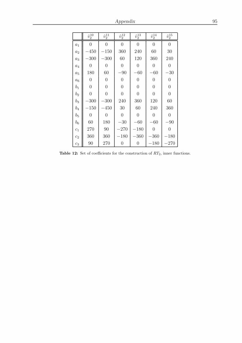
Appendix 95
v102 v112 v122 v132 v142 v152
a1 0 0 0 0 0 0
a2 −450 −150 360 240 60 30
a3 −300 −300 60 120 360 240
a4 0 0 0 0 0 0
a5 180 60 −90 −60 −60 −30
a6 0 0 0 0 0 0
b1 0 0 0 0 0 0
b2 0 0 0 0 0 0
b3 −300 −300 240 360 120 60
b4 −150 −450 30 60 240 360
b5 0 0 0 0 0 0
b6 60 180 −30 −60 −60 −90
c1 270 90 −270 −180 0 0
c2 360 360 −180 −360 −360 −180
c3 90 270 0 0 −180 −270
Table 12: Set of coefficients for the construction of RT2, inner functions.
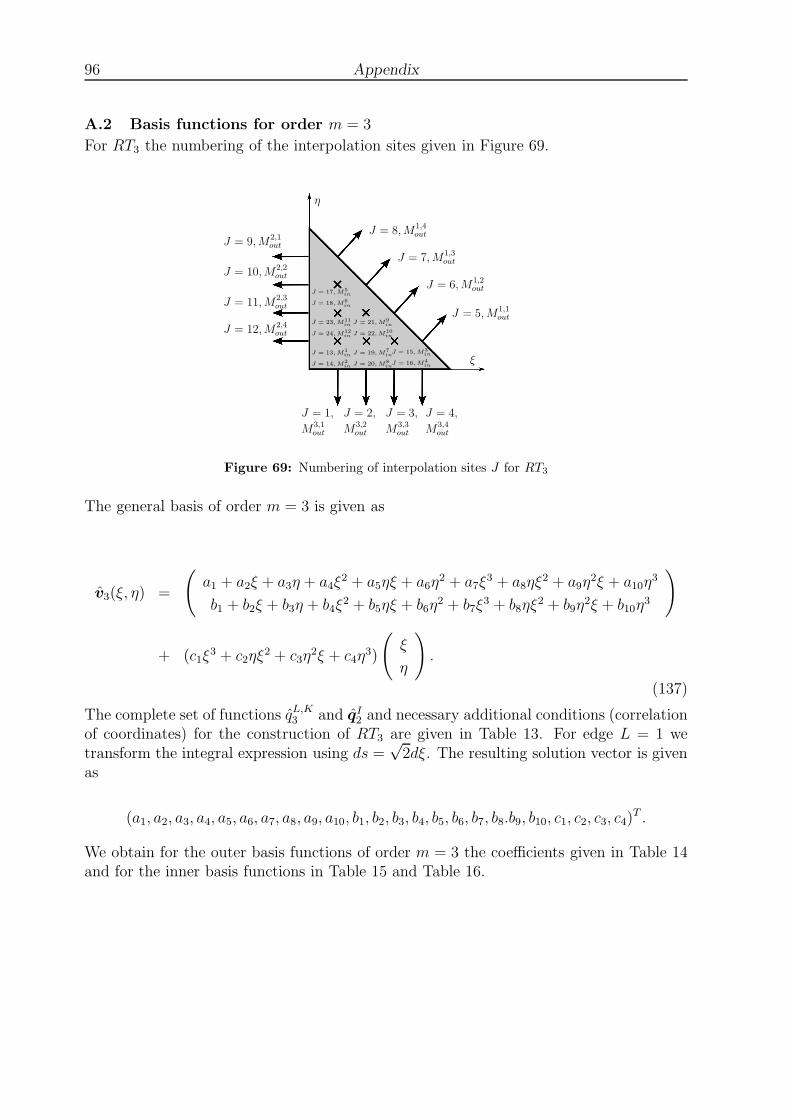
96 Appendix
A.2 Basis functions for order m = 3
For RT3 the numbering of the interpolation sites given in Figure 69.
ξ
η
J = 3,
J = 5,M1,1out
J = 6,M1,2out
J = 7,M1,3out
J = 8,M1,4out
J = 9,M2,1out
J = 10,M2,2out
J = 11,M2,3out
J = 12,M2,4out
J = 13, M1
in
J = 14, M2
in
J = 17, M5
in
J = 18, M6
in
J = 15, M3
in
J = 16, M4
in
J = 1,
M3,1out
J = 2,
M3,2out M3,3
out
J = 4,
M3,4out
J = 23, M11
in
J = 24, M12
in
J = 19,M7
in
J = 20,M8
in
J = 21,M9
in
J = 22,M10
in
Figure 69: Numbering of interpolation sites J for RT3
The general basis of order m = 3 is given as
v3(ξ, η) =
(
a1 + a2ξ + a3η + a4ξ2 + a5ηξ + a6η
2 + a7ξ3 + a8ηξ
2 + a9η2ξ + a10η
3
b1 + b2ξ + b3η + b4ξ2 + b5ηξ + b6η
2 + b7ξ3 + b8ηξ
2 + b9η2ξ + b10η
3
)
+ (c1ξ3 + c2ηξ
2 + c3η2ξ + c4η
3)
(
ξ
η
)
.
(137)
The complete set of functions qL,K3 and qI2 and necessary additional conditions (correlation
of coordinates) for the construction of RT3 are given in Table 13. For edge L = 1 wetransform the integral expression using ds =
√2dξ. The resulting solution vector is given
as
(a1, a2, a3, a4, a5, a6, a7, a8, a9, a10, b1, b2, b3, b4, b5, b6, b7, b8.b9, b10, c1, c2, c3, c4)T .
We obtain for the outer basis functions of order m = 3 the coefficients given in Table 14and for the inner basis functions in Table 15 and Table 16.

Appendix 97
L K I qL,K1 / qI0 correlation of coordinates
1 1 - 83
(9ξ3
2− 9ξ2
2+ ξ)
η = 1− ξ
1 2 - 83
(
−27ξ3
2+ 18ξ2 − 9ξ
2
)
η = 1− ξ
1 3 - 83
(27ξ3
2− 45ξ2
2+ 9ξ
)
η = 1− ξ
1 4 - 83
(
−9ξ3
2+ 9ξ2 − 11ξ
2+ 1)
η = 1− ξ
2 1 - 83
(9η3
2− 9η2
2+ η)
ξ = 0
2 2 - 83
(
−27η3
2+ 18η2 − 9η
2
)
ξ = 0
2 3 - 83
(27η3
2− 45η2
2+ 9η
)
ξ = 0
2 4 - 83
(
−9η3
2+ 9η2 − 11η
2+ 1)
ξ = 0
3 1 - 83
(
−9ξ3
2+ 9ξ2 − 11ξ
2+ 1)
η = 0
3 2 - 83
(27ξ3
2− 45ξ2
2+ 9ξ
)
η = 0
3 3 - 83
(
−27ξ3
2+ 18ξ2 − 9ξ
2
)
η = 0
3 4 - 83
(9ξ3
2− 9ξ2
2+ ξ)
η = 0
- - 1 (2η2 + 4ηξ − 3η + 2ξ2 − 3ξ + 1, 0)T -
- - 2 (0, 2η2 + 4ηξ − 3η + 2ξ2 − 3ξ + 1)T -
- - 3 (2ξ2 − ξ, 0)T -
- - 4 (0, 2ξ2 − ξ)T -
- - 5 (2η2 − η, 0)T -
- - 6 (0, 2η2 − η)T -
- - 7 (0,−4ηξ − 4ξ2 + 4ξ)T -
- - 8 (−4ηξ − 4ξ2 + 4ξ, 0)T -
- - 9 (0, 4ηξ)T -
- - 10 (4ηξ, 0)T -
- - 11 (0,−4η2 − 4ηξ + 4η)T -
- - 12 (−4η2 − 4ηξ + 4η, 0)T -
Table 13: Set of functions qL,K3
and qI2and correlation of coordinates for the construction
of RT3.

98 Appendix
v13 v23 v33 v43 v53 v63 v73 v83 v93 v103 v113 v123
a1 0 0 0 0 0 0 0 0 12
−49
1718
−2
a2 5 −379
199
−2 −2 −92
−3 −12
−12
−149
1918
20
a3 0 0 0 0 0 0 0 0 −152
253
−956
15
a4 −30 1003
−643
18 18 30 12 0 0 133
−763
−60
a5 −30 223
143
0 0 21 30 9 9 6 75 −90
a6 0 0 0 0 0 0 0 0 452
−853
2156
−30
a71052
−63 1052
−42 −42 −1543
−353
0 0 79
4349
70
a8 105 −2663
−493
0 0 −112 −98 0 0 −1192
−98 3152
a91052
563
−496
0 0 −352
−56 −632
−632
1403
−7216
105
a10 0 0 0 0 0 0 0 0 −352
38518
−38518
352
b1 −2 1718
−49
12
0 0 0 0 0 0 0 0
b2 15 −956
253
−152
0 0 0 0 0 0 0 0
b3 20 1918
−149
−12
−12
−3 −92
−2 −2 199
−379
5
b4 −30 2156
−853
452
0 0 0 0 0 0 0 0
b5 −90 75 6 9 9 30 21 0 0 143
223
−30
b6 −60 −763
133
0 0 12 30 18 18 −643
1003
−30
b7352
−38518
38518
−352
0 0 0 0 0 0 0 0
b8 105 −7216
1403
−632
−632
−56 −352
0 0 −496
563
1052
b93152
−98 −1192
0 0 −98 −112 0 0 −493
−2663
105
b10 70 4349
79
0 0 −353
−1543
−42 −42 1052
−63 1052
c1 −28 3089
−3089
28 28 2249
289
0 0 −289
−2249
−28
c2 −84 2803
−283
0 0 112 56 0 0 1403
1123
−84
c3 −84 1123
1403
0 0 56 112 0 0 −283
2803
−84
c4 −28 −2249
−289
0 0 289
2249
28 28 −3089
3089
−28
Table 14: Set of coefficients for the construction of RT3, outer functions.

Appendix 99
v133 v143 v153 v163 v173 v183
a1 0 0 0 0 0 0
a2 960 240 288 216 144 72
a3 0 0 0 0 0 0
a4 −4320 −1080 −2304 −1728 −144 −72
a5 −3240 −2160 −216 −432 −1944 −1152
a6 0 0 0 0 0 0
a7 6048 1512 4704 3528 0 0
a8 9072 6048 1512 3024 2016 1008
a9 3024 4536 0 0 4536 3528
a10 0 0 0 0 0 0
b1 0 0 0 0 0 0
b2 0 0 0 0 0 0
b3 240 960 72 144 216 288
b4 0 0 0 0 0 0
b5 −2160 −3240 −1152 −1944 −432 −216
b6 −1080 −4320 −72 −144 −1728 −2304
b7 0 0 0 0 0 0
b8 4536 3024 3528 4536 0 0
b9 6048 9072 1008 2016 3024 1512
b10 1512 6048 0 0 3528 4704
c1 −2688 −672 −2688 −2016 0 0
c2 −6048 −4032 −2016 −4032 0 0
c3 −4032 −6048 0 0 −4032 −2016
c4 −672 −2688 0 0 −2016 −2688
Table 15: Set of coefficients for the construction of RT3, inner functions, v13
3up to v18
3.

100 Appendix
v193 v203 v213 v223 v233 v243
a1 0 0 0 0 0 0
a2 −48 −66 216 144 6 −12
a3 0 0 0 0 0 0
a4 720 486 −1098 −774 −468 −72
a5 −216 216 −1332 −1044 1188 360
a6 0 0 0 0 0 0
a7 −1344 −756 1554 1134 1134 252
a8 −756 −2268 4788 4032 −2772 −504
a9 504 378 1638 1638 −1512 −1008
a10 0 0 0 0 0 0
b1 0 0 0 0 0 0
b2 0 0 0 0 0 0
b3 −12 6 144 216 −66 −48
b4 0 0 0 0 0 0
b5 360 1188 −1044 −1332 216 −216
b6 −72 −468 −774 −1098 486 720
b7 0 0 0 0 0 0
b8 −1008 −1512 1638 1638 378 504
b9 −504 −2772 4032 4788 −2268 −756
b10 252 1134 1134 1554 −756 −1344
c1 672 336 −672 −504 −672 −168
c2 1008 2016 −3528 −3024 1512 0
c3 0 1512 −3024 −3528 2016 1008
c4 −168 −672 −504 −672 336 672
Table 16: Set of coefficients for the construction of RT3, inner functions, v19
3up to v24
3.

Appendix 101
A.3 Alternative basis functions for order m = 1
Following the alternative way of construction for m = 1 we obtain the vector-valued basisfunctions (respectively the coefficients) as given in Table 17.
v12 v22 v32 v42 v52 v62 v72 v82
a1 0 0 0 0 1 −2 0 0
a2 2 −1 −1 −1 −1 5 6 3
a3 0 0 0 0 −3 3 0 0
b1 −2 1 0 0 0 0 0 0
b2 3 −3 0 0 0 0 0 0
b3 5 −1 −1 −1 −1 2 3 6
c1 −3 3 3 0 0 −3 −6 −3
c2 −3 0 0 3 3 −3 −3 −6
Table 17: Alternative set of coefficients for the construction of RT1.
A.4 Alternative basis functions for order m = 2
Constructing the basis for order m = 2 using the alternative way, leads to the coefficientsfor the outer degrees of freedom given in Table 18 and for the inner basis functions inTable 19.
v12 v22 v32 v42 v52 v62 v72 v82 v92
a1 0 0 0 0 0 0 −1 3 −3
a2 −10 16 −6 −6 −4 0 0 4 −18
a3 −10 4 0 0 −4 −6 −6 32 −26
a4 0 0 0 0 0 0 −8 16 −8
a5 3 −3 1 1 1 1 1 −7 13
a6 0 0 0 0 0 0 6 −16 10
b1 −3 3 −1 0 0 0 0 0 0
b2 −8 16 −8 0 0 0 0 0 0
b3 −26 32 −6 −6 −4 0 0 4 −10
b4 −18 4 0 0 −4 −6 −6 16 −10
b5 10 −16 6 0 0 0 0 0 0
b6 13 −7 1 1 1 1 1 −3 3
c1 8 −16 8 8 0 0 0 0 8
c2 16 −16 0 0 16 0 0 −16 16
c3 8 0 0 0 0 8 8 −16 8
Table 18: Alternative set of coefficients for the construction of RT2, outer functions.

102 Appendix
v102 v112 v122 v132 v142 v152a1 0 0 0 0 0 0a2 −84 −28 60 40 16 8a3 −60 −52 8 16 72 44a4 0 0 0 0 0 0a5 36 12 −12 −8 −16 −8a6 0 0 0 0 0 0b1 0 0 0 0 0 0b2 0 0 0 0 0 0b3 −52 −60 44 72 16 8b4 −28 −84 8 16 40 60b5 0 0 0 0 0 0b6 12 36 −8 −16 −8 −12c1 48 16 −48 −32 0 0c2 64 64 −32 −64 −64 −32c3 16 48 0 0 −32 −48
Table 19: Alternative set of coefficients for the construction of RT2, inner functions.
A.5 Alternative basis functions for order m = 3
The alternative coefficients of the basis functions for order m = 3 for the outer degrees offreedom are given in Table 20, for the inner basis functions in Table 21 and Table 22.
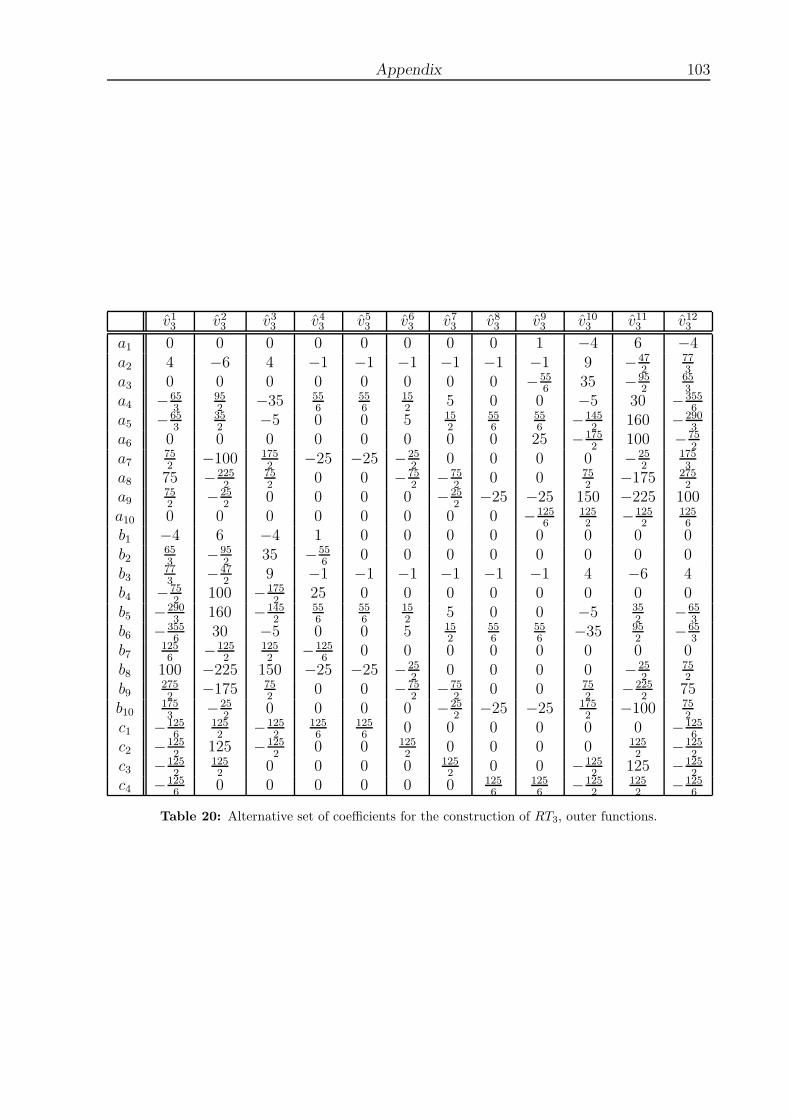
Appendix 103
v13 v23 v33 v43 v53 v63 v73 v83 v93 v103 v113 v123a1 0 0 0 0 0 0 0 0 1 −4 6 −4a2 4 −6 4 −1 −1 −1 −1 −1 −1 9 −47
2773
a3 0 0 0 0 0 0 0 0 −556
35 −952
653
a4 −653
952
−35 556
556
152
5 0 0 −5 30 −3556
a5 −653
352
−5 0 0 5 152
556
556
−1452
160 −2903
a6 0 0 0 0 0 0 0 0 25 −1752
100 −752
a7752
−100 1752
−25 −25 −252
0 0 0 0 −252
1753
a8 75 −2252
752
0 0 −752
−752
0 0 752
−175 2752
a9752
−252
0 0 0 0 −252
−25 −25 150 −225 100a10 0 0 0 0 0 0 0 0 −125
61252
−1252
1256
b1 −4 6 −4 1 0 0 0 0 0 0 0 0b2
653
−952
35 −556
0 0 0 0 0 0 0 0b3
773
−472
9 −1 −1 −1 −1 −1 −1 4 −6 4b4 −75
2100 −175
225 0 0 0 0 0 0 0 0
b5 −2903
160 −1452
556
556
152
5 0 0 −5 352
−653
b6 −3556
30 −5 0 0 5 152
556
556
−35 952
−653
b71256
−1252
1252
−1256
0 0 0 0 0 0 0 0b8 100 −225 150 −25 −25 −25
20 0 0 0 −25
2752
b92752
−175 752
0 0 −752
−752
0 0 752
−2252
75b10
1753
−252
0 0 0 0 −252
−25 −25 1752
−100 752
c1 −1256
1252
−1252
1256
1256
0 0 0 0 0 0 −1256
c2 −1252
125 −1252
0 0 1252
0 0 0 0 1252
−1252
c3 −1252
1252
0 0 0 0 1252
0 0 −1252
125 −1252
c4 −1256
0 0 0 0 0 0 1256
1256
−1252
1252
−1256
Table 20: Alternative set of coefficients for the construction of RT3, outer functions.

104 Appendix
v133 v143 v153 v163 v173 v183
a1 0 0 0 0 0 0
a210003
2503
5009
1253
2503
1253
a3 0 0 0 0 0 0
a4 −117509
−587518
−42509
−21256
−2503
−1253
a5 −95009
−1037518
−1253
−2503
−20003
−662518
a6 0 0 0 0 0 0
a750003
12503
100009
25003
0 0
a815625
631252
6252
625 625 6252
a918752
68756
0 0 81256
18752
a10 0 0 0 0 0 0
b1 0 0 0 0 0 0
b2 0 0 0 0 0 0
b32503
10003
1253
2503
1253
5009
b4 0 0 0 0 0 0
b5 −1037518
−95009
−662518
−20003
−2503
−1253
b6 −587518
−117509
−1253
−2503
−21256
−42509
b7 0 0 0 0 0 0
b868756
18752
18752
81256
0 0
b931252
156256
6252
625 625 6252
b1012503
50003
0 0 25003
100009
c1 −62509
−312518
−62509
−31256
0 0
c2 −31252
−31253
−31256
−31253
0 0
c3 −31253
−31252
0 0 −31253
−31256
c4 −312518
−62509
0 0 −31256
−62509
Table 21: Alternative set of coefficients for the construction of RT3, inner functions, v133
up to v183 .

Appendix 105
v193 v203 v213 v223 v233 v243
a1 0 0 0 0 0 0
a2 −1254
−1258
37532
12516
−3758
−1258
a3 0 0 0 0 0 0
a4362516
362532
−112516
−3758
337532
112532
a587516
212532
−212532
−162532
987532
412532
a6 0 0 0 0 0 0
a7 −31258
−312516
187532
62516
−187532
−62532
a8 −1062532
−1312532
31258
937532
−1937532
−18758
a9 −62532
−187532
62516
187532
−31258
−937532
a10 0 0 0 0 0 0
b1 0 0 0 0 0 0
b2 0 0 0 0 0 0
b3 −1258
−3758
12516
37532
−1258
−1254
b4 0 0 0 0 0 0
b5412532
987532
−162532
−212532
212532
87516
b6112532
337532
−3758
−112516
362532
362516
b7 0 0 0 0 0 0
b8 −937532
−31258
187532
62516
−187532
−62532
b9 −18758
−1937532
937532
31258
−1312532
−1062532
b10 −62532
−187532
62516
187532
−312516
−31258
c1312516
312532
0 0 0 0
c2937532
31258
−937532
−312516
937532
312532
c3312532
937532
−312516
−937532
31258
937532
c4 0 0 0 0 312532
312516
Table 22: Alternative set of coefficients for the construction of RT3, inner functions, v193
up to v243 .
A.6 Further courses of the reaction forces for the Cook’s Membrane example
In the following further results of Chapter 5.3 are shown. In Figure the course of thereaction forces at the left boundary of the Cook’s Membrane problem for P1P2 and RT1P2
are depicted for two additional meshes under consideration of different weights ωi. For thestandard and the mixed Galerkin element the additional computations are shown in Figure71. Finally, in Figure 72 the evaluation of the reaction forces for higher order least-squareselements are depicted under consideration of the weightings ω1 = 1, ω2 = ω3 = 1/µ.
A.7 Shear stress distribution for the example of the quartered plate.
Figure 73 show the distribution of the shear stresses σ12 and σ21 over the domain of thequartered plate for two different fine meshes.

106 Appendix
0.0
11.0
22.0
33.0
44.0
-0.6 -0.4 -0.2 0.0 0.2
x2
σn
P1P2, (1, 1/µ, 1/µ), neq = 11164
σ11σ21 0.0
11.0
22.0
33.0
44.0
-0.6 -0.4 -0.2 0.0 0.2
x2
σn
P1P2, (100, 1/µ, 0), neq = 11164
σ11σ21
0.0
11.0
22.0
33.0
44.0
-0.6 -0.4 -0.2 0.0 0.2
x2
σn
P1P2, (1, 1/µ, 1/µ), neq = 19684
σ11σ21 0.0
11.0
22.0
33.0
44.0
-0.6 -0.4 -0.2 0.0 0.2
x2
σn
P1P2, (100, 1/µ, 0), neq = 19684
σ11σ21
0.0
11.0
22.0
33.0
44.0
-0.6 -0.4 -0.2 0.0 0.2
x2
σn
RT1P2, (1, 1/µ, 1/µ), neq = 11200
σ11σ21 0.0
11.0
22.0
33.0
44.0
-0.6 -0.4 -0.2 0.0 0.2
x2
σn
RT1P2, (100, 1/µ, 0), neq = 11200
σ11σ21
0.0
11.0
22.0
33.0
44.0
-0.6 -0.4 -0.2 0.0 0.2
x2
σn
RT1P2, (1, 1/µ, 1/µ), neq = 25200
σ11σ21 0.0
11.0
22.0
33.0
44.0
-0.6 -0.4 -0.2 0.0 0.2
x2
σn
RT1P2, (100, 1/µ, 0), neq = 25200
σ11σ21
Figure 70: Course of the support reactions for P1P2 and RT1P2 under consideration ofdifferent system sizes neq and different weights ωi .

Appendix 107
0.0
11.0
22.0
33.0
44.0
-0.6 -0.4 -0.2 0.0 0.2
x2
σn
T2, neq = 33024
σ11σ21 0.0
11.0
22.0
33.0
44.0
-0.6 -0.4 -0.2 0.0 0.2
x2
σn
T2P0, neq = 33024
σ11σ21
0.0
11.0
22.0
33.0
44.0
-0.6 -0.4 -0.2 0.0 0.2
x2
σn
T2, neq = 8320
σ11σ21 0.0
11.0
22.0
33.0
44.0
-0.6 -0.4 -0.2 0.0 0.2
x2
σn
T2P0, neq = 8320
σ11σ21
Figure 71: Course of the support reactions for T2 and T2P0 under consideration of differentsystem sizes neq .

108 Appendix
0.0
11.0
22.0
33.0
44.0
-0.6 -0.4 -0.2 0.0 0.2
x2
σn
RT2P3, (1, 1/µ, 1/µ), neq = 2160
σ11σ21 0.0
11.0
22.0
33.0
44.0
-0.6 -0.4 -0.2 0.0 0.2
x2
σn
RT2P3, (1, 1/µ, 1/µ), neq = 8640
σ11σ21
0.0
11.0
22.0
33.0
44.0
-0.6 -0.4 -0.2 0.0 0.2
x2
σn
RT2P3, (1, 1/µ, 1/µ), neq = 19440
σ11σ21 0.0
11.0
22.0
33.0
44.0
-0.6 -0.4 -0.2 0.0 0.2
x2
σn
RT2P3, (1, 1/µ, 1/µ), neq = 34560
σ11σ21
0.0
11.0
22.0
33.0
44.0
-0.6 -0.4 -0.2 0.0 0.2
x2
σn
RT3P4, (1, 1/µ, 1/µ), neq = 1664
σ11σ21 0.0
11.0
22.0
33.0
44.0
-0.6 -0.4 -0.2 0.0 0.2
x2
σn
RT3P4, (1, 1/µ, 1/µ), neq = 6656
σ11σ21
0.0
11.0
22.0
33.0
44.0
-0.6 -0.4 -0.2 0.0 0.2
x2
σn
RT3P4, (1, 1/µ, 1/µ), neq = 14976
σ11σ21 0.0
11.0
22.0
33.0
44.0
-0.6 -0.4 -0.2 0.0 0.2
x2
σn
RT3P4, (1, 1/µ, 1/µ), neq = 26624
σ11σ21
Figure 72: Course of the support reactions for RT2P3 and RT3P4 under consideration ofdifferent system sizes neq .

Appendix 109
RT1P2 P1P2 T2P0
RT1P2 P1P2 T2P0
σ12
RT1P2 P1P2 T2P0
RT1P2 P1P2 T2P0
σ21
Figure 73: Distribution of the σ12 stresses (upper six plots) and σ21 stresses (lower sixplots) for the quartered plate meshed with 20x20 elements (above) and 80x80 elements(below).


LIST OF FIGURES 111
List of Figures
1 Mappings of the infinitesimal line, area and volume elements, F : dX 7→dx,Cof F : dA 7→ da and detF : dV 7→ dv. . . . . . . . . . . . . . . . . 8
2 Body with cutting plane and internal stress vectors T and t. . . . . . . . . 11
3 Pascal’s triangle for the monomials for two-dimensional interpolation func-tions. . . . . . . . . . . . . . . . . . . . . . . . . . . . . . . . . . . . . . . . 16
4 Numbering of edges eL and their associated normals nL. . . . . . . . . . . 17
5 Piola transformation. . . . . . . . . . . . . . . . . . . . . . . . . . . . . . . 19
6 Numbering of interpolation sites J for RT1. . . . . . . . . . . . . . . . . . . 20
7 Plot of the Raviart-Thomas functions ΨJ2 over the edge e3 on a unit trian-
gular domain . . . . . . . . . . . . . . . . . . . . . . . . . . . . . . . . . . 23
8 Plot of the alternative Raviart-Thomas functions ΨJ2 over the edge e3 on a
unit triangular domain . . . . . . . . . . . . . . . . . . . . . . . . . . . . . 23
9 Plot of the basis functions v32 , v
62, v
72 and v14
2 . . . . . . . . . . . . . . . . . . 24
10 Stress-strain- curve (λ = 0, µ = 1), 1D. . . . . . . . . . . . . . . . . . . . . 30
11 Mixed reference element (Ωe) in 1D. . . . . . . . . . . . . . . . . . . . . . . 31
12 Setup boundary value problem in 1D. . . . . . . . . . . . . . . . . . . . . . 34
13 Solution for the displacements u, Mathematica vs LSM, 1D. . . . . . . . . 36
14 Arrangement of element nodes J for RT . . . . . . . . . . . . . . . . . . . . 38
15 Arrangement of element nodes I for P . . . . . . . . . . . . . . . . . . . . . 39
16 Stress state of an infinitesimal part. . . . . . . . . . . . . . . . . . . . . . . 42
17 Geometry of the uniaxial tension test. . . . . . . . . . . . . . . . . . . . . . 42
18 Adding further additional nodes using the ”SMSAdditionalNodes” com-mand exemplary for RT1P2. . . . . . . . . . . . . . . . . . . . . . . . . . . 44
19 Computation of the kinematic quantities. . . . . . . . . . . . . . . . . . . . 45
20 Two elements sharing one edge, orientation of the normal for the localtraction vector. . . . . . . . . . . . . . . . . . . . . . . . . . . . . . . . . . 45
21 Definition of the free energy function. . . . . . . . . . . . . . . . . . . . . . 46
22 Automatic differentiation of the free energy with respect to the deformationgradient F . . . . . . . . . . . . . . . . . . . . . . . . . . . . . . . . . . . . 46
23 Applying automatic differentiation and filling right-hand-side and stiffnessmatrix. . . . . . . . . . . . . . . . . . . . . . . . . . . . . . . . . . . . . . . 46
24 Geometry of the cantilever beam. . . . . . . . . . . . . . . . . . . . . . . . 48
25 Displacement convergence for u2 of the upper right node (10,1) over numberof equations (neq) of the final system of equations for RTmPk . . . . . . . . 49
26 Displacement convergence for u2 of the upper right node (10,1) over numberof equations (neq) of the final system of equations for PmPk . . . . . . . . . 50

112 LIST OF FIGURES
27 Displacement convergence for u2 of the upper right node (10,1) over numberof equations (neq) of the final system of equations for best tested combi-nations RTmPk and PmPk. . . . . . . . . . . . . . . . . . . . . . . . . . . . 50
28 Plot of u2-displacement of the upper right node (lower) for RT1P2 consid-ering different weights ω3. . . . . . . . . . . . . . . . . . . . . . . . . . . . 51
29 Plot of the squared L2(B) norms of the individual residuals Ri and plot ofthe functional error for different weights ωi for RT1P2 . . . . . . . . . . . . 52
30 Geometry and mesh (20×20 elements) of the Cook’s membrane. . . . . . . 53
31 Displacement convergence of the upper right node with the coordinates(48,60) for different elements . . . . . . . . . . . . . . . . . . . . . . . . . . 54
32 Distribution of the σ11 component of the Cauchy stresses for different ele-ments and distribution of the functional error for RT1P2 (lower left). . . . . 55
33 Resulting horizontal and vertical reaction forces for different elements . . . 56
34 Course of the support reactions for the least-squares elements of type P1P2
and RT1P2 under consideration of different system sizes neq and differentweights ωi . . . . . . . . . . . . . . . . . . . . . . . . . . . . . . . . . . . . 57
35 Course of the support reactions for the Galerkin elements T2 and T2P0
under consideration of different system sizes neq . . . . . . . . . . . . . . . 58
36 Geometry of the quartered plate (left) and typical mesh on deformed con-figuration (right), RT1P2, 20x20 elements per side. . . . . . . . . . . . . . . 59
37 Distribution of the P22 stresses for the quartered plate meshed with 20x20(above) and 80x80 (below) elements. . . . . . . . . . . . . . . . . . . . . . 59
38 Distribution of the σ22 stresses for the quartered plate meshed with 20x20(above) and 80x80 (below) elements. . . . . . . . . . . . . . . . . . . . . . 60
39 Geometry of the compression test and typical mesh in the deformed con-figuration for RT2P3. . . . . . . . . . . . . . . . . . . . . . . . . . . . . . . 61
40 Plot of detF over the deformed shape of the compression test for the mixedleast-squares element RT2P3 (left) and the mixed Galerkin element T2P0
(right). . . . . . . . . . . . . . . . . . . . . . . . . . . . . . . . . . . . . . . 62
41 Geometry of the clamped plate. . . . . . . . . . . . . . . . . . . . . . . . . 62
42 Displacement convergence for u3 of node (10, 10, 1) over the number ofequations (neq) of the final system of equations for RT0P2 and T2 . . . . . 63
43 Stress component P11 on the deformed shape of the clamped plate underbodyforce for T2 (left) and RT0P2 (right). . . . . . . . . . . . . . . . . . . . 63
44 Geometry of the cantilever beam. . . . . . . . . . . . . . . . . . . . . . . . 64
45 Displacement of the upper right node of the cantilever beam over differentangles γ denoting the prefered direction . . . . . . . . . . . . . . . . . . . . 64
46 Geometry of the cantilever beam. . . . . . . . . . . . . . . . . . . . . . . . 67
47 Log-log plot of Fh (left) and u2-displacement of the upper right node (right)for RT0P1. . . . . . . . . . . . . . . . . . . . . . . . . . . . . . . . . . . . . 68

LIST OF FIGURES 113
48 Log-log plot of Fh (left) and u2-displacement of the upper right node (right)for RT1P2. . . . . . . . . . . . . . . . . . . . . . . . . . . . . . . . . . . . . 69
49 Log-log plot of Fh (left) and u2-displacement of the upper right node (right)for RT2P3. . . . . . . . . . . . . . . . . . . . . . . . . . . . . . . . . . . . . 69
50 Log-log plot of Fh (left) and u2-displacement of the upper right node (right)for RT3P4. . . . . . . . . . . . . . . . . . . . . . . . . . . . . . . . . . . . . 70
51 Log-log plot of |u− uh| (left) and u2-displacement of the upper right node(right) for T2. . . . . . . . . . . . . . . . . . . . . . . . . . . . . . . . . . . 70
52 Exemplary regular mesh refinement for the Cook’s Membrane problem with4, 8, 16 and 32 elements per edge. . . . . . . . . . . . . . . . . . . . . . . . 73
53 Exemplary adaptive mesh refinement for the Cook’s Membrane problem. . 74
54 Basis nodes and new nodes for three respectiveley seven additional nodesrefinement strategy. . . . . . . . . . . . . . . . . . . . . . . . . . . . . . . . 76
55 Geometry and boundary conditions of the plate with a hole. . . . . . . . . 76
56 Initial meshes with nearly same system size. . . . . . . . . . . . . . . . . . 77
57 Refinement stages for regular refinemnt (rr, left), error percent marking(arD, middle) and element percent marking (arE, right). . . . . . . . . . . 78
58 Regular and error percent marking strategy: Log-log plot of |F −Fh| (left)and u2-displacement of the circle node (x1 = 0, x2 = 1) (right). . . . . . . . 79
59 Regular and element percent marking strategy: Log-log plot of |F − Fh|(left) and u2-displacement of the circle node (x1 = 0, x2 = 1) (right). . . . 80
60 Error percent and element percent marking strategy: Log-log plot of |F −Fh| (left) and u2-displacement of the circle node (x1 = 0, x2 = 1) (right). . 80
61 Von Mises stresses over the deformed shape for several refinement levels. . 81
62 Load-deflection curve with bifurcation point at γcrit. . . . . . . . . . . . . . 83
63 First and third Euler case. . . . . . . . . . . . . . . . . . . . . . . . . . . . 84
64 Results of stability analysis for T2 (left,red) and RT1P2 (right,blue) forEuler case 1 (above) and for Euler case 3 (below) . . . . . . . . . . . . . . 85
65 Incompressible blocks for stability analysis, problem 2 in Auricchio et al.[2010] (left) and problem 1 in Auricchio et al. [2013] (right). . . . . . . . . 86
66 Result of stability analysis for the standard Galerkin element T2 (left) andthe least-squares element RT1P2 (right) for different number of equations(stated in the legend) for problem 2 in Auricchio et al. [2010]. . . . . . . . 87
67 Result of stability analysis for the standard Galerkin element T2 (left) andthe least-squares elements RT1P2 and RT2P3 (right) for problem 1 in Au-ricchio et al. [2013] . . . . . . . . . . . . . . . . . . . . . . . . . . . . . . . 88
68 Numbering of interpolation sites J for RT2 . . . . . . . . . . . . . . . . . . 93
69 Numbering of interpolation sites J for RT3 . . . . . . . . . . . . . . . . . . 96
70 Course of the support reactions for P1P2 and RT1P2 under considerationof different system sizes neq and different weights ωi . . . . . . . . . . . . . 106

114 LIST OF FIGURES
71 Course of the support reactions for T2 and T2P0 under consideration ofdifferent system sizes neq . . . . . . . . . . . . . . . . . . . . . . . . . . . . 107
72 Course of the support reactions for RT2P3 and RT3P4 under considerationof different system sizes neq . . . . . . . . . . . . . . . . . . . . . . . . . . 108
73 Distribution of the σ12 stresses (upper six plots) and σ21 stresses (lowersix plots) for the quartered plate meshed with 20x20 elements (above) and80x80 elements (below). . . . . . . . . . . . . . . . . . . . . . . . . . . . . 109

LIST OF TABLES 115
List of Tables
1 Raviart-Thomas setups (m = 0, 1, 2, 3) in two dimensions. . . . . . . . . . . 17
2 Set of functions qL,K1 and qI0 and correlation of coordinates for the con-
struction of RT1. . . . . . . . . . . . . . . . . . . . . . . . . . . . . . . . . 21
3 Set of coefficients for the construction of RT1. . . . . . . . . . . . . . . . . 22
4 Number of element nodes (nen) and number of degrees of freedom perelement (edof) for the different two-dimensional element types under con-sideration. . . . . . . . . . . . . . . . . . . . . . . . . . . . . . . . . . . . . 38
5 Material parameters used for the investigation of locking. . . . . . . . . . . 68
6 Convergence rates of the elements used for different values of λ. . . . . . . 71
7 Minimum and maximum values of detF for different values of λ using anRT1P2 element with neq = 28000. . . . . . . . . . . . . . . . . . . . . . . . 71
8 Number of equtions of the initial meshes for the different element types. . . 77
9 Convergence rates of the elements used for regular and adaptive refinement. 79
10 Set of functions qL,K2 and qI1 and correlation of coordinates for the con-
struction of RT3. . . . . . . . . . . . . . . . . . . . . . . . . . . . . . . . . 94
11 Set of coefficients for the construction of RT2, outer functions. . . . . . . . 94
12 Set of coefficients for the construction of RT2, inner functions. . . . . . . . 95
13 Set of functions qL,K3 and qI2 and correlation of coordinates for the con-
struction of RT3. . . . . . . . . . . . . . . . . . . . . . . . . . . . . . . . . 97
14 Set of coefficients for the construction of RT3, outer functions. . . . . . . . 98
15 Set of coefficients for the construction of RT3, inner functions, v133 up to v183 . 99
16 Set of coefficients for the construction of RT3, inner functions, v193 up to v243 .100
17 Alternative set of coefficients for the construction of RT1. . . . . . . . . . . 101
18 Alternative set of coefficients for the construction of RT2, outer functions. . 101
19 Alternative set of coefficients for the construction of RT2, inner functions. . 102
20 Alternative set of coefficients for the construction of RT3, outer functions. . 103
21 Alternative set of coefficients for the construction of RT3, inner functions,v133 up to v183 . . . . . . . . . . . . . . . . . . . . . . . . . . . . . . . . . . . 104
22 Alternative set of coefficients for the construction of RT3, inner functions,v193 up to v243 . . . . . . . . . . . . . . . . . . . . . . . . . . . . . . . . . . . 105


References 117
References
AceDoc. https://wiki.uni-due.de/acedoc/. Internal wiki, Institute of Mechanics, Depart-ment of Civil Engineering, 2016.
J. Ahrens, B. Geveci, and C. Law. ParaView: An End-User Tool for Large Data Vi-sualization, Visualization Handbook. Elsevier, version 10.1 edition, 2005. Champaign,Illinois.
J.H. Argyris. Energy theorems and structural analysis: Part ii. Aircraft Engineering andAerospace Technology, 27(2):42–58, 1955.
J.H. Argyris and D.E.S. Kelsey. Energy theorems and structural analysis: Part i. AircraftEngineering and Aerospace Technology, 26:410–422, 1954.
F. Auricchio, L. Beirao da Veiga, C. Lovadina, and A. Reali. A stability study of somemixed finite elements for large deformation elasticity problems. Computer Methods inApplied Mechanics and Engineering, 194:1075–1092, 2005.
F. Auricchio, L. Beirao da Veiga, C. Lovadina, and A. Reali. The importance of the exactsatisfaction of the incompressibility constraint in nonlinear elasticity: Mixed FEMsversus NURBS-based approximations. Computer Methods in Applied Mechanics andEngineering, 199:314–323, 2010.
F. Auricchio, L. Beirao da Veiga, C. Lovadina, A. Reali, R.L. Taylor, and P. Wrigger.Approximation of incompressible large deformation elastic problems: some unresolvedissues. Computational Mechanics, 52:1153–1167, 2013.
A.K. Aziz, R.B. Kellogg, and A.B. Stephens. Least squares methods for elliptic systems.Mathematics of computation, 44(169):53–70, 1985.
I. Babuska. The finite element method with lagrangian multipliers. Numerische Mathe-matik, 20(3):179–192, 1973.
I. Babuska and W.C. Rheinboldt. A unified least-squares formulation for fluid-structureinteraction problems. SIAM Journal on Mathematical Analysis, 15(4):736–754, 1978.
I. Babuska and M. Suri. Locking effects in the finite element approximation of elasticityproblems. Numerische Mathematik, 62(1):439–463, 1992.
D. Balzani. Polyconvex anisotropic energies and modeling of damage applied to arterialwalls. PhD thesis, University Duisburg-Essen, Verlag Gluckauf Essen, 2006.
D. Balzani, P. Neff, J. Schroder, and G.A. Holzapfel. A polyconvex framework for soft bi-ological tissues. adjustment to experimental data. International Journal for NumericalMethods in Engineering, 43(20):6052–6070, 2006.
K.-J. Bathe. Finite Element Procedures. Prentice Hall, 1995.
K.-J. Bathe. The inf–sup condition and its evaluation for mixed finite element methods.Computers and Structures, 79(2):243–252, 2001.
B.C. Bell and K.S. Surana. A space-time coupled p-version least-squares finite elementformulation for unsteady fluid dynamics problems. International Journal for NumericalMethods in Engineering, 37:3545–3569, 1994.

118 References
T. Belytschko, W.K. Liu, and B. Moran. Nonlinear Finite Elements for Continua andStructures. John Wiley and Sons, Chichester, 2000.
M. Berndt, T.A. Manteuffel, and S.F. McCormick. Local error estimates and adaptiverefinement for first-order system least squares. Electronic Transactions on NumericalAnalysis, 6:35–43, 1997.
F. Bertrand, S. Munzenmaier, and G. Starke. First-order system least squares on curvedboundaries. SIAM Journal on Scientific Computing, 52:880–894, 2014.
M. Bischoff, W.A. Wall, and E. Ramm. Stabilized enhanced assumed strain elements forlarge strain analysis without artificial kinematic modes. Proc. European Conference onComputational Mechanics, 1999.
P.B. Bochev. Least-Squares Finite Element Methods for the Stokes and Navier-Stokesequations. Phd thesis, Virginia Polytechnic Institute and State University, Blacksburg,Virginia, 1994.
P.B. Bochev. Negative norm least-squares methods for the velocity-vorticity-pressureNavier-Stokes equations. Numerical Methods for Partial Differential Equations, 15:237–256, 1999.
P.B. Bochev and M.D. Gunzburger. Analysis of least squares finite element methods forthe Stokes equations. Mathematics of Computation, 63:479–506, 1994.
P.B. Bochev and M.D. Gunzburger. Least-squares methods for the velocity-pressure-stress formulation of the Stokes equations. Computer Methods in Applied Mechanicsand Engineering, 126:267–287, 1995.
P.B. Bochev and M.D. Gunzburger. Least-Squares Finite Element Methods. Springer-Verlag, New York, 1st edition, 2009.
P.B. Bochev, Z. Cai, T.A. Manteuffel, and S.F. McCormick. Analysis of velocity-flux least-squares methods for the Navier-Stokes equations, part I. SIAM Journal on NumericalAnalysis, 35:990–1009, 1998.
P.B. Bochev, T. Manteuffel, and S. McCormick. Analysis of velocity-flux least squaresmethods for the Navier-Stokes equations, part II. SIAM Journal on Numerical Analysis,36:1125–1144, 1999.
D. Boffi, F. Brezzi, and M. Fortin. Mixed Finite Element Methods and Applications.Springer, Heidelberg, 2013.
D. Braess. Finite Elemente. Springer-Verlag, Berlin, 2nd edition, 1997.
F. Brezzi. On the existence, uniqueness and approximation of saddle-point problems aris-ing from lagrangian multipliers. Revue francaise d’automatique, informatique, rechercheoperationnelle. Analyse numerique, 8(2):129–151, 1974.
F. Brezzi, J. Douglas, and L.D. Martini. Two families of mixed finite elements for secondorder elliptic problems. Numerische Mathematik, 47:217–325, 1985.
Z. Cai and G. Starke. First-order system least squares for the stress-displacement formu-lation: Linear elasticity. SIAM Journal on Numerical Analysis, 41:715–730, 2003.
Z. Cai and G. Starke. Least-squares methods for linear elasticity. SIAM Journal onNumerical Analysis, 42:826–842, 2004.

References 119
Z. Cai, R. Lazarov, T.A. Manteuffel, and S.F. McCormick. First-order system least squaresfor second-order partial differential equations: Part I. SIAM Journal on NumericalAnalysis, 31:1785–1799, 1994.
Z. Cai, T.A. Manteuffel, and S.F. McCormick. First-order system least squares forvelocity-vorticity-pressure form of the Stokes equations, with application to linear elas-ticity. Electronic Transactions on Numerical Analysis, 3:150–159, 1995.
Z. Cai, T.A. Manteuffel, and S.F. McCormick. First-order system least squares for theStokes equation, with application to linear elasticity. SIAM Journal on NumericalAnalysis, 34:1727–1741, 1997.
Z. Cai, T.A. Manteuffel, S.F. McCormick, and S.V. Parter. First-order system leastsquares (FOSLS) for planar linear elasticity: Pure traction problem. SIAM Journal onNumerical Analysis, 35:320–335, 1998.
Z. Cai, C.-O. Lee, T.A. Manteuffel, and S.F. McCormick. First-order system least squaresfor linear elasticity: Numerical results. SIAM Journal on Scientific Computing, 21:1706–1727, 2000a.
Z. Cai, C.-O. Lee, T.A. Manteuffel, and S.F. McCormick. First-order system least squaresfor the Stokes and linear elasticity equations: Further results. SIAM Journal on Scien-tific Computing, 21:1728–1739, 2000b.
Z. Cai, J. Korsawe, and G. Starke. An adaptive least squares mixed finite element methodfor the stress-displacement formulation of linear elasticity. Numerical Methods for Par-tial Differential Equations, 21:132–148, 2005.
C. Chang and B.-N. Jiang. An error analysis of least-squares finite element method ofvelocity-pressure-vorticity formulation for the Stokes problem. Computer Methods inApplied Mechanics and Engineering, 84:247–255, 1990.
C. Chang, S.Y Yang, and C.H. Hsu. A least-squares finite element method for incompress-ible flow in stress-velocity-pressure version. Computer Methods in Applied Mechanicsand Engineering, 128:1–9, 1995.
P.G. Ciarlet. Handbook of Numerical Analysis, vol II: Finite Element Methods, Part 1.Elsevier Science Ltd, 1991.
P.G. Ciarlet and G. Geymonat. Sur les lois de comportement en elasticite non-lineairecompressible. CR Acad. Sci. Paris Ser. II, 295:423–426, 1982.
R.W. Clough. The finite element method in plane stress analysis. 1960.
E.A. de Souza Neto, F.M. Andrade Pires, and D.R.J. Owen. Design of simple low orderfinite elements for large strain analysis of nearly incompressible solids. InternationalJournal of Solids and Structures, 33:3277–3296, 1996.
E.A. de Souza Neto, F.M. Andrade Pires, and D.R.J. Owen. F-bar based linear trianglesand tetrahedra for finite strain analysis of nearly incompressible solids. Part I: formu-lation and benchmarking. International Journal of Solids and Structures, 62:353–383,2005.
B. Delaunay. Sur la sphere vide. Izv. Akad. Nauk SSSR, Otdelenie Matematicheskii iEstestvennyka Nauk, 7(793-800):1–2, 1934.

120 References
X. Ding and T.T.H. Tsang. Large eddy simulation of turbulent flows by a least-squaresfinite element method. International Journal for Numerical Methods in Fluids, 37:297–319, 2001.
X. Ding and T.T.H. Tsang. On first-order formulations of the least-squares finite ele-ment method for incompressible flows. International Journal of Computational FluidDynamics, 17:183–197, 2003.
W.P. Doherty, E.L. Wilson, and R.L. Taylor. Stress analysis of axisymmetric solidsutilizing higher order quadrilateral finite elements, sesm report 69-3, department ofcivil engineering. University of California, Berkeley, 1969.
C.R. Dohrmann, M. W. Heinstein, J. Jung, S. W. Key, and W. R. Witkowski. Node-baseduniform strain elements for three-node triangular and four-node tetrahedral meshes.International Journal for Numerical Methods in Engineering, 47:1549–1568, 2000.
W. Dorfler. A convergent adaptive algorithm for poisson’s equation. SIAM Journal onNumerical Analysis, 33(3):1106–1124, 1996.
A. Duster, S. Hartmann, and E. Rank. p-fem applied to finite isotropic hyperelasticbodies. Computer Methods in Applied Mechanics and Engineering, 192(47):5147–5166,2003.
E.D. Eason. A review of least-squares methods for solving partial differential equations.International Journal for Numerical Methods in Engineering, 10:1021–1046, 1976.
V. Ebbing. Design of Polyconvex Energy Functions for All Anisotropy Classes. PhDthesis, Institut fur Mechanik, Abteilung Bauwissenschaften, Fakultat fur Ingenieurwis-senschaften, Universitat Duisburg-Essen, 2010.
A.C. Eringen. Mechanics of continua. John Wiley & Sons, 1967.
A. Ern and J.-L. Guermond. Theory and practice of finite elements, volume 159. SpringerScience & Business Media, 2013.
V.J. Ervin. Computational bases for RTk and BDMk on triangles. Computers andMathematics with Applications, 64(8):2765–2774, 2012.
L. Euler. Methodus inveniendi lineas curvas maximi minimive proprietate gaudentes sivesolutio problematis isoperimetrici latissimo sensu accepti. Additamentum I : De curviselasticis. Lausannae & Genevae, 1744.
G.J. Fix, M.D. Gunzburger, and R.A. Nicolaides. On finite element methods of the leastsquares type. Computers and Mathematics with Applications, 5:87–98, 1979.
C. Freischlager and K. Schweizerhof. On a systematic development of trilinear three-dimensional solid elements based on Simo’s enhanced strain approach. InternationalJournal of Solids and Structures, 33,No.20-22:2993–3017, 1996.
B.G. Galerkin. Series solution of some problems of elastic equilibrium of rods and plates.Vestn. Inzh. Tekh, 19:897–908, 1915.
M.W. Gee, C.R. Dohrmann, S.W. Key, and W.A. Wall. A uniform nodal strain tetra-hedron with isochoric stabilization. International Journal for Numerical Methods inEngineering, 78:429–443, 2009.

References 121
U. Heisserer, S. Hartmann, A. Duster, and Z. Yosibash. On volumetric locking-free be-haviour of p-version finite elements under finite deformations. Communications innumerical methods in engineering, 24(11):1019–1032, 2008.
G.A. Holzapfel. Nonlinear Solid Mechanics - A Continuum Approach for Engineering.John Wiley and Sons, 2000.
H. Jarausch. On an adaptive grid refining technique for finite element approximations.SIAM journal on scientific and statistical computing, 7(4):1105–1120, 1986.
D. Jespersen. A least-squares decomposition method for solving elliptic equations. Math-ematics of Computation, 31:873–880, 1977.
B.-N. Jiang. A least-squares finite element method for incompressible Navier-Stokes prob-lems. International Journal for Numerical Methods in Fluids, 14:843–859, 1992.
B.-N. Jiang. The Least-Squares Finite Element Method. Springer-Verlag, Berlin, 1998.
B.-N. Jiang. The least-squares finite element method in elasticity. Part ii: Bending of thinplates. International Journal for Numerical Methods in Engineering, 54(10):1459–1475,2002.
B.-N. Jiang and C.L. Chang. Least-squares finite elements for the Stokes problem. Com-puter Methods in Applied Mechanics and Engineering, 78:297–311, 1990.
B.-N. Jiang and J. Wu. The least-squares finite element method in elasticity. Part I: Planestress or strain with drilling degrees of freedom. International Journal for NumericalMethods in Engineering, 53:621–636, 2002.
C. Johnson. Adaptive finite element methods for diffusion and convection problems.Computer Methods in Applied Mechanics and Engineering, 82(1-3):301–322, 1990.
C. Kadapa, W.G. Dettmer, and D. Peric. Nurbs based least-squares finite element meth-ods for fluid and solid mechanics. International Journal for Numerical Methods inEngineering, 101(7):521–539, 2015.
O. Kayser-Herold and H.G. Matthies. Space-time adaptive solution of fluid-structureinteraction problems. In 2nd MIT Conference on Computational Fluid and Solid Me-chanics, Amsterdam, pages 1000–1004, 2003.
O. Kayser-Herold and H.G. Matthies. Least-squares FEM, literature review. Informatik-Bericht 2005-05, TU Braunschweig, Institut fur Wissenschaftliches Rechnen, 2005.
O. Kayser-Herold and H.G. Matthies. A unified least-squares formulation for fluid-structure interaction problems. Computers and Structures, 85:998–1011, 2007.
S.D. Kim, T.A. Manteuffel, and S.F. McCormick. First-order system least squares(FOSLS) for spatial linear elasticity: Pure traction. SIAM Journal on Numerical Anal-ysis, 38:1454–1482, 2000.
O. Klaas, J. Schroder, E. Stein, and C. Miehe. A regularized dual mixed element for planeelasticity implementation and performance of the BDM element. Computer Methods inApplied Mechanics and Engineering, 121:201–209, 1995.
J. Korelc. Automatic generation of finite-element code by simultaneous optimization ofexpressions. Theoretical Computer Science, 187:231–248, 1997.

122 References
J. Korelc. Multi-language and multi-environment generation of nonlinear finite elementcodes. Engineering with Computers, 18:312–327, 2002.
J. Korelc and P. Wriggers. Automation of finite element methods. Springer, 2016.
F. Koschnick. Geometrische Lockingeffekte bei finiten Elementen und ein allgemeinesKonzept zu ihrer Vermeidung. PhD thesis, Technische Universitat Munchen, 2004.
K.C. Kwon, S.H. Park, and S.K. Youn. The least-squares meshfree method for elasto-plasticity and its application to metal forming analysis. International Journal for Nu-merical Methods in Engineering, 64:751–788, 2005.
O.A. Ladyzhenskaya. The mathematical theory of viscous incompressible flow, volume 76.Gordon and Breach New York, 1969.
G.R. Liu and T. Nguyen-Thoi. Smoothed finite element methods. CRC Press, Taylor andFrancis Group, 2010.
P.P. Lynn and S.K. Arya. Use of the least squares criterion in the finite element formu-lation. International Journal for Numerical Methods in Engineering, 6:75–88, 1973.
P.P. Lynn and S.K. Arya. Finite elements formulated by the weighted discrete leastsquares method. International Journal for Numerical Methods in Engineering, 8:71–90,1974.
T.A. Manteuffel, S.F. McCormick, J.G. Schmidt, and C.R. Westphal. First-order sys-tem least squares (FOSLS) for geometrically nonlinear elasticity. SIAM Journal onNumerical Analysis, 44:2057–2081, 2006.
J.E. Marsden and T.J.R. Hughes. Mathematical foundations of elasticity. Dover Publica-tions, Inc., 1994.
W.F. Mitchell. A comparison of adaptive refinement techniques for elliptic problems.ACM Transactions on Mathematical Software (TOMS), 15(4):326–347, 1989.
G.E. Moore. Cramming more components onto integrated circuits. Electronics, 38(20):114–117, 1965.
B. Muller. Mixed least squares finite element methods based on inverse stress-strain re-lations in hyperelasticity. PhD thesis, Duisburg, Essen, 2015. Duisburg, Essen, Univ.,Diss., 2015.
B. Muller and G. Starke. Stress-based finite element methods in linear and nonlinearsolid mechanics. In J. Schroder and P. Wriggers, editors, Advanced Finite ElementTechnologies, CISM Courses and Lectures. Springer, 2016.
B. Muller, G. Starke, A. Schwarz, and J Schroder. A first-order system least squaresmethod for hyperelasticity. SIAM Journal on Scientific Computing, 36:795–816, 2014.
J.C. Nash. Compact numerical methods for computers: linear algebra and function min-imisation. CRC Press, 1990.
T. Netz, A. Duster, and S. Hartmann. High-order finite elements compared to low-ordermixed element formulations. Journal of Applied Mathematics and Mechanics, 93(2-3):163–176, 2013.
A.K. Noor. Bibliography of books and monographs on finite element technology. AppliedMechanics Reviews, 44(6):307–317, 1991.

References 123
R.W. Ogden. Non-linear elastic deformations. Dover Publications, 1984.
H. Parisch. Festkorper-Kontinuumsmechanik: von den Grundgleichungen zur Losung mitfiniten Elementen. Springer-Verlag, 2013.
A. Pfluger. Stabilitatsprobleme der Elastostatik. Springer-Verlag, 1975.
T.H.H. Pian. Derivation of element stiffness matrices by assumed stress distribution.AIAA Journal, 20:1333–1336, 1964.
T.H.H. Pian and K. Sumihara. A rational approach for assumed stress finite elements.International Journal for Numerical Methods in Engineering, 20:1685–1695, 1984.
J.P. Pontaza. Least-squares variational principles and the finite element method: theory,form, and model for solid and fluid mechanics. PhD thesis, Texas A&M University,2003.
J.P. Pontaza and J.N. Reddy. Spectral/hp least-squares finite element formulation forthe Navier-Stokes equations. Journal of Computational and Applied Mathematics, 190:523–549, 2003.
P.A. Raviart and J.M. Thomas. A mixed finite element method for 2-nd order ellipticproblems. Mathematical aspects of finite element methods. Lecture Notes in Mathe-matics, Springer-Verlag New York, pages 292–315, 1977.
B.D. Reddy and J.C. Simo. Stability and convergence of a class of enhanced strainmethods. SIAM Journal on Numerical Analysis, 32)(6):1705–1728, 1995.
S. Reese and P. Wriggers. A stabilization technique to avoid hourglassing in finite elas-ticity. International Journal for Numerical Methods in Engineering, 48:79–109, 2000.
S. Reese, M. Kussner, and B.D. Reddy. A new stabilization technique for finite elementsin non-linear elasticity. International Journal for Numerical Methods in Engineering,44:1617–1652, 1999.
J. Schroder. Anisotropic polyconvex energies. In J. Schroder and P. Neff, editors, Poly-,quasi- and rank-one convexity in applied mechanics, volume 516 of CISM Courses andLectures, pages 53–106. Springer, 2010.
J. Schroder and P. Neff. On the construction of polyconvex anisotropic free energy func-tions. In C. Miehe, editor, Proceedings of the IUTAM Symposium on ComputationalMechanics of Solid Materials at Large Strains, pages 171–180. Kluwer Academic Pub-lishers, 2001.
J. Schroder and P. Neff. Invariant formulation of hyperelastic transverse isotropy basedon polyconvex free energy functions. International Journal of Solids and Structures,40:401–445, 2003.
J. Schroder, O. Klaas, E. Stein, and C. Miehe. A physically nonlinear dual mixed finiteelement formulation. Computer Methods in Applied Mechanics and Engineering, 144:72–92, 1997.
J. Schroder, P. Neff, and V. Ebbing. Anisotropic polyconvex energies on the basis ofcrystallographic motivated structural tensors. Journal of the Mechanics and Physics ofSolids, 56(12):3486–3506, 2008.

124 References
J. Schroder, R. de Boer, and J. Bluhm. Tensor Calculus for Engineers with Applicationsto Continuum and Computational Mechanics. Springer-Verlag, Berlin, 2016. to appear.
J. Schroder, A. Schwarz, and K. Steeger. Least-squares finite element formulations forisotropic and anisotropic elasticity at small and large strains. In J. Schroder andP. Wriggers, editors, Advanced Finite Element Technologies, CISM Courses and Lec-tures. Springer, 2016.
A. Schwarz. Least-Squares Mixed Finite Elements for Solid Mechanics. PhD thesis,University Duisburg-Essen, 2009.
A. Schwarz and J. Schroder. Least-squares mixed finite elements with applications toanisotropic elasticity and viscoplasticity. Proceedings in Applied Mathematics and Me-chanics, 7:4040043–4040044, 2007.
A. Schwarz, J. Schroder, and G. Starke. Least-squares mixed finite elements for smallstrain elasto-viscoplasticity. International Journal for Numerical Methods in Engineer-ing, 77:1351–1370, 2009a.
A. Schwarz, J. Schroder, and K. Steeger. A modified least-squares finite element formu-lation for small strain plasticity. Proceedings of ICCSM 2009, 2009b.
A. Schwarz, J. Schroder, and G. Starke. A modified least-squares mixed finite elementwith improved momentum balance. International Journal for Numerical Methods inEngineering, 81:286–306, 2010.
A. Schwarz, J. Schroder, G. Starke, and K. Steeger. Least-squares mixed finite elementsfor hyperelastic material models. In Report of the Workshop 1207 at the “Mathematis-ches Forschungsinstitut Oberwolfach” entitled “Advanced Computational Engineering”,organized by O. Allix, C. Carstensen, J. Schroder, P. Wriggers, pages 470–472, 2012.
A. Schwarz, K. Steeger, and J. Schroder. Weighted overconstrained least-squares mixedfinite elements for static and dynamic problems in quasi-incompressible elasticity. Com-putational Mechanics, 54(1):603–612, 2014.
J.C. Simo and F. Armero. Geometrically Non-Linear Enhanced Strain Mixed Methodsand the Method of Incompatible Modes. International Journal for Numerical Methodsin Engineering, 33:1413–1449, 1992.
J.C. Simo and M.S. Rifai. A class of assumed strain methods and the method of in-compatible modes. International Journal for Numerical Methods in Engineering, 29:1595–1638, 1990.
J..C. Simo, R.L. Taylor, and K.S. Pister. Variational and projection methods for thevolume constraint in finite deformation elasto-plasticity. Computer Methods in AppliedMechanics and Engineering, 51:177–208, 1984.
J.C. Simo, F. Armero, and R.L. Taylor. Assumed enhanced strain tri-linear elementsfor 3D finite deformation problems. Computer Methods in Applied Mechanics andEngineering, 110:359–386, 1993.
G. Starke. An adaptive least-squares mixed finite element method for elasto-plasticity.SIAM Journal on Numerical Analysis, 45:371–388, 2007.

References 125
G. Starke. Adaptive least squares finite element methods in elasto-plasticity. Proccedings7th International Conference on Large Scale Scientific Computations, pages 676–682,2009.
G. Starke, B. Muller, A. Schwarz, and J. Schroder. Stress-displacement least squaresmixed finite element approximation for hyperelastic materials. In Report of the Work-shop 1207 at the “Mathematisches Forschungsinstitut Oberwolfach” entitled “AdvancedComputational Engineering”, organized by O. Allix, C. Carstensen, J. Schroder, P.Wriggers, pages 467–469, 2012.
K. Steeger, J. Schroder, and A. Schwarz. Comparison of a mixed least-squares formu-lation using different approximation spaces. Proceedings in Applied Mathematics andMechanics, 15:233–234, 2015.
E. Stein. Milestones of direct variational calculus and its analysis from the 17th cen-tury until today and beyond -Mathematics meets Mechanics- with restriction to linearelasticity. Computer Assisted Methods in Engineering and Science, 19:7–91, 2012.
E. Stein and F.-J. Barthold. Elastizitatstheorie. In G. Mehlhorn, editor, Der Ingenieurbau:Grundwissen. Ernst and Sohn, 1996.
E. Stein, R. De Borst, and T.J.R. Hughes. Encyclopedia of computational mechanics -vol. 1 Fundamental, vol. 2 Solids and Structures, vol. 3 Fluids. John Wiley & Sons,2004.
L. Tang and T.T.H. Tsang. A least-squares finite element method for time dependentincompressible flows with thermal convection. International Journal for NumericalMethods in Fluids, 17:271–289, 1993.
R.L. Taylor, P.J. Beresford, and E.L. Wilson. A non-conforming element for stress anal-ysis. Computer Methods in Applied Mechanics and Engineering, 7:1–16, 1976.
C. Truesdell and W. Noll. The nonlinear field theories of mechanics. In S. Flugge, editor,Handbuch der Physik III/3. Springer, 1965.
C. Truesdell and W. Noll. The Non-Linear Field Theories of Mechanics. Springer, thirdedition, 2004.
C. Truesdell and R. Toupin. The classical field theories. In S. Flugge, editor, Encyclopediaof Physics. Springer, 1960.
M.J. Turner, R.W. Clough, H.C. Martin, and L.J. Topp. Stiffness and deflection analysisof complex structures. Journal of the Aeronautical Sciences, 23:805–823, 1956.
R. Verfurth. A posteriori error estimation and adaptive mesh-refinement techniques.Journal of Computational and Applied Mathematics, 50(1):67–83, 1994.
F.B. De Veubeke. Displacement and equilibrium models in the finite element method.Stress analysis, 9:145–197, 1965.
M. Silhavy. The mechanics and thermodynamics of continuous media. Springer, 1997.
C.R. Westphal. First-order system least squares for geometrically-nonlinear elasticity innonsmooth domains. PhD thesis, Citeseer, 2004.
E.L. Wilson, R.L. Taylor, W.P. Doherty, and J. Ghabaussi. Incompatible displacementmodels. S.J. Fenves et al., eds., Numerical and Computer Methods in Structural Me-chanics (Academic Press, New York), pages 43–57, 1973.

126 References
Inc. Wolfram Research. Mathematica. Wolfram Research, Inc., version 10.1 edition, 2015.Champaign, Illinois.
P. Wriggers. Nichtlineare Finite-Element-Methoden. Springer-Verlag, Berlin, 2001.
P. Wriggers and S. Reese. A note on enhanced strain methods for large deformations.Computer Methods in Applied Mechanics and Engineering, 135:201–209, 1996.
J.Z. Zhu, R.L. Taylor, and O.C. Zienkiewicz. The finite element method: its basis andfundamentals. Butterworth Heinemann, 2005.
O.C. Zienkiewicz and R.L. Taylor. The Finite Element Method - Volume I: The Basis.Butterworth Heinemann, 5th edition, 2000.
O.C. Zienkiewicz and J.Z. Zhu. Adaptivity and mesh generation. International Journalfor Numerical Methods in Engineering, 32(4):783–810, 1991.
O.C. Zienkiewicz, D.R. Owen, and K.N. Lee. Least square-finite element for elasto-staticproblems. Use of ’reduced’ integration. International Journal for Numerical Methodsin Engineering, 8:341–358, 1974.

Der Lebenslauf ist in der Online-Version aus Grunden des Datenschutzes nicht enthalten.


In dieser Schriftenreihe bisher erschienene Berichte:
Nr. 1 (2004) Ein Modell zur Beschreibung finiter anisotroper elasto-plastischer Deformationen unter Berucksichtigung diskreterRissausbreitung, J. Loblein, Dissertation, 2004.
Nr. 2 (2006) Polyconvex Anisotropic Energies and Modeling of Damage ap-plied to Arterial Walls, D. Balzani, Dissertation, 2006.
Nr. 3 (2006) Kontinuumsmechanische Modellierung ferroelektrischer Ma-terialien im Rahmen der Invariatentheorie, H. Romanowski,Dissertation, 2006.
Nr. 4 (2007) Mehrskalen-Modellierung polykristalliner Ferroelektrikabasierend auf diskreten Orientierungsverteilungsfunktionen,I. Kurzhofer, Dissertation, 2007.
Nr. 5 (2007) Proceedings of the First Seminar on the Mechanics of Multi-functional Materials, J. Schroder, D.C. Lupascu, D. Balzani(Ed.), Tagungsband, 2007.
Nr. 6 (2008) Zur Modellierung und Simulation diskreter Rissausbre-itungsvorgange, O. Hilgert, Dissertation, 2008.
Nr. 7 (2009) Least-Squares Mixed Finite Elements for Solid Mechanics,A. Schwarz, Dissertation, 2009.
Nr. 8 (2010) Design of Polyconvex Energy Functions for All AnisotropyClasses, V. Ebbing, Dissertation, 2010.
Nr. 9 (2012) Modeling of Electro-Mechanically Coupled Materials on Mul-tiple Scales, M.-A. Keip, Dissertation, 2012.
Nr. 10 (2012) Geometrical Modeling and Numerical Simulation of Heteroge-neous Materials, D. Brands, Dissertation, 2012.
Nr. 11 (2012) Modeling and simulation of arterial walls with focus on dam-age and residual stresses, S. Brinkhues, Dissertation, 2012.
Nr. 12 (2014) Proceedings of the Second Seminar on the Mechanics of Multi-functional Materials, J. Schroder, D.C. Lupascu, M.-A. Keip,D. Brands (Ed.), Tagungsband, 2014.
Nr. 13 (2016) Mixed least squares finite element methods based on inversestress-strain relations in hyperelasticity, B. Muller, Disserta-tion, 2016.
Nr. 14 (2016) Electromechanical Modeling and Simulation of Thin CardiacTissue Constructs , R. Frotscher, Dissertation, 2016.


![Comput. Methods Appl. Mech. Engrg.liugr/Publications/Journal Papers... · other approach is the Galerkin/least-squares finite element meth-od (GLS) [5] with a stabilization term](https://static.fdocuments.in/doc/165x107/6035112a95278315b62cec7e/comput-methods-appl-mech-engrg-liugrpublicationsjournal-papers-other.jpg)