C. DEVENDRA ( Consulting Tropical Animal Production Specialist ,
04-Oct-18
1
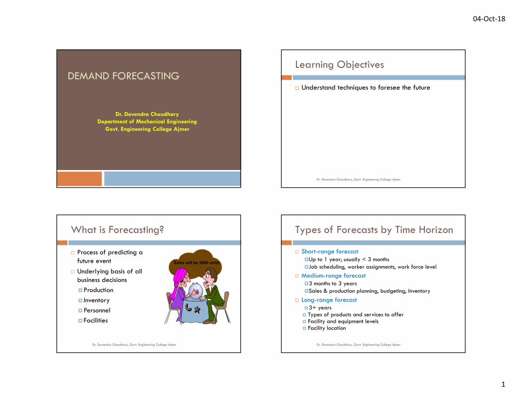
DEMAND FORECASTING
Dr. Devendra ChoudharyDepartment of Mechanical Engineering
Govt. Engineering College Ajmer
Learning Objectives
Understand techniques to foresee the future
Dr. Devendra Choudhary, Govt. Engineering College Ajmer
What is Forecasting?
Process of predicting a future event
Underlying basis of allbusiness decisions
Production
Inventory
Personnel
Facilities
Sales will be 2000 units
Dr. Devendra Choudhary, Govt. Engineering College Ajmer
Types of Forecasts by Time Horizon
Short-range forecastUp to 1 year; usually < 3 monthsJob scheduling, worker assignments, work force level
Medium-range forecast3 months to 3 yearsSales & production planning, budgeting, Inventory
Long-range forecast3+ years Types of products and services to offer Facility and equipment levels Facility location
Dr. Devendra Choudhary, Govt. Engineering College Ajmer

04-Oct-18
2
Influence of Product Life Cycle
Stages of introduction & growth require longer-range forecasts thanmaturity and decline
Forecasts useful in projecting staffing levels,
inventory levels, and
factory capacity
as product passesthrough stages
Dr. Devendra Choudhary, Govt. Engineering College Ajmer
Demand forecasts
Predict new product sales
Predict existing product sales
Dr. Devendra Choudhary, Govt. Engineering College Ajmer
Seven Steps in Forecasting
Determine the use of theforecast
Select the items to beforecast
Determine the time horizon of the forecast
Select the forecasting model(Cost and accuracy)
Gather the data Make the forecast Validate and implement
results
Step 1 Determine purpose of forecast
Step 2 Select the item for forecast
Step 3 Establish a time horizon
Step 4 Select a forecasting technique
Step 5 Gather and analyze data
Step 6 Make the forecast
“The forecast”
Step 7 Monitor the forecast
Dr. Devendra Choudhary, Govt. Engineering College Ajmer
Realities of Forecasting
Forecasts are seldom perfect because of randomness
Short-term forecasts tend to be more accuratethan longer-term forecasts Forecast accuracy decreases as time horizon increases
Both product family and aggregated productforecasts are more accurate than individual productforecasts
Forecasts more accurate for groups vs. individuals
Dr. Devendra Choudhary, Govt. Engineering College Ajmer

04-Oct-18
3
Forecasting Approaches
Used when situation isvague & little data exist
New products
New technology
Involves intuition, experience
e.g., forecasting sales on Internet
Used when situation is‘stable’ & historical data exist Existing products Current technology
Involves mathematicaltechniques
e.g., forecasting sales of color televisions
Qualitative Methods Quantitative Methods
Dr. Devendra Choudhary, Govt. Engineering College Ajmer
Overview of Qualitative Methods
Jury of executive opinion
Pool opinions of high-level executives, sometimesaugment by statistical models
Sales force composite
estimates from individual salespersons are reviewedfor reasonableness, then aggregated
Delphi method
Panel of experts, queried iteratively
Consumer Market Survey
Ask the customer
Dr. Devendra Choudhary, Govt. Engineering College Ajmer
Jury of Executive Opinion
Involves small group of high-level managers
Group estimates demand by working together
Combines managerial experience withstatistical models
Relatively quick
‘Group-think’disadvantage
Dr. Devendra Choudhary, Govt. Engineering College Ajmer
Sales Force Composite
Each salespersonprojects their sales
Combined at district & national levels
Sales rep’s knowcustomers’ wants
Tends to be overlyoptimistic
Sales
© 1995 Corel Corp.
Dr. Devendra Choudhary, Govt. Engineering College Ajmer

04-Oct-18
4
Delphi Method
Iterative group process
3 types of people
Decision makers
Staff
Respondents
Reduces ‘group-think’
Respondents
Staff
Decision Makers(Sales?)
(What
will sales be? survey)
(Sales will be 45, 50, 55)
(Sales will be 50!)
Dr. Devendra Choudhary, Govt. Engineering College Ajmer
Consumer Market Survey
Ask customers aboutpurchasing plans
What consumers say, and what they actuallydo are often different
Sometimes difficult toanswer
How many hours will
next week
How many hours willyou use the Internet
next week?
Dr. Devendra Choudhary, Govt. Engineering College Ajmer
Overview of Quantitative Approaches
Time-series models Naïve approach
Moving averages
Weighted moving average
Exponential smoothing
Trend projection
Causal models
Quantitative
Forecasting
Linear
Regression
Causal
Models
Exponential
Smoothing
Moving
Average
Time Series
Models
Trend
Projection
Dr. Devendra Choudhary, Govt. Engineering College Ajmer
Time series models
Trend
Seasonal
Cyclical
Random
Seasonality - short-term regular variations in data
Trend - long-term movement in data CYCLE- wave like variations lasting more than one year
Random variations - caused by chance or unusual circumstances
Dr. Devendra Choudhary, Govt. Engineering College Ajmer

04-Oct-18
5
Time series models
Trend
Randomvariation
Cycles
Seasonal variations
90
89
88
cycle
Dr. Devendra Choudhary, Govt. Engineering College Ajmer
Time series models
Year1
Year2
Year3
Year4
Seasonal peaks Trend component
Actual demand line
Average demand over four years
Dem
and f
or
pro
duct
or
serv
ice
Random variation
Dr. Devendra Choudhary, Govt. Engineering College Ajmer
Trend Component
Persistent, overall upward or downward pattern
Due to population, technology etc.
Several years duration
Mo., Qtr., Yr.
Response
© 1984-1994 T/Maker Co.
Dr. Devendra Choudhary, Govt. Engineering College Ajmer
Cyclical Component
Repeating up & down movements
Due to interactions of factors influencing economy
Usually 2-10 years duration
Mo., Qtr., Yr.
Response
Cycle
BDr. Devendra Choudhary, Govt. Engineering College Ajmer

04-Oct-18
6
Seasonal Component
Regular pattern of up & down fluctuations
Due to weather, customs etc.
Occurs within 1 year
Mo., Qtr.
Response
Summer
© 1984-1994 T/Maker Co.
Dr. Devendra Choudhary, Govt. Engineering College Ajmer
Random Component
Erratic, unsystematic, ‘residual’ fluctuations
Due to random variation or unforeseen events
Union strike
Tornado
Short duration & nonrepeating
Dr. Devendra Choudhary, Govt. Engineering College Ajmer
Naive Approach
Assumes demand in nextperiod is the same as demand in most recentperiod
e.g., If May sales were48, then June sales willbe 48
Cannot provide high accuracy
Sometimes cost effective& efficient © 1995 Corel Corp.
Dr. Devendra Choudhary, Govt. Engineering College Ajmer
Moving Average Method
MA is a series of arithmetic means
Used if little or no trend
Used often forsmoothing Provides overall
impression of data over time
MAn
n
Demand in Previous Periods
Increasing n makesforecast less sensitive tochanges
Do not forecast trendwell
Require much historicaldata
Dr. Devendra Choudhary, Govt. Engineering College Ajmer

04-Oct-18
7
Weighted Moving Average Method
WMASum of weights
Weight * Demand
More recent values in a series are given more weight in computing the forecast.
Dr. Devendra Choudhary, Govt. Engineering College Ajmer
Exponential Smoothing
We should give more weight to the more recent time periods when forecasting.
Need just three pieces of data to start:
Last period’s forecast (Ft)
Last periods actual demand value (At)
Select value of smoothing coefficient, ,between 0 and 1.0
If no last period forecast is available, average the last few periods or use naive method
Ft+1 = Ft + (At - Ft)
tt1t Fα1αAF ++
Dr. Devendra Choudhary, Govt. Engineering College Ajmer
Forecast Effect of Smoothing Constant
Higher values (e.g. 0.7 or 0.8) may place too much weight on last period’s random variation
Ft = At - 1 + (1- ) At - 2 + (1- )2At - 3 + ...
Weights
Prior Period
2 periods ago
(1 - )
3 periods ago
(1 - )2
=
= 0.10
= 0.90
10% 9% 8.1%
90% 9% 0.9%Dr. Devendra Choudhary, Govt. Engineering College Ajmer
Problem 1
Determine forecast for periods 7 & 8
3-period moving average
5-period moving average
3-period weighted moving average with t-1 weighted 0.5, t-2 weighted 0.3 and t-3 weighted 0.2
Exponential smoothing with alpha=0.2 and 0.6, the period 6 forecast being 375
Period Actual
1 300
2 315
3 290
4 346
5 320
6 360
7 376
8
Dr. Devendra Choudhary, Govt. Engineering College Ajmer

04-Oct-18
8
Problem 1
Period Actual 3-P MA
5-P MA
3-P WMA
ES ( = .2)
ES ( = .6)
1 300
2 315
3 290
4 346
5 320
6 360
7 376 342
8 352
Dr. Devendra Choudhary, Govt. Engineering College Ajmer
Problem 1
Period Actual 3-P MA
5-P MA
3-P WMA
ES ( = .2)
ES ( = .2)
1 300
2 315
3 290
4 346
5 320
6 360
7 376 326.28 338.4
Dr. Devendra Choudhary, Govt. Engineering College Ajmer
Problem 1
Period Actual 3-P MA
5-P MA
3-P WMA
ES ( = .2)
ES ( = .2)
1 300
2 315
3 290
4 346
5 320
6 360
7 376 345.2
8 360
0.5*360+0.3*320+0.2*346
Dr. Devendra Choudhary, Govt. Engineering College Ajmer
Problem 1
Period Actual 3-P MA
5-P MA
3-P WMA
ES ( = .2)
ES ( = .2)
1 300
2 315
3 290
4 346
5 320
6 360 375
7 376 372
8 372.8
Given
F7 = F6 + *(A6 – F6)
F8 = F7 + *(A7 – F7)
Dr. Devendra Choudhary, Govt. Engineering College Ajmer

04-Oct-18
9
Problem 1
Period Actual 3-P MA
5-P MA
3-P WMA
ES ( = .2)
ES ( = .2)
1 300
2 315
3 290
4 346
5 320
6 360 375
7 376 366
8 372
Given
F7 = F6 + *(A6 – F6)
F8 = F7 + *(A7 – F7)
Dr. Devendra Choudhary, Govt. Engineering College Ajmer
Problem 1
Period Actual 3-P MA
5-P MA
3-P WMA
ES ( = .2)
ES ( = .2)
1 300
2 315
3 290
4 346
5 320
6 360
7 376 342 326.2 345.2 372 366
8 352 338.4 360 372.8 372
Dr. Devendra Choudhary, Govt. Engineering College Ajmer
Forecast Accuracy
Error - difference between actual value and predicted value
Mean Absolute Deviation (MAD)
Average absolute error
Mean Squared Error (MSE)
Average of squared error
Mean Absolute Percent Error (MAPE)
Average absolute percent error
ttt FAE
n
forecastactualMAD
n
forecast - actualMSE
2
MAPE =|At - Ft|
AtDr. Devendra Choudhary, Govt. Engineering College Ajmer
Which is better
Period ActualForecast a=.10
Forecast a=.50
1 180 175 1752 1683 1594 1755 1906 2057 1808 1829 ? ? ?
Given
To determine
Dr. Devendra Choudhary, Govt. Engineering College Ajmer

04-Oct-18
10
Which is better
Period ActualForecast a=.10
Forecast a=.50
1 180 175.00 175.002 168 175.50 177.503 159 174.75 172.754 175 173.18 165.885 190 173.36 170.446 205 175.02 180.227 180 178.02 192.618 182 178.22 186.309 ? 178.60 184.15
Dr. Devendra Choudhary, Govt. Engineering College Ajmer
Which is better
Period ActualForecast a=.10
ErrorAbsolute
ErrorSquared
errorAbsolute % error
1 180 175.00 5.00 5.00 25.00 2.78
2 168 175.50 -7.50 7.50 56.25 4.46
3 159 174.75 -15.75 15.75 248.06 9.91
4 175 173.18 1.82 1.82 3.33 1.04
5 190 173.36 16.64 16.64 276.97 8.76
6 205 175.02 29.98 29.98 898.70 14.62
7 180 178.02 1.98 1.98 3.92 1.10
8 182 178.22 3.78 3.78 14.31 2.08
4.49 10.31 190.82 5.59
ME MAD MSE MAPE
Dr. Devendra Choudhary, Govt. Engineering College Ajmer
Which is better
Period ActualForecast a=.50
ErrorAbsolute
ErrorSquared
errorAbsolute % error
1 180 175.00 5.00 5.00 25.00 2.78
2 168 177.50 -9.50 9.50 90.25 5.65
3 159 172.75 -13.75 13.75 189.06 8.65
4 175 165.88 9.13 9.13 83.27 5.21
5 190 170.44 19.56 19.56 382.69 10.30
6 205 180.22 24.78 24.78 614.11 12.09
7 180 192.61 -12.61 12.61 159.00 7.01
8 182 186.30 -4.30 4.30 18.53 2.37
2.29 12.33 195.24 6.76
ME MAD MSE MAPE
Dr. Devendra Choudhary, Govt. Engineering College Ajmer
Which is better
Forecast a=.10 Forecast a=.50
ME 4.49 2.29
MAD 10.31 12.33
MSE 190.82 195.24
MAPE 5.59 6.76
On the basis of MAD, MSE and MAPE, a smoothing constant of = 0.10 is Preferred to = 0.50
Dr. Devendra Choudhary, Govt. Engineering College Ajmer

04-Oct-18
11
Trend-adjusted exponential smoothing
Month Actual Forecast = 0.4
Forecast = 0.9
1 100 100 (Given) 100 (Given)
2 200 100 100
3 300 140 190
4 400 204 289
5 500 282.4 388.9
ES fails to respond to trends.
To improve our forecast, ES is adjusted for trend.
With T-ES, both the forecast and trend are smoothed using two smoothing constants and β, respectively.
Dr. Devendra Choudhary, Govt. Engineering College Ajmer
Trend-adjusted exponential smoothing
It uses a three step process
Step 1 - Smoothing the forecast
Step 2 – Smoothing the trend
Step 3 – Forecast including the trend
Ft = (Actual demand last period)
+ (1- )(Forecast last period+Trend estimate last period)
Ft = (At-1) + (1- )(Ft-1 + Tt-1)
Tt = (Forecast this period - Forecast last period)
+ (1-)(Trend estimate last period)
Tt = (Ft - Ft-1) + (1- )Tt-1
Forecast including trend (FITt) = exponentially smoothed forecast (Ft)
+ exponentially smoothed trend (Tt)Dr. Devendra Choudhary, Govt. Engineering College Ajmer
Forecasting trend problem
A company uses exponential smoothing with trend to forecast usage of itslawn care products. At the end of July the company wishes to forecast salesfor August. July demand was 62. The trend in July has been 15 additionalgallons of product sold per month. Forecast has been 57 gallons per month.The company uses alpha+0.2 and beta +0.10. Forecast for August.
Smooth the forecast:
FAugust = *AJuly + (1- )(FJuly + TJuly) = 0.2*62 + 0.8*(57+15) = 70
Smooth the trend:
TAugust = β(FAugust – FJuly) + (1 – β)*TJuly = 0.1*(70 – 57) + 0.9*15 = 14.8
Forecast including trend:
FITAugust = FAugust + TAugust = 70+14.8 = 84.8 gallons
Dr. Devendra Choudhary, Govt. Engineering College Ajmer
T-ES Problem
A manufacturer wantsto forecast demandfor an item. Past salesindicates an increasingtrend. The firmassumes the initialforecast of month 1was 11 units and thetrend over that periodwas 2 units. Take =.2 and β = .4.
Month Actual
1 12
2 17
3 20
4 19
5 24
6 21
7 31
8 28
9 36
10 ?Dr. Devendra Choudhary, Govt. Engineering College Ajmer

04-Oct-18
12
T-ES Problem
Month Actual Forecast Trend FIT
1 12 11.00 2.00 13.00
2 17 F2=.2*12+(1-.2)*(11+2)
12.80 T2=.4*(12.8-11)+(1-.4)*2
1.92 14.72
3 20 15.18 2.10 17.28
4 19 17.82 2.32 20.14
5 24 19.91 2.23 22.14
6 21 22.51 2.38 24.89
7 31 24.11 2.07 26.18
8 28 27.14 2.45 29.59
9 36 29.28 2.32 31.60
10 ? 32.48 2.68 35.16
Ft = (At-1) + (1- )(Ft-1 + Tt-1) Tt = (Ft - Ft-1) + (1- )Tt-1
Dr. Devendra Choudhary, Govt. Engineering College Ajmer
Comparing ES and T-ES
0.00
5.00
10.00
15.00
20.00
25.00
30.00
35.00
40.00
1 2 3 4 5 6 7 8 9
FIT ES Actual
Dr. Devendra Choudhary, Govt. Engineering College Ajmer
Forecasting Seasonality
Calculate the average demand per season E.g.: average monthly/quarterly demand
Calculate the average demand over the all season Calculate a seasonal index for each season :
Divide the average monthly/quarterly demand of each season by the average demand over the all season
Forecast demand for the next year & divide by the number of seasons Use regular forecasting method & divide by four for average quarterly
demand
Multiply next year’s average seasonal demand by each seasonal index Result is a forecast of demand for each month/quarter of next year
Dr. Devendra Choudhary, Govt. Engineering College Ajmer
Forecasting Seasonality
Seasonality problem: a university must develop forecasts for the next year’s quarterly enrollments. It has collected quarterly enrollments for the past two years. It has also forecast total enrollment for next year to be 90,000 students. What is the forecast for each quarter of next year?
Quarter Year 1 Year 2 Average Seasonal Index
Year3
Fall 24000 26000 25000 1.22 27439
Winter 23000 22000 22500 1.10 24695
Spring 19000 19000 19000 0.93 20854
Summer 14000 17000 15500 0.76 17012
Total 80000 84000 20500 90000
Dr. Devendra Choudhary, Govt. Engineering College Ajmer

04-Oct-18
13
Controlling the Forecast
Control chart
A visual tool for monitoring forecast errors
Used to detect non-randomness in errors
Forecasting errors are in control if
All errors are within the control limits
No patterns, such as trends or cycles, are present
Dr. Devendra Choudhary, Govt. Engineering College Ajmer
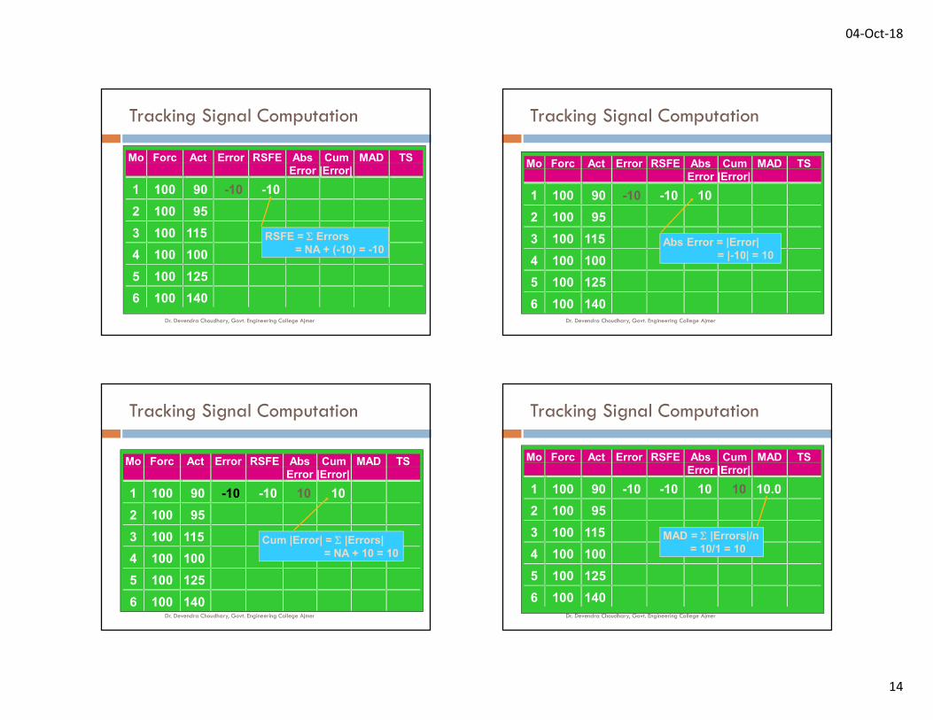
Tracking Signal
Ratio of cumulative error to MAD
Measures how well forecast is predicting actual values
Monitors the forecast to see if it is biased high or low
Should be within upper and lower control limits
If the forecasting model is performing well, the TS should be around zero
Tracking signal =(Actual - forecast)
MAD
Dr. Devendra Choudhary, Govt. Engineering College Ajmer
Mo Fcst Act Error RSFE AbsError
Cum MAD TS
1 100 90
2 100 95
3 100 115
4 100 100
5 100 125
6 100 140
|Error|
Tracking Signal Computation
Dr. Devendra Choudhary, Govt. Engineering College Ajmer
Mo Forc Act Error RSFE AbsError
Cum MAD TS
1 100 90
2 100 95
3 100 115
4 100 100
5 100 125
6 100 140
-10
Error = Actual - Forecast= 90 - 100 = -10
|Error|
Tracking Signal Computation
Dr. Devendra Choudhary, Govt. Engineering College Ajmer
04-Oct-18
14
Mo Forc Act Error RSFE AbsError
Cum MAD TS
1 100 90
2 100 95
3 100 115
4 100 100
5 100 125
6 100 140
-10 -10
RSFE = Errors= NA + (-10) = -10
|Error|
Tracking Signal Computation
Dr. Devendra Choudhary, Govt. Engineering College Ajmer
Mo Forc Act Error RSFE AbsError
Cum MAD TS
1 100 90
2 100 95
3 100 115
4 100 100
5 100 125
6 100 140
-10 -10 10
Abs Error = |Error|= |-10| = 10
|Error|
Tracking Signal Computation
Dr. Devendra Choudhary, Govt. Engineering College Ajmer
Mo Forc Act Error RSFE AbsError
Cum MAD TS
1 100 90
2 100 95
3 100 115
4 100 100
5 100 125
6 100 140
-10 -10 10 10
Cum |Error| = |Errors|= NA + 10 = 10
|Error|
Tracking Signal Computation
Dr. Devendra Choudhary, Govt. Engineering College Ajmer
Mo Forc Act Error RSFE AbsError
Cum|Error|
MAD TS
1 100 90
2 100 95
3 100 115
4 100 100
5 100 125
6 100 140
-10 -10 10 10 10.0
MAD = |Errors|/n= 10/1 = 10
Tracking Signal Computation
Dr. Devendra Choudhary, Govt. Engineering College Ajmer

04-Oct-18
15
Mo Forc Act Error RSFE AbsError
Cum MAD TS
1 100 90
2 100 95
3 100 115
4 100 100
5 100 125
6 100 140
-10 -10 10 10 10.0 -1
TS = RSFE/MAD= -10/10 = -1
|Error|
Tracking Signal Computation
Dr. Devendra Choudhary, Govt. Engineering College Ajmer
Mo Forc Act Error RSFE AbsError
Cum MAD TS
1 100 90
2 100 95
3 100 115
4 100 100
5 100 125
6 100 140
-10 -10 10 10 10.0 -1
-5
Error = Actual - Forecast= 95 - 100 = -5
|Error|
Tracking Signal Computation
Dr. Devendra Choudhary, Govt. Engineering College Ajmer
Mo Forc Act Error RSFE AbsError
Cum MAD TS
1 100 90
2 100 95
3 100 115
4 100 100
5 100 125
6 100 140
-10 -10 10 10 10.0 -1
-5 -15
RSFE = Errors= (-10) + (-5) = -15
|Error|
Tracking Signal Computation
Dr. Devendra Choudhary, Govt. Engineering College Ajmer
Mo Forc Act Error RSFE AbsError
Cum MAD TS
1 100 90
2 100 95
3 100 115
4 100 100
5 100 125
6 100 140
-10 -10 10 10 10.0 -1
-5 -15 5
Abs Error = |Error|= |-5| = 5
|Error|
Tracking Signal Computation
Dr. Devendra Choudhary, Govt. Engineering College Ajmer

04-Oct-18
16
Mo Forc Act Error RSFE AbsError
Cum MAD TS
1 100 90
2 100 95
3 100 115
4 100 100
5 100 125
6 100 140
-10 -10 10 10 10.0 -1
-5 -15 5 15
Cum Error = |Errors|= 10 + 5 = 15
|Error|
Tracking Signal Computation
Dr. Devendra Choudhary, Govt. Engineering College Ajmer
Mo Forc Act Error RSFE AbsError
Cum MAD TS
1 100 90
2 100 95
3 100 115
4 100 100
5 100 125
6 100 140
-10 -10 10 10 10.0 -1
-5 -15 5 15 7.5
MAD = |Errors|/n= 15/2 = 7.5
|Error|
Tracking Signal Computation
Dr. Devendra Choudhary, Govt. Engineering College Ajmer
Mo Forc Act Error RSFE AbsError
Cum MAD TS
1 100 90
2 100 95
3 100 115
4 100 100
5 100 125
6 100 140
-10 -10 10 10 10.0 -1
-5 -15 5 15 7.5 -2
|Error|
TS = RSFE/MAD= -15/7.5 = -2
Tracking Signal Computation
Dr. Devendra Choudhary, Govt. Engineering College Ajmer
Plot of a Tracking Signal
Time
Lower control limit
Upper control limit
Signal exceeded limit
Tracking signal
Acceptable range
+
0
-
Dr. Devendra Choudhary, Govt. Engineering College Ajmer

04-Oct-18
17
Causal Models
Causal models establish a cause-and-effect relationship between independent and dependent variables
A common tool of causal modeling is linear regression:
bxaY +
Dr. Devendra Choudhary, Govt. Engineering College Ajmer
Linear Regression
Identify dependent (y) and independent (x) variables
Solve for the slope of the line
Solve for the y intercept
Develop your equation for the trend line
Y=a + bX
XbYa
22 XnX
YXnXYb
Dr. Devendra Choudhary, Govt. Engineering College Ajmer
Linear Regression Problem
A maker of golf shirts has been tracking the relationship between sales and advertising expenditure. Use linear regression to find out what sales might be if the company invested Rs. 53 lacs in advertising next year.
Adv. (X) Sales (Y)
1 32 130
2 52 151
3 50 150
4 55 158
5 53 ?Dr. Devendra Choudhary, Govt. Engineering College Ajmer
Linear Regression Problem
Adv. (X) Sales (Y) XY X2
1 32 130 4160 1024
2 52 151 7852 2704
3 50 150 7500 2500
4 55 158 8690 3025
Sum 189 589 28202 9253
Average 47.25 147.25 7050.5 2313.25
b = 1.15182 a = 92.82649
5 53 153.75
XbYa
22 XnX
YXnXYb
Y=a + bXY=92.8 + 1.15*53
Dr. Devendra Choudhary, Govt. Engineering College Ajmer

04-Oct-18
18
Correlation
Answers: ‘how strong’ is the linear relationship between thevariables?’
Coefficient of correlation is denoted by r Values range from -1 to +1 Measures degree of association
Used mainly for understanding
-1.0 +1.00
Perfect Positive Correlation
Increasing degree of negativecorrelation
-.5 +.5
Perfect NegativeCorrelation No Correlation
Increasing degree of positive correlation
Dr. Devendra Choudhary, Govt. Engineering College Ajmer
Correlation
r = 1 r = -1
r = .89 r = 0
Y
X
Yi = a + b Xi^
Y
X
Y
X
Y
X
Yi = a + b Xi^ Yi = a + b Xi
^
Yi = a + b Xi^
Dr. Devendra Choudhary, Govt. Engineering College Ajmer
Regression and Linear Trend Projection
Used for forecasting linear trend line
Assumes relationship between response variable, Yiand time, Xi is a linear function
Estimated by least squares method
Minimizes sum of squared errors
Proceed same way as we solved for causal model
$iY a bXi +
Dr. Devendra Choudhary, Govt. Engineering College Ajmer
Regression and Seasonal Index
Year Q1 Q2 Q3 Q4
1 520 730 820 530
2 590 810 900 600
3 650 900 1000 650
0
200
400
600
800
1000
1200
0 1 2 3 4 5 6 7 8 9 10 11 12 13
Period
Sa
les
Dr. Devendra Choudhary, Govt. Engineering College Ajmer

04-Oct-18
19
Regression and Seasonal Index
Year Q1 Q2 Q3 Q4
1 520 730 820 530
2 590 810 900 600
3 650 900 1000 650
Sum 1760 2440 2720 1780
Dr. Devendra Choudhary, Govt. Engineering College Ajmer
Regression and Seasonal Index
Year Q1 Q2 Q3 Q4 Annual total
1 520 730 820 530 2600
2 590 810 900 600 2900
3 650 900 1000 650 3200
Sum 1760 2440 2720 1780 8700
Avg 586.7 813.3 906.7 593.3 725.0
Dr. Devendra Choudhary, Govt. Engineering College Ajmer
Regression and Seasonal Index
Year Q1 Q2 Q3 Q4 Annual total
1 520 730 820 530 2600
2 590 810 900 600 2900
3 650 900 1000 650 3200
Sum 1760 2440 2720 1780 8700
Avg 586.7 813.3 906.7 593.3 725.0
SI 0.809 1.122 1.251 0.818
Dr. Devendra Choudhary, Govt. Engineering College Ajmer
Regression and Seasonal Index
De-seasonalized data
Year Q1 Q2 Q3 Q4
1 642.6 650.7 655.7 647.6
2 729.1 722.0 719.7 733.1
3 803.3 802.3 799.6 794.2
For year 1 and Q1, 520 / 0.809 = 642.6
Dr. Devendra Choudhary, Govt. Engineering College Ajmer

04-Oct-18
20
Regression and Seasonal Index
De-seasonalized data
500.0
550.0
600.0
650.0
700.0
750.0
800.0
850.0
0 1 2 3 4 5 6 7 8 9 10 11 12 13
Period
Sa
les
Dr. Devendra Choudhary, Govt. Engineering College Ajmer
Regression and Seasonal Index
Y = 615.41 + 16.86 x
r = 0.94
x y x^2 y^2 xy
1 642.6 1 412952.3 642.6
2 650.7 4 423432.9 1301.4
3 655.7 9 429940.6 1967.1
4 647.6 16 419401.8 2590.4
5 729.1 25 531615.0 3645.6
6 722.0 36 521325.4 4332.2
7 719.7 49 517923.6 5037.7
8 733.1 64 537503.2 5865.2
9 803.3 81 645237.9 7229.4
10 802.3 100 643611.6 8022.5
11 799.6 121 639411.9 8796.0
12 794.2 144 630819.7 9530.9
78 8700 650 6353176 58961.01Sum
Dr. Devendra Choudhary, Govt. Engineering College Ajmer
Regression and Seasonal Index
De-seasonalized data
500.0
550.0
600.0
650.0
700.0
750.0
800.0
850.0
0 1 2 3 4 5 6 7 8 9 10 11 12 13
Period
Sa
les
Dr. Devendra Choudhary, Govt. Engineering College Ajmer
Regression and Seasonal Index
Y = 615.41 + 16.86 x
Quarter Prediction
13 834.6
14 851.5
15 868.3
16 885.2
Deseasonalized Forecast
Dr. Devendra Choudhary, Govt. Engineering College Ajmer

04-Oct-18
21
Regression and Seasonal Index
Quarter Prediction SISeasonal
Forecast
13 834.6 0.809 675.3
14 851.5 1.122 955.2
15 868.3 1.251 1085.9
16 885.2 0.818 724.4
Dr. Devendra Choudhary, Govt. Engineering College Ajmer
Regression and Seasonal Index
Year Q1 Q2 Q3 Q4
1 520 730 820 530
2 590 810 900 600
3 650 900 1000 650
4 675 955 1086 724
Next Year’s Forecast
0
200
400
600
800
1000
1200
0 1 2 3 4 5 6 7 8 9 10 11 12 13 1415 16 17
Period
Sa
les
Dr. Devendra Choudhary, Govt. Engineering College Ajmer
Choosing a Forecasting Technique
No single technique works in every situation
Two most important factors
Cost
Accuracy
Other factors include the availability of:
Historical data
Computers
Time needed to gather and analyze the data
Forecast horizon
Dr. Devendra Choudhary, Govt. Engineering College Ajmer