Learning with Noisy Labels

Nagarajan Natarajan Inderjit S. Dhillon Pradeep RavikumarDepartment of Computer Science, University of Texas, Austin.{naga86,inderjit,pradeepr}@cs.utexas.edu

Ambuj TewariDepartment of Statistics, University of Michigan, Ann Arbor.

tewaria@umich.edu

AbstractIn this paper, we theoretically study the problem of binary classification in thepresence of random classification noise — the learner, instead of seeing the true la-bels, sees labels that have independently been flipped with some small probability.Moreover, random label noise isclass-conditional— the flip probability dependson the class. We provide two approaches to suitably modify any given surrogateloss function. First, we provide a simple unbiased estimator of any loss, and ob-tain performance bounds for empirical risk minimization inthe presence of iiddata with noisy labels. If the loss function satisfies a simple symmetry condition,we show that the method leads to an efficient algorithm for empirical minimiza-tion. Second, by leveraging a reduction of risk minimization under noisy labelsto classification with weighted 0-1 loss, we suggest the use of a simple weightedsurrogate loss, for which we are able to obtain strong empirical risk bounds. Thisapproach has a very remarkable consequence — methods used inpractice suchas biased SVM and weighted logistic regression are provablynoise-tolerant. Ona synthetic non-separable dataset, our methods achieve over 88% accuracy evenwhen 40% of the labels are corrupted, and are competitive with respect to recentlyproposed methods for dealing with label noise in several benchmark datasets.

1 IntroductionDesigning supervised learning algorithms that can learn from data sets with noisy labels is a problemof great practical importance. Here, by noisy labels, we refer to the setting where an adversary hasdeliberately corrupted the labels [Biggio et al., 2011], which otherwise arise from some “clean”distribution; learning from only positive and unlabeled data [Elkan and Noto, 2008] can also be castin this setting. Given the importance of learning from such noisy labels, a great deal of practicalwork has been done on the problem (see, for instance, the survey article by Nettleton et al. [2010]).The theoretical machine learning community has also investigated the problem of learning fromnoisy labels. Soon after the introduction of the noise-freePAC model, Angluin and Laird [1988]proposed therandom classification noise(RCN) model where each label is flipped independentlywith some probabilityρ ∈ [0, 1/2). It is known [Aslam and Decatur, 1996, Cesa-Bianchi et al.,1999] that finiteness of the VC dimension characterizes learnability in the RCN model. Similarly, inthe online mistake bound model, the parameter that characterizes learnability without noise — theLittestone dimension — continues to characterize learnability even in the presence of random labelnoise [Ben-David et al., 2009]. These results are for the so-called “0-1” loss. Learning with convexlosses has been addressed only under limiting assumptions like separability or uniform noise rates[Manwani and Sastry, 2013].

In this paper, we consider risk minimization in the presenceof class-conditionalrandom label noise(abbreviated CCN). The data consists of iid samples from an underlying “clean” distributionD.The learning algorithm sees samples drawn from a noisy versionDρ of D — where the noise ratesdepend on the class label. To the best of our knowledge, general results in this setting have not beenobtained before. To this end, we develop two methods for suitably modifyingany given surrogateloss functionℓ, and show that minimizing the sample average of the modified proxy loss function

1

ℓ leads to provable risk bounds where the risk is calculated using the original lossℓ on the cleandistribution.

In our first approach, the modified or proxy loss is an unbiasedestimate of the loss function. Theidea of using unbiased estimators is well-known in stochastic optimization [Nemirovski et al., 2009],and regret bounds can be obtained for learning with noisy labels in an online learning setting (SeeAppendix B). Nonetheless, we bring out some important aspects of using unbiased estimators ofloss functions for empirical risk minimization under CCN. In particular, we give a simple symmetrycondition on the loss (enjoyed, for instance, by the Huber, logistic, and squared losses) to ensure thatthe proxy loss is also convex. Hinge loss does not satisfy thesymmetry condition, and thus leadsto a non-convex problem. We nonetheless provide a convex surrogate, leveraging the fact that thenon-convex hinge problem is “close” to a convex problem (Theorem 6).

Our second approach is based on the fundamental observationthat the minimizer of the risk (i.e.probability of misclassification) under the noisy distribution differs from that of the clean distribu-tion only in where it thresholdsη(x) = P (Y = 1|x) to decide the label. In order to correct for thethreshold, we then propose a simple weighted loss function,where the weights are label-dependent,as the proxy loss function. Our analysis builds on the notionof consistency of weighted loss func-tions studied by Scott [2012]. This approach leads to a very remarkable result that appropriatelyweighted losses like biased SVMs studied by Liu et al. [2003]are robust to CCN.

The main results and the contributions of the paper are summarized below:

1. To the best of our knowledge, we are the first to provide guarantees for risk minimization underrandom label noise in the general setting of convex surrogates, without any assumptions on thetrue distribution.

2. We provide two different approaches to suitably modifying any given surrogate loss function,that surprisingly lead to very similar risk bounds (Theorems 3 and 11). These general resultsinclude some existing results for random classification noise as special cases.

3. We resolve an elusive theoretical gap in the understanding of practical methods like biased SVMand weighted logistic regression — they are provably noise-tolerant (Theorem 11).

4. Our proxy losses are easy to compute — both the methods yield efficient algorithms.5. Experiments on benchmark datasets show that the methods are robust even at high noise rates.

The outline of the paper is as follows. We introduce the problem setting and terminology in Section2. In Section 3, we give our first main result concerning the method of unbiased estimators. InSection 4, we give our second and third main results for certain weighted loss functions. We presentexperimental results on synthetic and benchmark data sets in Section 5.

1.1 Related WorkStarting from the work of Bylander [1994], many noise tolerant versions of the perceptron algorithmhave been developed. This includes the passive-aggressivefamily of algorithms [Crammer et al.,2006], confidence weighted learning [Dredze et al., 2008], AROW [Crammer et al., 2009] and theNHERD algorithm [Crammer and Lee, 2010]. The survey articleby Khardon and Wachman [2007]provides an overview of some of this literature. A Bayesian approach to the problem of noisy labelsis taken by Graepel and Herbrich [2000] and Lawrence and Sch¨olkopf [2001]. As Adaboost is verysensitive to label noise, random label noise has also been considered in the context of boosting. Longand Servedio [2010] prove that any method based on a convex potential is inherently ill-suited torandom label noise. Freund [2009] proposes a boosting algorithm based on a non-convex potentialthat is empirically seen to be robust against random label noise.

Stempfel and Ralaivola [2009] proposed the minimization ofan unbiased proxy for the case ofthe hinge loss. However the hinge loss leads to a non-convex problem. Therefore, they proposedheuristic minimization approaches for which no theoretical guarantees were provided (We addressthe issue in Section 3.1). Cesa-Bianchi et al. [2011] focus on the online learning algorithms wherethey only need unbiased estimates of the gradient of the lossto provide guarantees for learning withnoisy data. However, they consider a much harder noise modelwhereinstances as well as labelsare noisy. Because of the harder noise model, they necessarily require multiple noisy copies perclean example and the unbiased estimation schemes also become fairly complicated. In particular,their techniques break down for non-smooth losses such as the hinge loss. In contrast, we showthat unbiased estimation is always possible in the more benign random classification noise setting.Manwani and Sastry [2013] consider whether empirical risk minimization of the loss itself on the

2

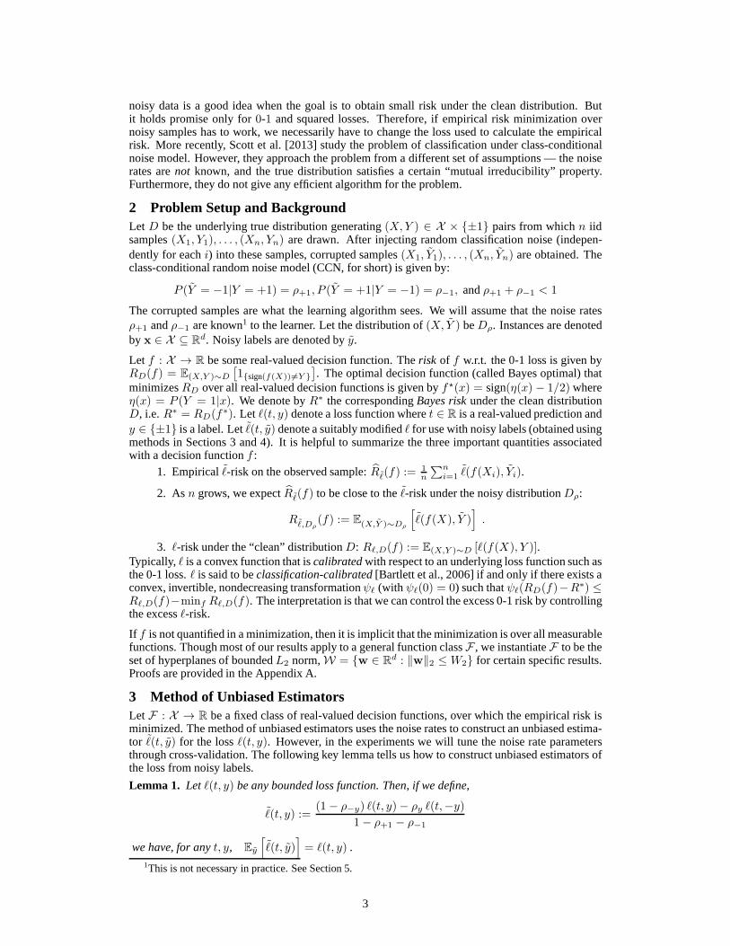
noisy data is a good idea when the goal is to obtain small risk under the clean distribution. Butit holds promise only for0-1 and squared losses. Therefore, if empirical risk minimization overnoisy samples has to work, we necessarily have to change the loss used to calculate the empiricalrisk. More recently, Scott et al. [2013] study the problem ofclassification under class-conditionalnoise model. However, they approach the problem from a different set of assumptions — the noiserates arenot known, and the true distribution satisfies a certain “mutualirreducibility” property.Furthermore, they do not give any efficient algorithm for theproblem.

2 Problem Setup and BackgroundLet D be the underlying true distribution generating(X,Y ) ∈ X × {±1} pairs from whichn iidsamples(X1, Y1), . . . , (Xn, Yn) are drawn. After injecting random classification noise (indepen-dently for eachi) into these samples, corrupted samples(X1, Y1), . . . , (Xn, Yn) are obtained. Theclass-conditional random noise model (CCN, for short) is given by:

P (Y = −1|Y = +1) = ρ+1, P (Y = +1|Y = −1) = ρ−1, andρ+1 + ρ−1 < 1

The corrupted samples are what the learning algorithm sees.We will assume that the noise ratesρ+1 andρ−1 are known1 to the learner. Let the distribution of(X, Y ) beDρ. Instances are denotedby x ∈ X ⊆ R

d. Noisy labels are denoted byy.

Let f : X → R be some real-valued decision function. Therisk of f w.r.t. the 0-1 loss is given byRD(f) = E(X,Y )∼D

[1{sign(f(X)) 6=Y }

]. The optimal decision function (called Bayes optimal) that

minimizesRD over all real-valued decision functions is given byf⋆(x) = sign(η(x) − 1/2) whereη(x) = P (Y = 1|x). We denote byR∗ the correspondingBayes riskunder the clean distributionD, i.e.R∗ = RD(f∗). Let ℓ(t, y) denote a loss function wheret ∈ R is a real-valued prediction andy ∈ {±1} is a label. Letℓ(t, y) denote a suitably modifiedℓ for use with noisy labels (obtained usingmethods in Sections 3 and 4). It is helpful to summarize the three important quantities associatedwith a decision functionf :

1. Empiricalℓ-risk on the observed sample:Rℓ(f) :=1n

∑ni=1 ℓ(f(Xi), Yi).

2. Asn grows, we expectRℓ(f) to be close to theℓ-risk under the noisy distributionDρ:

Rℓ,Dρ(f) := E(X,Y )∼Dρ

[ℓ(f(X), Y )

].

3. ℓ-risk under the “clean” distributionD: Rℓ,D(f) := E(X,Y )∼D [ℓ(f(X), Y )].Typically,ℓ is a convex function that iscalibratedwith respect to an underlying loss function such asthe 0-1 loss.ℓ is said to beclassification-calibrated[Bartlett et al., 2006] if and only if there exists aconvex, invertible, nondecreasing transformationψℓ (with ψℓ(0) = 0) such thatψℓ(RD(f)−R∗) ≤Rℓ,D(f)−minf Rℓ,D(f). The interpretation is that we can control the excess 0-1 risk by controllingthe excessℓ-risk.

If f is not quantified in a minimization, then it is implicit that the minimization is over all measurablefunctions. Though most of our results apply to a general function classF , we instantiateF to be theset of hyperplanes of boundedL2 norm,W = {w ∈ R

d : ‖w‖2 ≤W2} for certain specific results.Proofs are provided in the Appendix A.

3 Method of Unbiased EstimatorsLet F : X → R be a fixed class of real-valued decision functions, over which the empirical risk isminimized. The method of unbiased estimators uses the noiserates to construct an unbiased estima-tor ℓ(t, y) for the lossℓ(t, y). However, in the experiments we will tune the noise rate parametersthrough cross-validation. The following key lemma tells ushow to construct unbiased estimators ofthe loss from noisy labels.

Lemma 1. Let ℓ(t, y) be any bounded loss function. Then, if we define,

ℓ(t, y) :=(1− ρ−y) ℓ(t, y)− ρy ℓ(t,−y)

1− ρ+1 − ρ−1

we have, for anyt, y, Ey

[ℓ(t, y)

]= ℓ(t, y) .

1This is not necessary in practice. See Section 5.

3

We can try to learn a good predictor in the presence of label noise by minimizing the sample average

f ← argminf∈F

Rℓ(f) .

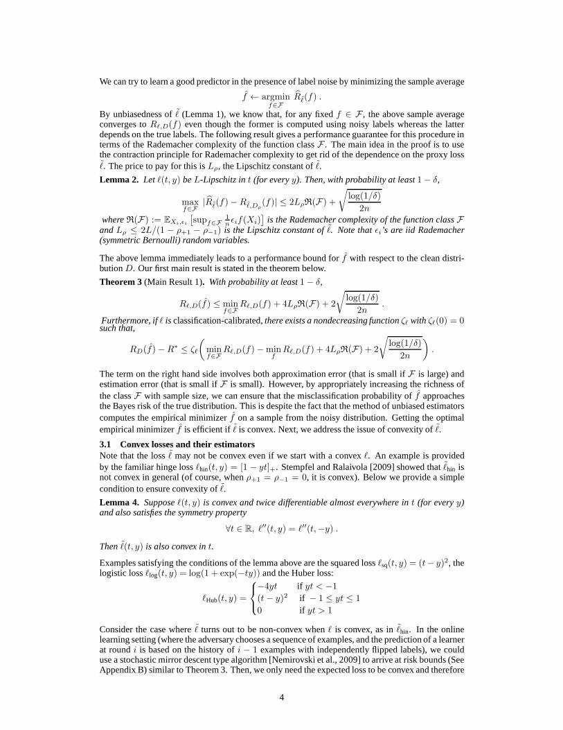
By unbiasedness ofℓ (Lemma 1), we know that, for any fixedf ∈ F , the above sample averageconverges toRℓ,D(f) even though the former is computed using noisy labels whereas the latterdepends on the true labels. The following result gives a performance guarantee for this procedure interms of the Rademacher complexity of the function classF . The main idea in the proof is to usethe contraction principle for Rademacher complexity to getrid of the dependence on the proxy lossℓ. The price to pay for this isLρ, the Lipschitz constant ofℓ.

Lemma 2. Let ℓ(t, y) beL-Lipschitz int (for everyy). Then, with probability at least1− δ,

maxf∈F

|Rℓ(f)−Rℓ,Dρ(f)| ≤ 2LρR(F) +

√log(1/δ)

2nwhereR(F) := EXi,ǫi

[supf∈F

1nǫif(Xi)

]is the Rademacher complexity of the function classF

andLρ ≤ 2L/(1 − ρ+1 − ρ−1) is the Lipschitz constant ofℓ. Note thatǫi’s are iid Rademacher(symmetric Bernoulli) random variables.

The above lemma immediately leads to a performance bound forf with respect to the clean distri-butionD. Our first main result is stated in the theorem below.

Theorem 3 (Main Result 1). With probability at least1− δ,

Rℓ,D(f) ≤ minf∈F

Rℓ,D(f) + 4LρR(F) + 2

√log(1/δ)

2n.

Furthermore, ifℓ is classification-calibrated, there exists a nondecreasing functionζℓ with ζℓ(0) = 0such that,

RD(f)−R∗ ≤ ζℓ(minf∈F

Rℓ,D(f)−minfRℓ,D(f) + 4LρR(F) + 2

√log(1/δ)

2n

).

The term on the right hand side involves both approximation error (that is small ifF is large) andestimation error (that is small ifF is small). However, by appropriately increasing the richness ofthe classF with sample size, we can ensure that the misclassification probability of f approachesthe Bayes risk of the true distribution. This is despite the fact that the method of unbiased estimatorscomputes the empirical minimizerf on a sample from the noisy distribution. Getting the optimalempirical minimizerf is efficient if ℓ is convex. Next, we address the issue of convexity ofℓ.

3.1 Convex losses and their estimatorsNote that the lossℓ may not be convex even if we start with a convexℓ. An example is providedby the familiar hinge lossℓhin(t, y) = [1 − yt]+. Stempfel and Ralaivola [2009] showed thatℓhin isnot convex in general (of course, whenρ+1 = ρ−1 = 0, it is convex). Below we provide a simplecondition to ensure convexity ofℓ.

Lemma 4. Supposeℓ(t, y) is convex and twice differentiable almost everywhere int (for everyy)and also satisfies the symmetry property

∀t ∈ R, ℓ′′(t, y) = ℓ′′(t,−y) .

Thenℓ(t, y) is also convex int.

Examples satisfying the conditions of the lemma above are the squared lossℓsq(t, y) = (t− y)2, thelogistic lossℓlog(t, y) = log(1 + exp(−ty)) and the Huber loss:

ℓHub(t, y) =

−4yt if yt < −1(t− y)2 if − 1 ≤ yt ≤ 1

0 if yt > 1

Consider the case whereℓ turns out to be non-convex whenℓ is convex, as inℓhin. In the onlinelearning setting (where the adversary chooses a sequence ofexamples, and the prediction of a learnerat roundi is based on the history ofi − 1 examples with independently flipped labels), we coulduse a stochastic mirror descent type algorithm [Nemirovskiet al., 2009] to arrive at risk bounds (SeeAppendix B) similar to Theorem 3. Then, we only need the expected loss to be convex and therefore

4

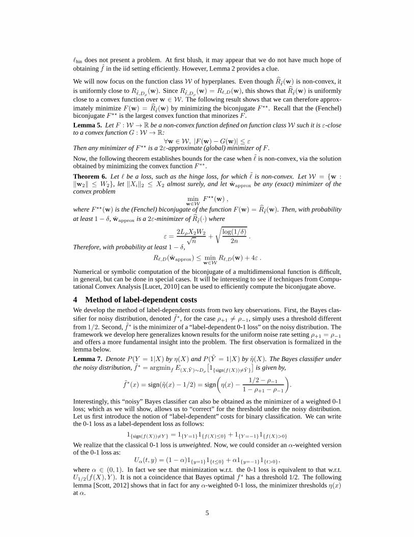
ℓhin does not present a problem. At first blush, it may appear that we do not have much hope ofobtainingf in the iid setting efficiently. However, Lemma 2 provides a clue.

We will now focus on the function classW of hyperplanes. Even thoughRℓ(w) is non-convex, itis uniformly close toRℓ,Dρ

(w). SinceRℓ,Dρ(w) = Rℓ,D(w), this shows thatRℓ(w) is uniformly

close to a convex function overw ∈ W . The following result shows that we can therefore approx-imately minimizeF (w) = Rℓ(w) by minimizing the biconjugateF ⋆⋆. Recall that the (Fenchel)biconjugateF ⋆⋆ is the largest convex function that minorizesF .

Lemma 5. LetF :W → R be a non-convex function defined on function classW such it isε-closeto a convex functionG :W → R:

∀w ∈ W , |F (w)−G(w)| ≤ εThen any minimizer ofF ⋆⋆ is a2ε-approximate (global) minimizer ofF .

Now, the following theorem establishes bounds for the case whenℓ is non-convex, via the solutionobtained by minimizing the convex functionF ∗∗.

Theorem 6. Let ℓ be a loss, such as the hinge loss, for whichℓ is non-convex. LetW = {w :‖w2‖ ≤ W2}, let ‖Xi‖2 ≤ X2 almost surely, and letwapprox be any (exact) minimizer of theconvex problem

minw∈W

F ⋆⋆(w) ,

whereF ⋆⋆(w) is the (Fenchel) biconjugate of the functionF (w) = Rℓ(w). Then, with probability

at least1− δ, wapprox is a2ε-minimizer ofRℓ(·) where

ε =2LρX2W2√

n+

√log(1/δ)

2n.

Therefore, with probability at least1− δ,Rℓ,D(wapprox) ≤ min

w∈WRℓ,D(w) + 4ε .

Numerical or symbolic computation of the biconjugate of a multidimensional function is difficult,in general, but can be done in special cases. It will be interesting to see if techniques from Compu-tational Convex Analysis [Lucet, 2010] can be used to efficiently compute the biconjugate above.

4 Method of label-dependent costsWe develop the method of label-dependent costs from two key observations. First, the Bayes clas-sifier for noisy distribution, denotedf∗, for the caseρ+1 6= ρ−1, simply uses a threshold differentfrom1/2. Second,f∗ is the minimizer of a “label-dependent 0-1 loss” on the noisydistribution. Theframework we develop here generalizes known results for theuniform noise rate settingρ+1 = ρ−1

and offers a more fundamental insight into the problem. The first observation is formalized in thelemma below.

Lemma 7. DenoteP (Y = 1|X) by η(X) andP (Y = 1|X) by η(X). The Bayes classifier underthe noisy distribution,f∗ = argminf E(X,Y )∼Dρ

[1{sign(f(X)) 6=Y }

]is given by,

f∗(x) = sign(η(x)− 1/2) = sign

(η(x) − 1/2− ρ−1

1− ρ+1 − ρ−1

).

Interestingly, this “noisy” Bayes classifier can also be obtained as the minimizer of a weighted 0-1loss; which as we will show, allows us to “correct” for the threshold under the noisy distribution.Let us first introduce the notion of “label-dependent” costsfor binary classification. We can writethe 0-1 loss as a label-dependent loss as follows:

1{sign(f(X)) 6=Y } = 1{Y=1}1{f(X)≤0} + 1{Y=−1}1{f(X)>0}

We realize that the classical 0-1 loss isunweighted. Now, we could consider anα-weighted versionof the 0-1 loss as:

Uα(t, y) = (1− α)1{y=1}1{t≤0} + α1{y=−1}1{t>0},

whereα ∈ (0, 1). In fact we see that minimization w.r.t. the 0-1 loss is equivalent to that w.r.t.U1/2(f(X), Y ). It is not a coincidence that Bayes optimalf∗ has a threshold 1/2. The followinglemma [Scott, 2012] shows that in fact for anyα-weighted 0-1 loss, the minimizer thresholdsη(x)atα.

5

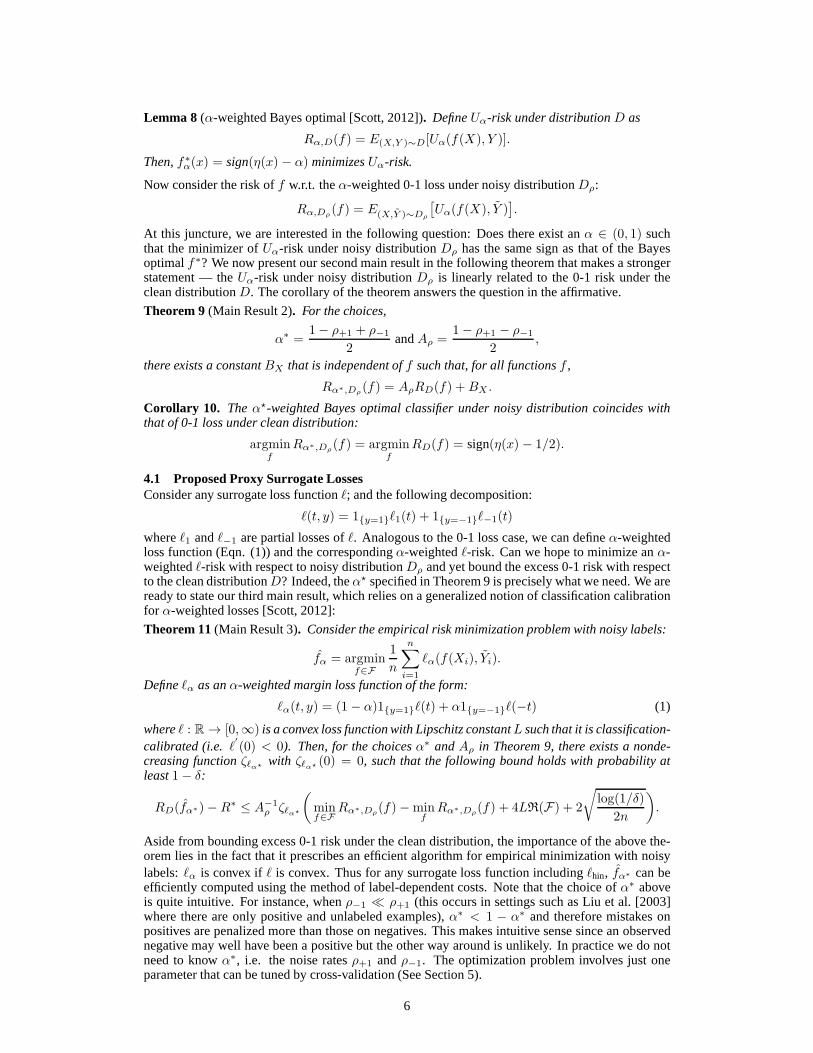
Lemma 8 (α-weighted Bayes optimal [Scott, 2012]). DefineUα-risk under distributionD as

Rα,D(f) = E(X,Y )∼D[Uα(f(X), Y )].

Then,f∗α(x) = sign(η(x) − α) minimizesUα-risk.

Now consider the risk off w.r.t. theα-weighted 0-1 loss under noisy distributionDρ:

Rα,Dρ(f) = E(X,Y )∼Dρ

[Uα(f(X), Y )

].

At this juncture, we are interested in the following question: Does there exist anα ∈ (0, 1) suchthat the minimizer ofUα-risk under noisy distributionDρ has the same sign as that of the Bayesoptimalf∗? We now present our second main result in the following theorem that makes a strongerstatement — theUα-risk under noisy distributionDρ is linearly related to the 0-1 risk under theclean distributionD. The corollary of the theorem answers the question in the affirmative.

Theorem 9 (Main Result 2). For the choices,

α∗ =1− ρ+1 + ρ−1

2andAρ =

1− ρ+1 − ρ−1

2,

there exists a constantBX that is independent off such that, for all functionsf ,

Rα∗,Dρ(f) = AρRD(f) +BX .

Corollary 10. Theα⋆-weighted Bayes optimal classifier under noisy distribution coincides withthat of 0-1 loss under clean distribution:

argminf

Rα∗,Dρ(f) = argmin

fRD(f) = sign(η(x) − 1/2).

4.1 Proposed Proxy Surrogate LossesConsider any surrogate loss functionℓ; and the following decomposition:

ℓ(t, y) = 1{y=1}ℓ1(t) + 1{y=−1}ℓ−1(t)

whereℓ1 andℓ−1 are partial losses ofℓ. Analogous to the 0-1 loss case, we can defineα-weightedloss function (Eqn. (1)) and the correspondingα-weightedℓ-risk. Can we hope to minimize anα-weightedℓ-risk with respect to noisy distributionDρ and yet bound the excess 0-1 risk with respectto the clean distributionD? Indeed, theα⋆ specified in Theorem 9 is precisely what we need. We areready to state our third main result, which relies on a generalized notion of classification calibrationfor α-weighted losses [Scott, 2012]:

Theorem 11 (Main Result 3). Consider the empirical risk minimization problem with noisy labels:

fα = argminf∈F

1

n

n∑

i=1

ℓα(f(Xi), Yi).

Defineℓα as anα-weighted margin loss function of the form:

ℓα(t, y) = (1− α)1{y=1}ℓ(t) + α1{y=−1}ℓ(−t) (1)

whereℓ : R→ [0,∞) is a convex loss function with Lipschitz constantL such that it is classification-calibrated (i.e. ℓ

′

(0) < 0). Then, for the choicesα∗ andAρ in Theorem 9, there exists a nonde-creasing functionζℓα⋆ with ζℓα⋆ (0) = 0, such that the following bound holds with probability atleast1− δ:

RD(fα∗)−R∗ ≤ A−1ρ ζℓα⋆

(minf∈F

Rα∗,Dρ(f)−min

fRα∗,Dρ

(f) + 4LR(F) + 2

√log(1/δ)

2n

).

Aside from bounding excess 0-1 risk under the clean distribution, the importance of the above the-orem lies in the fact that it prescribes an efficient algorithm for empirical minimization with noisylabels:ℓα is convex ifℓ is convex. Thus for any surrogate loss function includingℓhin, fα∗ can beefficiently computed using the method of label-dependent costs. Note that the choice ofα∗ aboveis quite intuitive. For instance, whenρ−1 ≪ ρ+1 (this occurs in settings such as Liu et al. [2003]where there are only positive and unlabeled examples),α∗ < 1 − α∗ and therefore mistakes onpositives are penalized more than those on negatives. This makes intuitive sense since an observednegative may well have been a positive but the other way around is unlikely. In practice we do notneed to knowα∗, i.e. the noise ratesρ+1 andρ−1. The optimization problem involves just oneparameter that can be tuned by cross-validation (See Section 5).

6

5 ExperimentsWe show the robustness of the proposed algorithms to increasing rates of label noise on synthetic andreal-world datasets. We compare the performance of the two proposed methods with state-of-the-artmethods for dealing with random classification noise. We divide each dataset (randomly) into 3training and test sets. We use a cross-validation set to tunethe parameters specific to the algorithms.Accuracy of a classification algorithm is defined as the fraction of examples in the test set classifiedcorrectlywith respect to the clean distribution. For given noise ratesρ+1 andρ−1, labels of thetraining data are flipped accordingly and average accuracy over 3 train-test splits is computed2. Forevaluation, we choose a representative algorithm based on each of the two proposed methods —ℓlogfor the method of unbiased estimators and the widely-used C-SVM [Liu et al., 2003] method (whichapplies different costs on positives and negatives) for themethod of label-dependent costs.

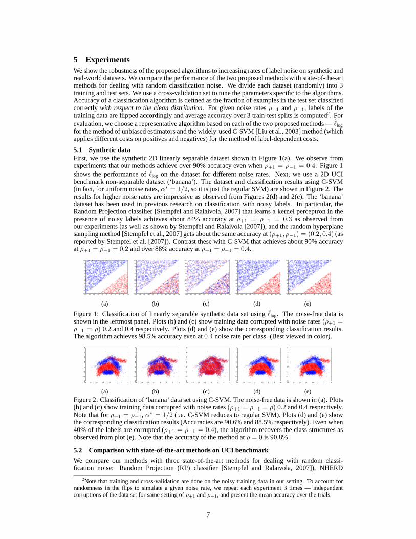
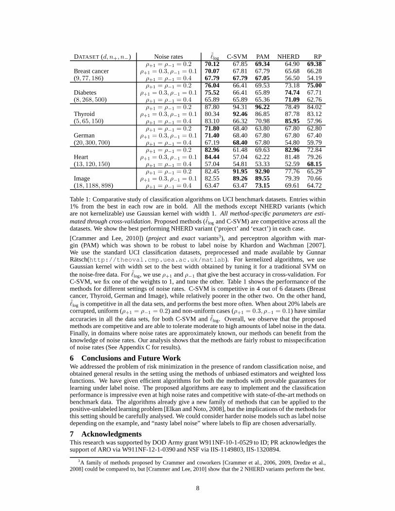
5.1 Synthetic dataFirst, we use the synthetic 2D linearly separable dataset shown in Figure 1(a). We observe fromexperiments that our methods achieve over 90% accuracy evenwhenρ+1 = ρ−1 = 0.4. Figure 1shows the performance ofℓlog on the dataset for different noise rates. Next, we use a 2D UCIbenchmark non-separable dataset (‘banana’). The dataset and classification results using C-SVM(in fact, for uniform noise rates,α∗ = 1/2, so it is just the regular SVM) are shown in Figure 2. Theresults for higher noise rates are impressive as observed from Figures 2(d) and 2(e). The ‘banana’dataset has been used in previous research on classificationwith noisy labels. In particular, theRandom Projection classifier [Stempfel and Ralaivola, 2007] that learns a kernel perceptron in thepresence of noisy labels achieves about 84% accuracy atρ+1 = ρ−1 = 0.3 as observed fromour experiments (as well as shown by Stempfel and Ralaivola [2007]), and the random hyperplanesampling method [Stempfel et al., 2007] gets about the same accuracy at(ρ+1, ρ−1) = (0.2, 0.4) (asreported by Stempfel et al. [2007]). Contrast these with C-SVM that achieves about 90% accuracyatρ+1 = ρ−1 = 0.2 and over 88% accuracy atρ+1 = ρ−1 = 0.4.

−100 −80 −60 −40 −20 0 20 40 60 80 100−100

−80

−60

−40

−20

0

20

40

60

80

100

(a)

−100 −80 −60 −40 −20 0 20 40 60 80 100−100

−80

−60

−40

−20

0

20

40

60

80

100

(b)

−100 −80 −60 −40 −20 0 20 40 60 80 100−100

−80

−60

−40

−20

0

20

40

60

80

100

(c)

−100 −80 −60 −40 −20 0 20 40 60 80 100−100

−80

−60

−40

−20

0

20

40

60

80

100

(d)

−100 −80 −60 −40 −20 0 20 40 60 80 100−100

−80

−60

−40

−20

0

20

40

60

80

100

(e)

Figure 1: Classification of linearly separable synthetic data set usingℓlog. The noise-free data isshown in the leftmost panel. Plots (b) and (c) show training data corrupted with noise rates(ρ+1 =ρ−1 = ρ) 0.2 and 0.4 respectively. Plots (d) and (e) show the corresponding classification results.The algorithm achieves 98.5% accuracy even at0.4 noise rate per class. (Best viewed in color).

−4 −3 −2 −1 0 1 2 3−3

−2

−1

0

1

2

3

4

(a)

−4 −3 −2 −1 0 1 2 3−3

−2

−1

0

1

2

3

4

(b)

−4 −3 −2 −1 0 1 2 3−3

−2

−1

0

1

2

3

4

(c)

−4 −3 −2 −1 0 1 2 3−3

−2

−1

0

1

2

3

4

(d)

−4 −3 −2 −1 0 1 2 3−3

−2

−1

0

1

2

3

4

(e)

Figure 2: Classification of ‘banana’ data set using C-SVM. The noise-free data is shown in (a). Plots(b) and (c) show training data corrupted with noise rates(ρ+1 = ρ−1 = ρ) 0.2 and 0.4 respectively.Note that forρ+1 = ρ−1, α∗ = 1/2 (i.e. C-SVM reduces to regular SVM). Plots (d) and (e) showthe corresponding classification results (Accuracies are 90.6% and 88.5% respectively). Even when40% of the labels are corrupted (ρ+1 = ρ−1 = 0.4), the algorithm recovers the class structures asobserved from plot (e). Note that the accuracy of the method at ρ = 0 is 90.8%.

5.2 Comparison with state-of-the-art methods on UCI benchmark

We compare our methods with three state-of-the-art methodsfor dealing with random classi-fication noise: Random Projection (RP) classifier [Stempfeland Ralaivola, 2007]), NHERD

2Note that training and cross-validation are done on the noisy training data in our setting. To account forrandomness in the flips to simulate a given noise rate, we repeat each experiment 3 times — independentcorruptions of the data set for same setting ofρ+1 andρ

−1, and present the mean accuracy over the trials.

7

DATASET (d, n+, n−) Noise rates ℓlog C-SVM PAM NHERD RPρ+1 = ρ−1 = 0.2 70.12 67.85 69.34 64.90 69.38

Breast cancer ρ+1 = 0.3, ρ−1 = 0.1 70.07 67.81 67.79 65.68 66.28(9, 77, 186) ρ+1 = ρ−1 = 0.4 67.79 67.79 67.05 56.50 54.19

ρ+1 = ρ−1 = 0.2 76.04 66.41 69.53 73.18 75.00Diabetes ρ+1 = 0.3, ρ−1 = 0.1 75.52 66.41 65.89 74.74 67.71(8, 268, 500) ρ+1 = ρ−1 = 0.4 65.89 65.89 65.36 71.09 62.76

ρ+1 = ρ−1 = 0.2 87.80 94.31 96.22 78.49 84.02Thyroid ρ+1 = 0.3, ρ−1 = 0.1 80.34 92.46 86.85 87.78 83.12(5, 65, 150) ρ+1 = ρ−1 = 0.4 83.10 66.32 70.98 85.95 57.96

ρ+1 = ρ−1 = 0.2 71.80 68.40 63.80 67.80 62.80German ρ+1 = 0.3, ρ−1 = 0.1 71.40 68.40 67.80 67.80 67.40(20, 300, 700) ρ+1 = ρ−1 = 0.4 67.19 68.40 67.80 54.80 59.79

ρ+1 = ρ−1 = 0.2 82.96 61.48 69.63 82.96 72.84Heart ρ+1 = 0.3, ρ−1 = 0.1 84.44 57.04 62.22 81.48 79.26(13, 120, 150) ρ+1 = ρ−1 = 0.4 57.04 54.81 53.33 52.59 68.15

ρ+1 = ρ−1 = 0.2 82.45 91.95 92.90 77.76 65.29Image ρ+1 = 0.3, ρ−1 = 0.1 82.55 89.26 89.55 79.39 70.66(18, 1188, 898) ρ+1 = ρ−1 = 0.4 63.47 63.47 73.15 69.61 64.72

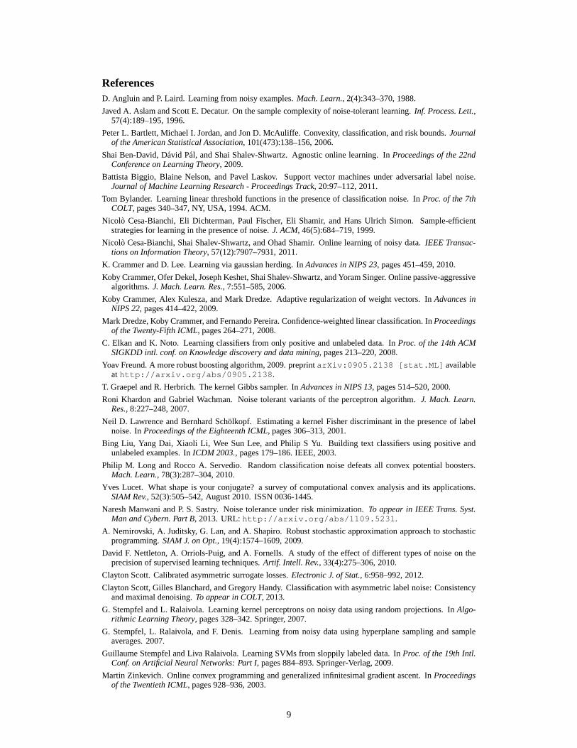
Table 1: Comparative study of classification algorithms on UCI benchmark datasets. Entries within1% from the best in each row are in bold. All the methods exceptNHERD variants (whichare not kernelizable) use Gaussian kernel with width 1.All method-specific parameters are esti-mated through cross-validation. Proposed methods (ℓlog and C-SVM) are competitive across all thedatasets. We show the best performing NHERD variant (‘project’ and ‘exact’) in each case.

[Crammer and Lee, 2010]) (project and exact variants3), and perceptron algorithm with mar-gin (PAM) which was shown to be robust to label noise by Khardon and Wachman [2007].We use the standard UCI classification datasets, preprocessed and made available by GunnarRatsch(http://theoval.cmp.uea.ac.uk/matlab). For kernelized algorithms, we useGaussian kernel with width set to the best width obtained by tuning it for a traditional SVM onthe noise-free data. Forℓlog, we useρ+1 andρ−1 that give the best accuracy in cross-validation. ForC-SVM, we fix one of the weights to 1, and tune the other. Table 1shows the performance of themethods for different settings of noise rates. C-SVM is competitive in 4 out of 6 datasets (Breastcancer, Thyroid, German and Image), while relatively poorer in the other two. On the other hand,ℓlog is competitive in all the data sets, and performs the best more often. When about 20% labels arecorrupted, uniform (ρ+1 = ρ−1 = 0.2) and non-uniform cases (ρ+1 = 0.3, ρ−1 = 0.1) have similaraccuracies in all the data sets, for both C-SVM andℓlog. Overall, we observe that the proposedmethods are competitive and are able to tolerate moderate tohigh amounts of label noise in the data.Finally, in domains where noise rates are approximately known, our methods can benefit from theknowledge of noise rates. Our analysis shows that the methods are fairly robust to misspecificationof noise rates (See Appendix C for results).

6 Conclusions and Future WorkWe addressed the problem of risk minimization in the presence of random classification noise, andobtained general results in the setting using the methods ofunbiased estimators and weighted lossfunctions. We have given efficient algorithms for both the methods with provable guarantees forlearning under label noise. The proposed algorithms are easy to implement and the classificationperformance is impressive even at high noise rates and competitive with state-of-the-art methods onbenchmark data. The algorithms already give a new family of methods that can be applied to thepositive-unlabeled learning problem [Elkan and Noto, 2008], but the implications of the methods forthis setting should be carefully analysed. We could consider harder noise models such as label noisedepending on the example, and “nasty label noise” where labels to flip are chosen adversarially.

7 AcknowledgmentsThis research was supported by DOD Army grant W911NF-10-1-0529 to ID; PR acknowledges thesupport of ARO via W911NF-12-1-0390 and NSF via IIS-1149803, IIS-1320894.

3A family of methods proposed by Crammer and coworkers [Crammer et al., 2006, 2009, Dredze et al.,2008] could be compared to, but [Crammer and Lee, 2010] show that the 2 NHERD variants perform the best.

8

ReferencesD. Angluin and P. Laird. Learning from noisy examples.Mach. Learn., 2(4):343–370, 1988.

Javed A. Aslam and Scott E. Decatur. On the sample complexityof noise-tolerant learning.Inf. Process. Lett.,57(4):189–195, 1996.

Peter L. Bartlett, Michael I. Jordan, and Jon D. McAuliffe. Convexity, classification, and risk bounds.Journalof the American Statistical Association, 101(473):138–156, 2006.

Shai Ben-David, David Pal, and Shai Shalev-Shwartz. Agnostic online learning. InProceedings of the 22ndConference on Learning Theory, 2009.

Battista Biggio, Blaine Nelson, and Pavel Laskov. Support vector machines under adversarial label noise.Journal of Machine Learning Research - Proceedings Track, 20:97–112, 2011.

Tom Bylander. Learning linear threshold functions in the presence of classification noise. InProc. of the 7thCOLT, pages 340–347, NY, USA, 1994. ACM.

Nicolo Cesa-Bianchi, Eli Dichterman, Paul Fischer, Eli Shamir, and Hans Ulrich Simon. Sample-efficientstrategies for learning in the presence of noise.J. ACM, 46(5):684–719, 1999.

Nicolo Cesa-Bianchi, Shai Shalev-Shwartz, and Ohad Shamir. Online learning of noisy data.IEEE Transac-tions on Information Theory, 57(12):7907–7931, 2011.

K. Crammer and D. Lee. Learning via gaussian herding. InAdvances in NIPS 23, pages 451–459, 2010.

Koby Crammer, Ofer Dekel, Joseph Keshet, Shai Shalev-Shwartz, and Yoram Singer. Online passive-aggressivealgorithms.J. Mach. Learn. Res., 7:551–585, 2006.

Koby Crammer, Alex Kulesza, and Mark Dredze. Adaptive regularization of weight vectors. InAdvances inNIPS 22, pages 414–422, 2009.

Mark Dredze, Koby Crammer, and Fernando Pereira. Confidence-weighted linear classification. InProceedingsof the Twenty-Fifth ICML, pages 264–271, 2008.

C. Elkan and K. Noto. Learning classifiers from only positiveand unlabeled data. InProc. of the 14th ACMSIGKDD intl. conf. on Knowledge discovery and data mining, pages 213–220, 2008.

Yoav Freund. A more robust boosting algorithm, 2009. preprintarXiv:0905.2138 [stat.ML] availableathttp://arxiv.org/abs/0905.2138.

T. Graepel and R. Herbrich. The kernel Gibbs sampler. InAdvances in NIPS 13, pages 514–520, 2000.

Roni Khardon and Gabriel Wachman. Noise tolerant variants of the perceptron algorithm.J. Mach. Learn.Res., 8:227–248, 2007.

Neil D. Lawrence and Bernhard Scholkopf. Estimating a kernel Fisher discriminant in the presence of labelnoise. InProceedings of the Eighteenth ICML, pages 306–313, 2001.

Bing Liu, Yang Dai, Xiaoli Li, Wee Sun Lee, and Philip S Yu. Building text classifiers using positive andunlabeled examples. InICDM 2003., pages 179–186. IEEE, 2003.

Philip M. Long and Rocco A. Servedio. Random classification noise defeats all convex potential boosters.Mach. Learn., 78(3):287–304, 2010.

Yves Lucet. What shape is your conjugate? a survey of computational convex analysis and its applications.SIAM Rev., 52(3):505–542, August 2010. ISSN 0036-1445.

Naresh Manwani and P. S. Sastry. Noise tolerance under risk minimization. To appear in IEEE Trans. Syst.Man and Cybern. Part B, 2013. URL:http://arxiv.org/abs/1109.5231.

A. Nemirovski, A. Juditsky, G. Lan, and A. Shapiro. Robust stochastic approximation approach to stochasticprogramming.SIAM J. on Opt., 19(4):1574–1609, 2009.

David F. Nettleton, A. Orriols-Puig, and A. Fornells. A study of the effect of different types of noise on theprecision of supervised learning techniques.Artif. Intell. Rev., 33(4):275–306, 2010.

Clayton Scott. Calibrated asymmetric surrogate losses.Electronic J. of Stat., 6:958–992, 2012.

Clayton Scott, Gilles Blanchard, and Gregory Handy. Classification with asymmetric label noise: Consistencyand maximal denoising.To appear in COLT, 2013.

G. Stempfel and L. Ralaivola. Learning kernel perceptrons on noisy data using random projections. InAlgo-rithmic Learning Theory, pages 328–342. Springer, 2007.

G. Stempfel, L. Ralaivola, and F. Denis. Learning from noisydata using hyperplane sampling and sampleaverages. 2007.

Guillaume Stempfel and Liva Ralaivola. Learning SVMs from sloppily labeled data. InProc. of the 19th Intl.Conf. on Artificial Neural Networks: Part I, pages 884–893. Springer-Verlag, 2009.

Martin Zinkevich. Online convex programming and generalized infinitesimal gradient ascent. InProceedingsof the Twentieth ICML, pages 928–936, 2003.

9