Learning with a Wasserstein Loss

Charlie Frogner⇤ Chiyuan Zhang⇤Center for Brains, Minds and MachinesMassachusetts Institute of Technology

frogner@mit.edu, chiyuan@mit.edu

Hossein MobahiCSAIL

Massachusetts Institute of Technologyhmobahi@csail.mit.edu

Mauricio Araya-PoloShell International E & P, Inc.

Mauricio.Araya@shell.com

Tomaso PoggioCenter for Brains, Minds and MachinesMassachusetts Institute of Technology

tp@ai.mit.edu

Abstract

Learning to predict multi-label outputs is challenging, but in many problems thereis a natural metric on the outputs that can be used to improve predictions. In thispaper we develop a loss function for multi-label learning, based on the Wassersteindistance. The Wasserstein distance provides a natural notion of dissimilarity forprobability measures. Although optimizing with respect to the exact Wassersteindistance is costly, recent work has described a regularized approximation that isefficiently computed. We describe an efficient learning algorithm based on thisregularization, as well as a novel extension of the Wasserstein distance from prob-ability measures to unnormalized measures. We also describe a statistical learningbound for the loss. The Wasserstein loss can encourage smoothness of the predic-tions with respect to a chosen metric on the output space. We demonstrate thisproperty on a real-data tag prediction problem, using the Yahoo Flickr CreativeCommons dataset, outperforming a baseline that doesn’t use the metric.

1 Introduction

We consider the problem of learning to predict a non-negative measure over a finite set. This prob-lem includes many common machine learning scenarios. In multiclass classification, for example,one often predicts a vector of scores or probabilities for the classes. And in semantic segmenta-tion [1], one can model the segmentation as being the support of a measure defined over the pixellocations. Many problems in which the output of the learning machine is both non-negative andmulti-dimensional might be cast as predicting a measure.

We specifically focus on problems in which the output space has a natural metric or similarity struc-ture, which is known (or estimated) a priori. In practice, many learning problems have such struc-ture. In the ImageNet Large Scale Visual Recognition Challenge [ILSVRC] [2], for example, theoutput dimensions correspond to 1000 object categories that have inherent semantic relationships,some of which are captured in the WordNet hierarchy that accompanies the categories. Similarly, inthe keyword spotting task from the IARPA Babel speech recognition project, the outputs correspondto keywords that likewise have semantic relationships. In what follows, we will call the similaritystructure on the label space the ground metric or semantic similarity.

Using the ground metric, we can measure prediction performance in a way that is sensitive to re-lationships between the different output dimensions. For example, confusing dogs with cats might

⇤Authors contributed equally.1Code and data are available at http://cbcl.mit.edu/wasserstein.

1

3 4 5 6 7

Grid Size

0.0

0.1

0.2

0.3

Dista

nce Divergence Wasserstein

0.1 0.2 0.3 0.4 0.5 0.6 0.7 0.8 0.9

Noise

0.1

0.2

0.3

0.4

Distance Divergence Wasserstein

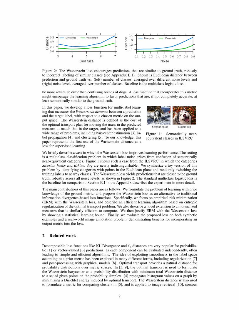
Figure 2: The Wasserstein loss encourages predictions that are similar to ground truth, robustlyto incorrect labeling of similar classes (see Appendix E.1). Shown is Euclidean distance betweenprediction and ground truth vs. (left) number of classes, averaged over different noise levels and(right) noise level, averaged over number of classes. Baseline is the multiclass logistic loss.

be more severe an error than confusing breeds of dogs. A loss function that incorporates this metricmight encourage the learning algorithm to favor predictions that are, if not completely accurate, atleast semantically similar to the ground truth.

In this paper, we develop a loss function for multi-label learn-

Siberian husky Eskimo dog

Figure 1: Semantically near-equivalent classes in ILSVRC

ing that measures the Wasserstein distance between a predictionand the target label, with respect to a chosen metric on the out-put space. The Wasserstein distance is defined as the cost ofthe optimal transport plan for moving the mass in the predictedmeasure to match that in the target, and has been applied to awide range of problems, including barycenter estimation [3], la-bel propagation [4], and clustering [5]. To our knowledge, thispaper represents the first use of the Wasserstein distance as aloss for supervised learning.

We briefly describe a case in which the Wasserstein loss improves learning performance. The settingis a multiclass classification problem in which label noise arises from confusion of semanticallynear-equivalent categories. Figure 1 shows such a case from the ILSVRC, in which the categoriesSiberian husky and Eskimo dog are nearly indistinguishable. We synthesize a toy version of thisproblem by identifying categories with points in the Euclidean plane and randomly switching thetraining labels to nearby classes. The Wasserstein loss yields predictions that are closer to the groundtruth, robustly across all noise levels, as shown in Figure 2. The standard multiclass logistic loss isthe baseline for comparison. Section E.1 in the Appendix describes the experiment in more detail.

The main contributions of this paper are as follows. We formulate the problem of learning with priorknowledge of the ground metric, and propose the Wasserstein loss as an alternative to traditionalinformation divergence-based loss functions. Specifically, we focus on empirical risk minimization(ERM) with the Wasserstein loss, and describe an efficient learning algorithm based on entropicregularization of the optimal transport problem. We also describe a novel extension to unnormalizedmeasures that is similarly efficient to compute. We then justify ERM with the Wasserstein lossby showing a statistical learning bound. Finally, we evaluate the proposed loss on both syntheticexamples and a real-world image annotation problem, demonstrating benefits for incorporating anoutput metric into the loss.

2 Related work

Decomposable loss functions like KL Divergence and `p

distances are very popular for probabilis-tic [1] or vector-valued [6] predictions, as each component can be evaluated independently, oftenleading to simple and efficient algorithms. The idea of exploiting smoothness in the label spaceaccording to a prior metric has been explored in many different forms, including regularization [7]and post-processing with graphical models [8]. Optimal transport provides a natural distance forprobability distributions over metric spaces. In [3, 9], the optimal transport is used to formulatethe Wasserstein barycenter as a probability distribution with minimum total Wasserstein distanceto a set of given points on the probability simplex. [4] propagates histogram values on a graph byminimizing a Dirichlet energy induced by optimal transport. The Wasserstein distance is also usedto formulate a metric for comparing clusters in [5], and is applied to image retrieval [10], contour

2

matching [11], and many other problems [12, 13]. However, to our knowledge, this is the first timeit is used as a loss function in a discriminative learning framework. The closest work to this pa-per is a theoretical study [14] of an estimator that minimizes the optimal transport cost between theempirical distribution and the estimated distribution in the setting of statistical parameter estimation.

3 Learning with a Wasserstein loss

3.1 Problem setup and notation

We consider the problem of learning a map from X ⇢ RD into the space Y = RK

+

of measures overa finite set K of size |K| = K. Assume K possesses a metric dK(·, ·), which is called the groundmetric. dK measures semantic similarity between dimensions of the output, which correspond tothe elements of K. We perform learning over a hypothesis space H of predictors h

✓

: X ! Y ,parameterized by ✓ 2 ⇥. These might be linear logistic regression models, for example.

In the standard statistical learning setting, we get an i.i.d. sequence of training examples S =

((x1

, y1

), . . . , (xN

, yN

)), sampled from an unknown joint distribution PX⇥Y . Given a measure ofperformance (a.k.a. risk) E(·, ·), the goal is to find the predictor h

✓

2 H that minimizes the expectedrisk E[E(h

✓

(x), y)]. Typically E(·, ·) is difficult to optimize directly and the joint distribution PX⇥Yis unknown, so learning is performed via empirical risk minimization. Specifically, we solve

min

h✓2H

(ˆES

[`(h✓

(x), y) =1

N

NX

i=1

`(h✓

(xi

), yi

)

)(1)

with a loss function `(·, ·) acting as a surrogate of E(·, ·).

3.2 Optimal transport and the exact Wasserstein loss

Information divergence-based loss functions are widely used in learning with probability-valued out-puts. Along with other popular measures like Hellinger distance and �2 distance, these divergencestreat the output dimensions independently, ignoring any metric structure on K.

Given a cost function c : K ⇥ K ! R, the optimal transport distance [15] measures the cheapestway to transport the mass in probability measure µ

1

to match that in µ2

:

Wc

(µ1

, µ2

) = inf

�2⇧(µ1,µ2)

Z

K⇥Kc(

1

,2

)�(d1

, d2

) (2)

where ⇧(µ1

, µ2

) is the set of joint probability measures on K⇥K having µ1

and µ2

as marginals. Animportant case is that in which the cost is given by a metric dK(·, ·) or its p-th power dpK(·, ·) with p �1. In this case, (2) is called a Wasserstein distance [16], also known as the earth mover’s distance[10]. In this paper, we only work with discrete measures. In the case of probability measures, theseare histograms in the simplex �

K. When the ground truth y and the output of h both lie in thesimplex �

K, we can define a Wasserstein loss.Definition 3.1 (Exact Wasserstein Loss). For any h

✓

2 H, h✓

: X ! �

K, let h✓

(|x) = h✓

(x)

bethe predicted value at element 2 K, given input x 2 X . Let y() be the ground truth value for given by the corresponding label y. Then we define the exact Wasserstein loss as

W p

p

(h(·|x), y(·)) = inf

T2⇧(h(x),y)

hT,Mi (3)

where M 2 RK⇥K

+

is the distance matrix M,

0= dpK(,

0), and the set of valid transport plans is

⇧(h(x), y) = {T 2 RK⇥K

+

: T1 = h(x), T>1 = y} (4)

where 1 is the all-one vector.

W p

p

is the cost of the optimal plan for transporting the predicted mass distribution h(x) to matchthe target distribution y. The penalty increases as more mass is transported over longer distances,according to the ground metric M .

3

Algorithm 1 Gradient of the Wasserstein loss

Given h(x), y, �, K. (�a

, �b

if h(x), y unnormalized.)u 1while u has not converged do

u

8><

>:

h(x)↵ �K �y ↵K>u��

if h(x), y normalized

h(x)�a�

�a�+1 ↵✓K�y ↵K>u

� �b��b�+1

◆ �a��a�+1

if h(x), y unnormalized

end whileIf h(x), y unnormalized: v y

�b��b�+1 ↵ �K>u

� �b��b�+1

@W p

p

/@h(x) ⇢

log u

�

� log u

>1�K

1 if h(x), y normalized�a

(1� (diag(u)Kv)↵ h(x)) if h(x), y unnormalized

4 Efficient optimization via entropic regularization

To do learning, we optimize the empirical risk minimization functional (1) by gradient descent.Doing so requires evaluating a descent direction for the loss, with respect to the predictions h(x).Unfortunately, computing a subgradient of the exact Wasserstein loss (3), is quite costly, as follows.

The exact Wasserstein loss (3) is a linear program and a subgradient of its solution can be computedusing Lagrange duality. The dual LP of (3) is

dW p

p

(h(x), y) = sup

↵,�2CM

↵>h(x) + �>y, CM

= {(↵,�) 2 RK⇥K

: ↵

+ �

0 M,

0}. (5)

As (3) is a linear program, at an optimum the values of the dual and the primal are equal (see, e.g.[17]), hence the dual optimal ↵ is a subgradient of the loss with respect to its first argument.

Computing ↵ is costly, as it entails solving a linear program with O(K2

) contraints, with K beingthe dimension of the output space. This cost can be prohibitive when optimizing by gradient descent.

4.1 Entropic regularization of optimal transport

Cuturi [18] proposes a smoothed transport objective that enables efficient approximation of both thetransport matrix in (3) and the subgradient of the loss. [18] introduces an entropic regularizationterm that results in a strictly convex problem:

�W p

p

(h(·|x), y(·)) = inf

T2⇧(h(x),y)

hT,Mi � 1

�H(T ), H(T ) = �

X

,

0

T,

0log T

,

0 . (6)

Importantly, the transport matrix that solves (6) is a diagonal scaling of a matrix K = e��M�1:

T ⇤= diag(u)Kdiag(v) (7)

for u = e�↵ and v = e�� , where ↵ and � are the Lagrange dual variables for (6).

Identifying such a matrix subject to equality constraints on the row and column sums is exactly amatrix balancing problem, which is well-studied in numerical linear algebra and for which efficientiterative algorithms exist [19]. [18] and [3] use the well-known Sinkhorn-Knopp algorithm.

4.2 Extending smoothed transport to the learning setting

When the output vectors h(x) and y lie in the simplex, (6) can be used directly in place of (3), as(6) can approximate the exact Wasserstein distance closely for large enough � [18]. In this case, thegradient ↵ of the objective can be obtained from the optimal scaling vector u as ↵ =

log u

�

� log u

>1�K

1.1 A Sinkhorn iteration for the gradient is given in Algorithm 1.

1Note that ↵ is only defined up to a constant shift: any upscaling of the vector u can be paired with acorresponding downscaling of the vector v (and vice versa) without altering the matrix T

⇤. The choice ↵ =log u� � log u>1

�K 1 ensures that ↵ is tangent to the simplex.

4

(a) Convergence to smoothed trans-port.

(b) Approximation of exactWasserstein.

(c) Convergence of alternating pro-jections (� = 50).

Figure 3: The relaxed transport problem (8) for unnormalized measures.

For many learning problems, however, a normalized output assumption is unnatural. In image seg-mentation, for example, the target shape is not naturally represented as a histogram. And even whenthe prediction and the ground truth are constrained to the simplex, the observed label can be subjectto noise that violates the constraint.

There is more than one way to generalize optimal transport to unnormalized measures, and this is asubject of active study [20]. We will develop here a novel objective that deals effectively with thedifference in total mass between h(x) and y while still being efficient to optimize.

4.3 Relaxed transport

We propose a novel relaxation that extends smoothed transport to unnormalized measures. By re-placing the equality constraints on the transport marginals in (6) with soft penalties with respect toKL divergence, we get an unconstrained approximate transport problem. The resulting objective is:

�,�a,�bWKL

(h(·|x), y(·)) = min

T2RK⇥K+

hT,Mi� 1

�H(T )+�

a

fKL (T1kh(x))+�b

fKL�T>1ky� (8)

where fKL (wkz) = w>log(w ↵ z) � 1>w + 1>z is the generalized KL divergence between

w, z 2 RK

+

. Here↵ represents element-wise division. As with the previous formulation, the optimaltransport matrix with respect to (8) is a diagonal scaling of the matrix K.Proposition 4.1. The transport matrix T ⇤ optimizing (8) satisfies T ⇤

= diag(u)Kdiag(v), whereu = (h(x)↵ T ⇤1)�a�, v =

�y ↵ (T ⇤

)

>1��b�, and K = e��M�1.

And the optimal transport matrix is a fixed point for a Sinkhorn-like iteration. 2

Proposition 4.2. T ⇤= diag(u)Kdiag(v) optimizing (8) satisfies: i) u = h(x)

�a��a�+1�(Kv)�

�a��a�+1 ,

and ii) v = y�b�

�b�+1 � �K>u�� �b�

�b�+1 , where � represents element-wise multiplication.

Unlike the previous formulation, (8) is unconstrained with respect to h(x). The gradient is given byr

h(x)

WKL

(h(·|x), y(·)) = �a

(1� T ⇤1↵ h(x)). The iteration is given in Algorithm 1.

When restricted to normalized measures, the relaxed problem (8) approximates smoothed transport(6). Figure 3a shows, for normalized h(x) and y, the relative distance between the values of (8) and(6) 3. For � large enough, (8) converges to (6) as �

a

and �b

increase.

(8) also retains two properties of smoothed transport (6). Figure 3b shows that, for normalizedoutputs, the relaxed loss converges to the unregularized Wasserstein distance as �, �

a

and �b

increase4. And Figure 3c shows that convergence of the iterations in (4.2) is nearly independent of thedimension K of the output space.

2Note that, although the iteration suggested by Proposition 4.2 is observed empirically to converge (seeFigure 3c, for example), we have not proven a guarantee that it will do so.

3In figures 3a-c, h(x), y and M are generated as described in [18] section 5. In 3a-b, h(x) and y havedimension 256. In 3c, convergence is defined as in [18]. Shaded regions are 95% intervals.

4The unregularized Wasserstein distance was computed using FastEMD [21].

5

0 1 2 3 4

p-th norm

0.080.100.120.140.160.180.20

Po

ste

rio

rP

ro

ba

bility

0

1

2

3

(a) Posterior predictions for images of digit 0.

0 1 2 3 4

p-th norm

0.080.100.120.140.160.180.20

Po

ste

rio

rP

ro

ba

bility

2

3

4

5

6

(b) Posterior predictions for images of digit 4.

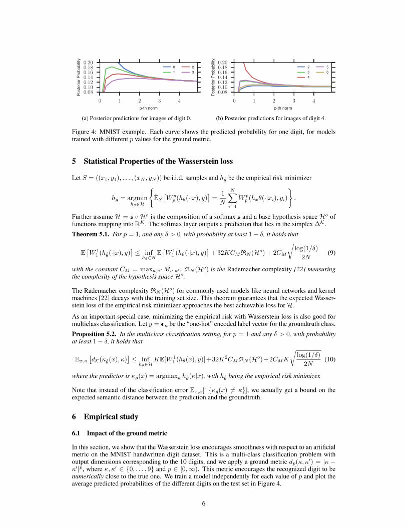
Figure 4: MNIST example. Each curve shows the predicted probability for one digit, for modelstrained with different p values for the ground metric.

5 Statistical Properties of the Wasserstein loss

Let S = ((x1

, y1

), . . . , (xN

, yN

)) be i.i.d. samples and hˆ

✓

be the empirical risk minimizer

hˆ

✓

= argmin

h✓2H

(ˆES

⇥W p

p

(h✓

(·|x), y)⇤ = 1

N

NX

i=1

W p

p

(hx

✓(·|xi

), yi

)

).

Further assume H = s � Ho is the composition of a softmax s and a base hypothesis space Ho offunctions mapping into RK . The softmax layer outputs a prediction that lies in the simplex �

K.Theorem 5.1. For p = 1, and any � > 0, with probability at least 1� �, it holds that

E⇥W 1

1

(hˆ

✓

(·|x), y)⇤ inf

h✓2HE⇥W 1

1

(h✓

(·|x), y)⇤+ 32KCM

RN

(Ho

) + 2CM

rlog(1/�)

2N(9)

with the constant CM

= max

,

0 M,

0 . RN

(Ho

) is the Rademacher complexity [22] measuringthe complexity of the hypothesis space Ho.

The Rademacher complexity RN

(Ho

) for commonly used models like neural networks and kernelmachines [22] decays with the training set size. This theorem guarantees that the expected Wasser-stein loss of the empirical risk minimizer approaches the best achievable loss for H.

As an important special case, minimizing the empirical risk with Wasserstein loss is also good formulticlass classification. Let y =

be the “one-hot” encoded label vector for the groundtruth class.Proposition 5.2. In the multiclass classification setting, for p = 1 and any � > 0, with probabilityat least 1� �, it holds that

Ex,

⇥dK(ˆ

✓

(x),)⇤ inf

h✓2HKE[W 1

1

(h✓

(x), y)]+32K2CM

RN

(Ho

)+2CM

K

rlog(1/�)

2N(10)

where the predictor is ˆ

✓

(x) = argmax

hˆ

✓

(|x), with hˆ

✓

being the empirical risk minimizer.

Note that instead of the classification error Ex,

[ {ˆ

✓

(x) 6= }], we actually get a bound on theexpected semantic distance between the prediction and the groundtruth.

6 Empirical study

6.1 Impact of the ground metric

In this section, we show that the Wasserstein loss encourages smoothness with respect to an artificialmetric on the MNIST handwritten digit dataset. This is a multi-class classification problem withoutput dimensions corresponding to the 10 digits, and we apply a ground metric d

p

(,0) = | �

0|p, where ,0 2 {0, . . . , 9} and p 2 [0,1). This metric encourages the recognized digit to benumerically close to the true one. We train a model independently for each value of p and plot theaverage predicted probabilities of the different digits on the test set in Figure 4.

6

5 10 15 20

K (# of proposed tags)

0.70

0.75

0.80

0.85

0.90

0.95

1.00

top-K

Cost

Loss Function

Divergence

Wasserstein (↵=0.5)

Wasserstein (↵=0.3)

Wasserstein (↵=0.1)

(a) Original Flickr tags dataset.

5 10 15 20

K (# of proposed tags)

0.70

0.75

0.80

0.85

0.90

0.95

1.00

top-K

Cost

Loss Function

Divergence

Wasserstein (↵=0.5)

Wasserstein (↵=0.3)

Wasserstein (↵=0.1)

(b) Reduced-redundancy Flickr tags dataset.

Figure 5: Top-K cost comparison of the proposed loss (Wasserstein) and the baseline (Divergence).

Note that as p ! 0, the metric approaches the 0 � 1 metric d0

(,0) =

6=

0 , which treats allincorrect digits as being equally unfavorable. In this case, as can be seen in the figure, the predictedprobability of the true digit goes to 1 while the probability for all other digits goes to 0. As pincreases, the predictions become more evenly distributed over the neighboring digits, convergingto a uniform distribution as p!1 5.

6.2 Flickr tag prediction

We apply the Wasserstein loss to a real world multi-label learning problem, using the recently re-leased Yahoo/Flickr Creative Commons 100M dataset [23]. 6 Our goal is tag prediction: we select1000 descriptive tags along with two random sets of 10,000 images each, associated with these tags,for training and testing. We derive a distance metric between tags by using word2vec [24] toembed the tags as unit vectors, then taking their Euclidean distances. To extract image features weuse MatConvNet [25]. Note that the set of tags is highly redundant and often many semanticallyequivalent or similar tags can apply to an image. The images are also partially tagged, as differentusers may prefer different tags. We therefore measure the prediction performance by the top-K cost,defined as C

K

= 1/KP

K

k=1

min

j

dK(k

,j

), where {j

} is the set of groundtruth tags, and {k

}are the tags with highest predicted probability. The standard AUC measure is also reported.

We find that a linear combination of the Wasserstein loss W p

p

and the standard multiclass logistic lossKL yields the best prediction results. Specifically, we train a linear model by minimizing W p

p

+↵KLon the training set, where ↵ controls the relative weight of KL. Note that KL taken alone is ourbaseline in these experiments. Figure 5a shows the top-K cost on the test set for the combined lossand the baseline KL loss. We additionally create a second dataset by removing redundant labelsfrom the original dataset: this simulates the potentially more difficult case in which a single usertags each image, by selecting one tag to apply from amongst each cluster of applicable, semanticallysimilar tags. Figure 3b shows that performance for both algorithms decreases on the harder dataset,while the combined Wasserstein loss continues to outperform the baseline.

In Figure 6, we show the effect on performance of varying the weight ↵ on the KL loss. We observethat the optimum of the top-K cost is achieved when the Wasserstein loss is weighted more heavilythan at the optimum of the AUC. This is consistent with a semantic smoothing effect of Wasserstein,which during training will favor mispredictions that are semantically similar to the ground truth,sometimes at the cost of lower AUC 7. We finally show two selected images from the test set inFigure 7. These illustrate cases in which both algorithms make predictions that are semanticallyrelevant, despite overlapping very little with the ground truth. The image on the left shows errorsmade by both algorithms. More examples can be found in the appendix.

5To avoid numerical issues, we scale down the ground metric such that all of the distance values are in theinterval [0, 1).

6The dataset used here is available at http://cbcl.mit.edu/wasserstein.7The Wasserstein loss can achieve a similar trade-off by choosing the metric parameter p, as discussed in

Section 6.1. However, the relationship between p and the smoothing behavior is complex and it can be simplerto implement the trade-off by combining with the KL loss.

7

0.0 0.5 1.0 1.5 2.0

0.650.700.750.800.850.900.95

To

p-K

co

st

K = 1 K = 2 K = 3 K = 4

0.0 0.5 1.0 1.5 2.0↵

0.54

0.56

0.58

0.60

0.62

0.64

AU

C

Wasserstein AUC

Divergence AUC

(a) Original Flickr tags dataset.

0.0 0.5 1.0 1.5 2.0

0.650.700.750.800.850.900.95

To

p-K

co

st

K = 1 K = 2 K = 3 K = 4

0.0 0.5 1.0 1.5 2.0↵

0.54

0.56

0.58

0.60

0.62

0.64

AU

C

Wasserstein AUC

Divergence AUC

(b) Reduced-redundancy Flickr tags dataset.

Figure 6: Trade-off between semantic smoothness and maximum likelihood.

(a) Flickr user tags: street, parade, dragon; ourproposals: people, protest, parade; baseline pro-posals: music, car, band.

(b) Flickr user tags: water, boat, reflection, sun-shine; our proposals: water, river, lake, summer;baseline proposals: river, water, club, nature.

Figure 7: Examples of images in the Flickr dataset. We show the groundtruth tags and as well astags proposed by our algorithm and the baseline.

7 Conclusions and future work

In this paper we have described a loss function for learning to predict a non-negative measure over afinite set, based on the Wasserstein distance. Although optimizing with respect to the exact Wasser-stein loss is computationally costly, an approximation based on entropic regularization is efficientlycomputed. We described a learning algorithm based on this regularization and we proposed a novelextension of the regularized loss to unnormalized measures that preserves its efficiency. We alsodescribed a statistical learning bound for the loss. The Wasserstein loss can encourage smoothnessof the predictions with respect to a chosen metric on the output space, and we demonstrated thisproperty on a real-data tag prediction problem, showing improved performance over a baseline thatdoesn’t incorporate the metric.

An interesting direction for future work may be to explore the connection between the Wassersteinloss and Markov random fields, as the latter are often used to encourage smoothness of predictions,via inference at prediction time.

8

References[1] Jonathan Long, Evan Shelhamer, and Trevor Darrell. Fully convolutional networks for semantic segmen-

tation. CVPR (to appear), 2015.[2] Olga Russakovsky, Jia Deng, Hao Su, Jonathan Krause, Sanjeev Satheesh, Sean Ma, Zhiheng Huang,

Andrej Karpathy, Aditya Khosla, Michael Bernstein, Alexander C. Berg, and Li Fei-Fei. ImageNet LargeScale Visual Recognition Challenge. International Journal of Computer Vision (IJCV), 2015.

[3] Marco Cuturi and Arnaud Doucet. Fast Computation of Wasserstein Barycenters. ICML, 2014.[4] Justin Solomon, Raif M Rustamov, Leonidas J Guibas, and Adrian Butscher. Wasserstein Propagation for

Semi-Supervised Learning. In ICML, pages 306–314, 2014.[5] Michael H Coen, M Hidayath Ansari, and Nathanael Fillmore. Comparing Clusterings in Space. ICML,

pages 231–238, 2010.[6] Lorenzo Rosasco Mauricio A. Alvarez and Neil D. Lawrence. Kernels for vector-valued functions: A

review. Foundations and Trends in Machine Learning, 4(3):195–266, 2011.[7] Leonid I Rudin, Stanley Osher, and Emad Fatemi. Nonlinear total variation based noise removal algo-

rithms. Physica D: Nonlinear Phenomena, 60(1):259–268, 1992.[8] Liang-Chieh Chen, George Papandreou, Iasonas Kokkinos, Kevin Murphy, and Alan L Yuille. Semantic

image segmentation with deep convolutional nets and fully connected crfs. In ICLR, 2015.[9] Marco Cuturi, Gabriel Peyre, and Antoine Rolet. A Smoothed Dual Approach for Variational Wasserstein

Problems. arXiv.org, March 2015.[10] Yossi Rubner, Carlo Tomasi, and Leonidas J Guibas. The earth mover’s distance as a metric for image

retrieval. IJCV, 40(2):99–121, 2000.[11] Kristen Grauman and Trevor Darrell. Fast contour matching using approximate earth mover’s distance.

In CVPR, 2004.[12] S Shirdhonkar and D W Jacobs. Approximate earth mover’s distance in linear time. In CVPR, 2008.[13] Herbert Edelsbrunner and Dmitriy Morozov. Persistent homology: Theory and practice. In Proceedings

of the European Congress of Mathematics, 2012.[14] Federico Bassetti, Antonella Bodini, and Eugenio Regazzini. On minimum kantorovich distance estima-

tors. Stat. Probab. Lett., 76(12):1298–1302, 1 July 2006.[15] Cedric Villani. Optimal Transport: Old and New. Springer Berlin Heidelberg, 2008.[16] Vladimir I Bogachev and Aleksandr V Kolesnikov. The Monge-Kantorovich problem: achievements,

connections, and perspectives. Russian Math. Surveys, 67(5):785, 10 2012.[17] Dimitris Bertsimas, John N. Tsitsiklis, and John Tsitsiklis. Introduction to Linear Optimization. Athena

Scientific, Boston, third printing edition, 1997.[18] Marco Cuturi. Sinkhorn Distances: Lightspeed Computation of Optimal Transport. NIPS, 2013.[19] Philip A Knight and Daniel Ruiz. A fast algorithm for matrix balancing. IMA Journal of Numerical

Analysis, 33(3):drs019–1047, October 2012.[20] Lenaic Chizat, Gabriel Peyre, Bernhard Schmitzer, and Francois-Xavier Vialard. Unbalanced Optimal

Transport: Geometry and Kantorovich Formulation. arXiv.org, August 2015.[21] Ofir Pele and Michael Werman. Fast and robust Earth Mover’s Distances. ICCV, pages 460–467, 2009.[22] Peter L Bartlett and Shahar Mendelson. Rademacher and gaussian complexities: Risk bounds and struc-

tural results. JMLR, 3:463–482, March 2003.[23] Bart Thomee, David A. Shamma, Gerald Friedland, Benjamin Elizalde, Karl Ni, Douglas Poland,

Damian Borth, and Li-Jia Li. The new data and new challenges in multimedia research. arXiv preprintarXiv:1503.01817, 2015.

[24] Tomas Mikolov, Ilya Sutskever, Kai Chen, Greg S Corrado, and Jeff Dean. Distributed representations ofwords and phrases and their compositionality. In NIPS, 2013.

[25] A. Vedaldi and K. Lenc. MatConvNet – Convolutional Neural Networks for MATLAB. CoRR,abs/1412.4564, 2014.

[26] M. Ledoux and M. Talagrand. Probability in Banach Spaces: Isoperimetry and Processes. Classics inMathematics. Springer Berlin Heidelberg, 2011.

[27] Clark R. Givens and Rae Michael Shortt. A class of wasserstein metrics for probability distributions.Michigan Math. J., 31(2):231–240, 1984.

9

A Relaxed transport

Equation (8) gives the relaxed transport objective as

�,�a,�bWKL

(h(·|x), y(·)) = min

T2RK⇥K+

hT,Mi � 1

�H(T ) + �

a

fKL (T1kh(x)) + �b

fKL�T>1ky�

with fKL (wkz) = w>log(w ↵ z)� 1>w + 1>z.

Proof of Proposition 4.1. The first order condition for T ⇤ optimizing (8) is

Mij

+

1

�

�log T ⇤

ij

+ 1

�+ �

a

(log T ⇤1↵ h(x))i

+ �b

�log(T ⇤

)

>1↵ y�j

= 0.

) log T ⇤ij

+ �a

� log (T ⇤1↵ h(xi

))

i

+ �b

� log

�(T ⇤

)

>1↵ yj

�j

= ��Mij

� 1

)T ⇤ij

(T ⇤1↵ h(x))�a�

i

�(T ⇤

)

>1↵ y��b�

j

= exp (��Mij

� 1)

)T ⇤ij

= (h(x)↵ T ⇤1)�a�

i

�y ↵ (T ⇤

)

>1��b�

j

exp (��Mij

� 1)

Hence T ⇤ (if it exists) is a diagonal scaling of K = exp (��M � 1).

Proof of Proposition 4.2. Let u = (h(x)↵ T ⇤1)�a� and v =

�y ↵ (T ⇤

)

>1��b�, so T ⇤

=

diag(u)Kdiag(v). We haveT ⇤1 = diag(u)Kv

) (T ⇤1)�a�+1

= h(x)�a� �Kv

where we substituted the expression for u. Re-writing T ⇤1,

(diag(u)Kv)�a�+1

= diag(h(x)�a�)Kv

)u�a�+1

= h(x)�a� � (Kv)��a�

)u = h(x)�a�

�a�+1 � (Kv)��a�

�a�+1 .

A symmetric argument shows that v = y�b�

�b�+1 � (K>u)��b�

�b�+1 .

B Statistical Learning Bounds

We establish the proof of Theorem 5.1 in this section. For simpler notation, for a sequence S =

((x1

, y1

), . . . , (xN

, yN

)) of i.i.d. training samples, we denote the empirical risk ˆRS

and risk R asˆRS

(h✓

) =

ˆES

⇥W p

p

(h✓

(·|x), y(·))⇤ , R(h✓

) = E⇥W p

p

(h✓

(·|x), y(·))⇤ (11)

Lemma B.1. Let hˆ

✓

, h✓

⇤ 2 H be the minimizer of the empirical risk ˆRS

and expected risk R,respectively. Then

R(hˆ

✓

) R(h✓

⇤) + 2 sup

h2H|R(h)� ˆR

S

(h)|

Proof. By the optimality of hˆ

✓

for ˆRS

,

R(hˆ

✓

)�R(h✓

⇤) = R(h

ˆ

✓

)� ˆRS

(hˆ

✓

) +

ˆRS

(hˆ

✓

)�R(h✓

⇤)

R(hˆ

✓

)� ˆRS

(hˆ

✓

) +

ˆRS

(h✓

⇤)�R(h

✓

⇤)

2 sup

h2H|R(h)� ˆR

S

(h)|

10

Therefore, to bound the risk for hˆ

✓

, we need to establish uniform concentration bounds for theWasserstein loss. Towards that goal, we define a space of loss functions induced by the hypothesisspace H as

L =

�`✓

: (x, y) 7!W p

p

(h✓

(·|x), y(·)) : h✓

2 H (12)The uniform concentration will depends on the “complexity” of L, which is measured by the empir-ical Rademacher complexity defined below.Definition B.2 (Rademacher Complexity [22]). Let G be a family of mapping from Z to R, andS = (z

1

, . . . , zN

) a fixed sample from Z . The empirical Rademacher complexity of G with respectto S is defined as

ˆRS

(G) = E�

"sup

g2G1

N

nX

i=1

�i

g(zi

)

#(13)

where � = (�1

, . . . ,�N

), with �i

’s independent uniform random variables taking values in{+1,�1}. �

i

’s are called the Rademacher random variables. The Rademacher complexity is de-fined by taking expectation with respect to the samples S,

RN

(G) = ES

hˆRS

(G)i

(14)

Theorem B.3. For any � > 0, with probability at least 1� �, the following holds for all `✓

2 L,

E[`✓

]� ˆES

[`✓

] 2RN

(L) +r

C2

M

log(1/�)

2N(15)

with the constant CM

= max

,

0 M,

0 .

By the definition of L, E[`✓

] = R(h✓

) and ˆES

[`✓

] =

ˆRS

[h✓

]. Therefore, this theorem provides auniform control for the deviation of the empirical risk from the risk.Theorem B.4 (McDiarmid’s Inequality). Let S = {X

1

, . . . , XN

} ⇢ X be N i.i.d. random vari-ables. Assume there exists C > 0 such that f : X N ! R satisfies the following stability condition

|f(x1

, . . . , xi

, . . . , xN

)� f(x1

, . . . , x0i

, . . . , xN

)| C (16)for all i = 1, . . . , N and any x

1

, . . . , xN

, x0i

2 X . Then for any " > 0, denoting f(X1

, . . . , XN

)

by f(S), it holds that

P (f(S)� E[f(S)] � ") exp

✓� 2"2

NC2

◆(17)

Lemma B.5. Let the constant CM

= max

,

0 M,

0 , then 0 W p

p

(·, ·) CM

.

Proof. For any h(·|x) and y(·), let T ⇤ 2 ⇧(h(x), y) be the optimal transport plan that solves (3),then

W p

p

(h(x), y) = hT ⇤,Mi CM

X

,

0

T,

0= C

M

Proof of Theorem B.3. For any `✓

2 L, note the empirical expectation is the empirical risk of thecorresponding h

✓

:

ˆES

[`✓

] =

1

N

NX

i=1

`✓

(xi

, yi

) =

1

N

NX

i=1

W p

p

(h✓

(·|xi

), yi

(·)) = ˆRS

(h✓

)

Similarly, E[`✓

] = R(h✓

). Let�(S) = sup

`2LE[`]� ˆE

S

[`] (18)

Let S0 be S with the i-th sample replaced by (x0i

, y0i

), by Lemma B.5, it holds that

�(S)� �(S0) sup

`2LˆES

0[`]� ˆE

S

[`] = sup

h✓2H

W p

p

(h✓

(x0i

), y0i

)�W p

p

(h✓

(xi

), yi

)

N C

M

N

11

Similarly, we can show �(S0)��(S) C

M

/N , thus |�(S0)��(S)| C

M

/N . By Theorem B.4,for any � > 0, with probability at least 1� �, it holds that

�(S) E[�(S)] +r

C2

M

log(1/�)

2N(19)

To bound E[�(S)], by Jensen’s inequality,

ES

[�(S)] = ES

sup

`2LE[`]� ˆE

S

[`]

�= E

S

sup

`2LES

0

hˆES

0[`]� ˆE

S

[`]i� E

S,S

0

sup

`2LˆES

0[`]� ˆE

S

[`]

�

Here S0 is another sequence of i.i.d. samples, usually called ghost samples, that is only used foranalysis. Now we introduce the Rademacher variables �

i

, since the role of S and S0 are completelysymmetric, it follows

ES

[�(S)] ES,S

0,�

"sup

`2L

1

N

NX

i=1

�i

(`(x0i

, y0i

)� `(xi

, yi

))

#

ES

0,�

"sup

`2L

1

N

NX

i=1

�i

`(x0i

, y0i

)

#+ E

S,�

"sup

`2L

1

N

NX

i=1

��i

`(xi

, yi

)

#

= ES

hˆRS

(L)i+ E

S

0

hˆRS

0(L)i

= 2RN

(L)The conclusion follows by combing (18) and (19).

To finish the proof of Theorem 5.1, we combine Lemma B.1 and Theorem B.3, and relate RN

(L)to R

N

(H) via the following generalized Talagrand’s lemma [26].Lemma B.6. Let F be a class of real functions, and H ⇢ F = F

1

⇥ . . . ⇥ FK

be a K-valuedfunction class. If m : RK ! R is a Lm-Lipschitz function and m(0) = 0, then ˆR

S

(m � H) 2Lm

PK

k=1

ˆRS

(Fk

).Theorem B.7 (Theorem 6.15 of [15]). Let µ and ⌫ be two probability measures on a Polish space(K, dK). Let p 2 [1,1) and

0

2 K. Then

Wp

(µ, ⌫) 2

1/p

0✓Z

KdK(0

,)d|µ� ⌫|()◆

1/p

,1

p+

1

p0= 1 (20)

Corollary B.8. The Wasserstein loss is Lipschitz continuous in the sense that for any h✓

2 H, andany (x, y) 2 X ⇥ Y ,

W p

p

(h✓

(·|x), y) 2

p�1CM

X

2K|h

✓

(|x)� y()| (21)

In particular, when p = 1, we have

W 1

1

(h✓

(·|x), y) CM

X

2K|h

✓

(|x)� y()| (22)

We cannot apply Lemma B.6 directly to the Wasserstein loss class, because the Wasserstein loss isonly defined on probability distributions, so 0 is not a valid input. To get around this problem, weassume the hypothesis space H used in learning is of the form

H = {s � ho

: ho 2 Ho} (23)

where Ho is a function class that maps into RK , and s is the softmax function defined as s(o) =

(s1

(o), . . . , sK

(o)), with

sk

(o) =eokPj

eoj, k = 1, . . . ,K (24)

The softmax layer produce a valid probability distribution from arbitrary input, and this is consistentwith commonly used models such as Logistic Regression and Neural Networks. By working withthe log of the groundtruth labels, we can also add a softmax layer to the labels.

12

Lemma B.9 (Proposition 2 of [27]). The Wasserstein distances Wp

(·, ·) are metrics on the space ofprobability distributions of K, for all 1 p 1.Proposition B.10. The map ◆ : RK ⇥ RK ! R defined by ◆(y, y0) = W 1

1

(s(y), s(y0)) satisfies

|◆(y, y0)� ◆(y, y0)| 4CM

k(y, y0)� (y, y0)k2

(25)

for any (y, y0), (y, y0) 2 RK ⇥ RK . And ◆(0, 0) = 0.

Proof. For any (y, y0), (y, y0) 2 RK ⇥ RK , by Lemma B.9, we can use triangle inequality on theWasserstein loss,

|◆(y, y0)� ◆(y, y0)| = |◆(y, y0)� ◆(y, y0) + ◆(y, y0)� ◆(y, y0)| ◆(y, y) + ◆(y0, y0)

Following Corollary B.8, it continues as

|◆(y, y0)� ◆(y, y0)| CM

(ks(y)� s(y)k1

+ ks(y0)� s(y0)k1

) (26)

Note for each k = 1, . . . ,K, the gradient ry

sk

satisfies

kry

sk

k2

=

�����

✓@s

k

@yj

◆K

j=1

�����2

=

���(�kj

sk

� sk

sj

)

K

j=1

���2

=

vuuts2k

KX

j=1

s2j

+ s2k

(1� 2sk

) (27)

By mean value theorem, 9↵ 2 [0, 1], such that for y✓

= ↵y + (1� ↵)y, it holds that

ks(y)� s(y)k1

=

KX

k=1

���hry

sk

|y=y↵k

, y � yi���

KX

k=1

kry

sk

|y=y↵k

k2

ky � yk2

2ky � yk2

because by (27), and the fact thatqP

j

s2j

Pj

sj

= 1 andpa+ b pa +

pb for a, b � 0, it

holdsKX

k=1

kry

sk

k2

=

X

k:sk1/2

kry

sk

k2

+

X

k:sk>1/2

kry

sk

k2

X

k:sk1/2

�sk

+ sk

p1� 2s

k

�+

X

k:sk>1/2

sk

KX

k=1

2sk

= 2

Similarly, we have ks(y0)� s(y0)k1

2ky0 � y0k2

, so from (26), we know

|◆(y, y0)� ◆(y, y0)| 2CM

(ky � yk2

+ ky0 � y0k2

) 2

p2C

M

�ky � yk22

+ ky0 � y0k22

�1/2

then (25) follows immediately. The second conclusion follows trivially as s maps the zero vector toa uniform distribution.

Proof of Theorem 5.1. Consider the loss function space preceded with a softmax layer

L = {◆✓

: (x, y) 7!W 1

1

(s(ho

✓

(x)), s(y)) : ho

✓

2 Ho}We apply Lemma B.6 to the 4C

M

-Lipschitz continuous function ◆ in Proposition B.10 and thefunction space

Ho ⇥ . . .⇥Ho

| {z }K copies

⇥ I ⇥ . . .⇥ I| {z }K copies

with I a singleton function space with only the identity map. It holds

ˆRS

(L) 8CM

⇣K ˆR

S

(Ho

) +K ˆRS

(I)⌘= 8KC

M

ˆRS

(Ho

) (28)

because for the identity map, and a sample S = (y1

, . . . , yN

), we can calculate

ˆRS

(I) = E�

"sup

f2I

1

N

NX

i=1

�i

f(yi

)

#= E

�

"1

N

NX

i=1

�i

yi

#= 0

The conclusion of the theorem follows by combining (28) with Theorem B.3 and Lemma B.1.

13

C Connection with multiclass classification

Proof of Proposition 5.2. Given that the label is a “one-hot” vector y =

, the set of transport plans(4) degenerates. Specifically, the constraint T>1 =

means that only the -th column of T canbe non-zero. Furthermore, the constraint T1 = h

ˆ

✓

(·|x) ensures that the -th column of T actuallyequals h

ˆ

✓

(·|x). In other words, the set ⇧(hˆ

✓(·|x),

) contains only one feasible transport plan, so(3) can be computed directly as

W p

p

(hˆ

✓

(·|x),

) =

X

02KM

0,

hˆ

✓

(0|x) =X

02KdpK(

0,)hˆ

✓

(0|x)

Now let = argmax

hˆ

✓

(|x) be the prediction, we have

hˆ

✓

(|x) = 1�X

6=

hˆ

✓

(|x) � 1�X

6=

hˆ

✓

(|x) = 1� (K � 1)hˆ

✓

(|x)

Therefore, hˆ

✓

(|x) � 1/K, so

W p

p

(hˆ

✓

(·|x),

) � dpK(,)hˆ

✓

(|x) � dpK(,)/K

The conclusion follows by applying Theorem 5.1 with p = 1.

D Algorithmic Details of Learning with a Wasserstein Loss

In Section 5, we describe the statistical generalization properties of learning with a Wasserstein lossfunction via empirical risk minimization on a general space of classifiers H. In all the empiricalstudies presented in the paper, we use the space of linear logistic regression classifiers, defined by

H =

8<

:h✓

(x) =

exp(✓>

k

x)P

K

j=1

exp(✓>j

x)

!K

k=1

: ✓k

2 RD, k = 1, ...,K

9=

;

We use stochastic gradient descent with a mini-batch size of 100 samples to optimize the empiricalrisk, with a standard regularizer 0.0005

PK

k=1

k✓k

k22

on the weights. The algorithm is describedin Algorithm 2, where WASSERSTEIN is a sub-routine that computes the Wasserstein loss and itssubgradient via the dual solution as described in Algorithm 1. We always run the gradient descentfor a fixed number of 100,000 iterations for training.

Algorithm 2 SGD Learning of Linear Logistic Model with Wasserstein Loss

Init ✓1 randomly.for t = 1, . . . , T do

Sample mini-batch Dt

= (x1

, y1

), . . . , (xn

, yn

) from the training set.Compute Wasserstein subgradient @W p

p

/@h✓

|✓

t WASSERSTEIN(Dt, h✓

t(·)).

Compute parameter subgradient @W p

p

/@✓|✓

t= (@h

✓

/@✓)(@W p

p

/@h✓

)|✓

t

Update parameter ✓t+1 ✓t � ⌘t

@W p

p

/@✓|✓

t

end for

Note that the same training algorithm can easily be extended from training a linear logistic regres-sion model to a multi-layer neural network model, by cascading the chain-rule in the subgradientcomputation.

E Empirical study

E.1 Noisy label example

We simulate the phenomenon of label noise arising from confusion of semantically similar classesas follows. Consider a multiclass classification problem, in which the labels correspond to thevertices on a D ⇥ D lattice on the 2D plane. The Euclidean distance in R2 is used to measure the

14

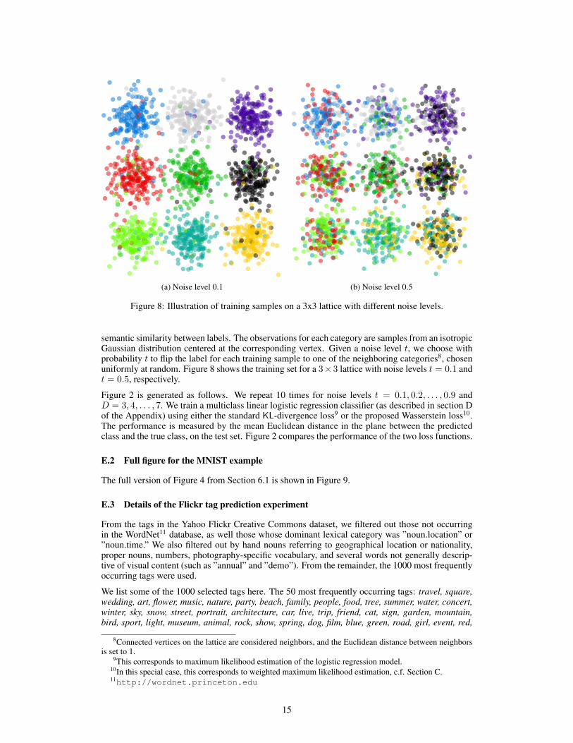
(a) Noise level 0.1 (b) Noise level 0.5

Figure 8: Illustration of training samples on a 3x3 lattice with different noise levels.

semantic similarity between labels. The observations for each category are samples from an isotropicGaussian distribution centered at the corresponding vertex. Given a noise level t, we choose withprobability t to flip the label for each training sample to one of the neighboring categories8, chosenuniformly at random. Figure 8 shows the training set for a 3⇥3 lattice with noise levels t = 0.1 andt = 0.5, respectively.

Figure 2 is generated as follows. We repeat 10 times for noise levels t = 0.1, 0.2, . . . , 0.9 andD = 3, 4, . . . , 7. We train a multiclass linear logistic regression classifier (as described in section Dof the Appendix) using either the standard KL-divergence loss9 or the proposed Wasserstein loss10.The performance is measured by the mean Euclidean distance in the plane between the predictedclass and the true class, on the test set. Figure 2 compares the performance of the two loss functions.

E.2 Full figure for the MNIST example

The full version of Figure 4 from Section 6.1 is shown in Figure 9.

E.3 Details of the Flickr tag prediction experiment

From the tags in the Yahoo Flickr Creative Commons dataset, we filtered out those not occurringin the WordNet11 database, as well those whose dominant lexical category was ”noun.location” or”noun.time.” We also filtered out by hand nouns referring to geographical location or nationality,proper nouns, numbers, photography-specific vocabulary, and several words not generally descrip-tive of visual content (such as ”annual” and ”demo”). From the remainder, the 1000 most frequentlyoccurring tags were used.

We list some of the 1000 selected tags here. The 50 most frequently occurring tags: travel, square,wedding, art, flower, music, nature, party, beach, family, people, food, tree, summer, water, concert,winter, sky, snow, street, portrait, architecture, car, live, trip, friend, cat, sign, garden, mountain,bird, sport, light, museum, animal, rock, show, spring, dog, film, blue, green, road, girl, event, red,

8Connected vertices on the lattice are considered neighbors, and the Euclidean distance between neighborsis set to 1.

9This corresponds to maximum likelihood estimation of the logistic regression model.10In this special case, this corresponds to weighted maximum likelihood estimation, c.f. Section C.11http://wordnet.princeton.edu

15

0 1 2 3 4

p-th norm

0.00

0.05

0.10

0.15

0.20

0.25

0.30

0.35

0.40

Po

ste

rio

rP

ro

ba

bility

0

1

2

3

4

5

6

7

8

9

(a) Posterior prediction for images of digit 0.

0 1 2 3 4

p-th norm

0.00

0.05

0.10

0.15

0.20

0.25

0.30

0.35

0.40

Po

ste

rio

rP

ro

ba

bility

0

1

2

3

4

5

6

7

8

9

(b) Posterior prediction for images of digit 4.

Figure 9: Each curve is the predicted probability for a target digit from models trained with differentp values for the ground metric.

fun, building, new, cloud. . . . and the 50 least frequent tags: arboretum, chick, sightseeing, vineyard,animalia, burlesque, key, flat, whale, swiss, giraffe, floor, peak, contemporary, scooter, society, actor,tomb, fabric, gala, coral, sleeping, lizard, performer, album, body, crew, bathroom, bed, cricket,piano, base, poetry, master, renovation, step, ghost, freight, champion, cartoon, jumping, crochet,gaming, shooting, animation, carving, rocket, infant, drift, hope.

The complete features and labels can also be downloaded from the project website12. We train amulticlass linear logistic regression model with a linear combination of the Wasserstein loss andthe KL divergence-based loss. The Wasserstein loss between the prediction and the normalizedgroundtruth is computed as described in Algorithm 1, using 10 iterations of the Sinkhorn-Knoppalgorithm. Based on inspection of the ground metric matrix, we use p-norm with p = 13, and set� = 50. This ensures that the matrix K is reasonably sparse, enforcing semantic smoothness only ineach local neighborhood. Stochastic gradient descent with a mini-batch size of 100, and momentum0.7 is run for 100,000 iterations to optimize the objective function on the training set. The baselineis trained under the same setting, using only the KL loss function.

To create the dataset with reduced redundancy, for each image in the training set, we compute thepairwise semantic distance for the groundtruth tags, and cluster them into “equivalent” tag-sets witha threshold of semantic distance 1.3. Within each tag-set, one random tag is selected.

Figure 10 shows more test images and predictions randomly picked from the test set.

12http://cbcl.mit.edu/wasserstein/

16

(a) Flickr user tags: zoo, run,mark; our proposals: running,summer, fun; baseline proposals:running, country, lake.

(b) Flickr user tags: travel, ar-chitecture, tourism; our proposals:sky, roof, building; baseline pro-posals: art, sky, beach.

(c) Flickr user tags: spring, race,training; our proposals: road, bike,trail; baseline proposals: dog,surf, bike.

(d) Flickr user tags: family, trip, house; our propos-als: family, girl, green; baseline proposals: woman,tree, family.

(e) Flickr user tags: education, weather, cow, agricul-ture; our proposals: girl, people, animal, play; base-line proposals: concert, statue, pretty, girl.

(f) Flickr user tags: garden, table, gardening; ourproposals: garden, spring, plant; baseline proposals:garden, decoration, plant.

(g) Flickr user tags: nature, bird, rescue; our propos-als: bird, nature, wildlife; baseline proposals: ature,bird, baby.

Figure 10: Examples of images in the Flickr dataset. We show the groundtruth tags and as well astags proposed by our algorithm and baseline.

17