Learning to Sample: Counting with Complex Queries∗

Brett Walenz, Stavros Sintos, Sudeepa Roy, and Jun YangDuke University

Durham, NC, USAbwalenz, ssintos, sudeepa, junyang@cs.duke.edu

ABSTRACTWe study the problem of efficiently estimating counts for queriesinvolving complex filters, such as user-defined functions, or pred-icates involving self-joins and correlated subqueries. For suchqueries, traditional sampling techniques may not be applicable dueto the complexity of the filter preventing sampling over joins, andsampling after the join may not be feasible due to the cost of com-puting the full join. The other natural approach of training andusing an inexpensive classifier to estimate the count instead of theexpensive predicate suffers from the difficulties in training a goodclassifier and giving meaningful confidence intervals. In this paperwe propose a new method of learning to sample where we com-bine the best of both worlds by using sampling in two phases. First,we use samples to learn a probabilistic classifier, and then use theclassifier to design a stratified sampling method to obtain the fi-nal estimates. We theoretically analyze algorithms for obtainingan optimal stratification, and compare our approach with a suite ofnatural alternatives like quantification learning, weighted and strat-ified sampling, and other techniques from the literature. We alsoprovide extensive experiments in diverse use cases using multiplereal and synthetic datasets to evaluate the quality, efficiency, androbustness of our approach.

PVLDB Reference Format:Brett Walenz, Stavros Sintos, Sudeepa Roy, Jun Yang. Learning to Sample:Counting with Complex Queries. PVLDB, 13(3): 389-401, 2019.DOI: https://doi.org/10.14778/3368289.3368302

1. INTRODUCTIONCounting is a fundamental problem in query processing. Count-

ing queries can be expensive to evaluate, especially if it involvestesting a complex predicate to decide whether an object should becounted towards the total. Consider the following example.

∗This work was supported by NSF grants CCF-1513816, CCF-1546392,IIS-1408846, IIS-1552538, IIS-1703431, IIS-1718398, IIS-1814493, NIHgrant 1R01EB025021-01, ARO grant W911NF-15-1-0408, and a GoogleFaculty Award. Any opinions, findings, and conclusions or recommenda-tions expressed in this publication are those of the author(s) and do notnecessarily reflect the views of the funding agencies.

This work is licensed under the Creative Commons Attribution-NonCommercial-NoDerivatives 4.0 International License. To view a copyof this license, visit http://creativecommons.org/licenses/by-nc-nd/4.0/. Forany use beyond those covered by this license, obtain permission by emailinginfo@vldb.org. Copyright is held by the owner/author(s). Publication rightslicensed to the VLDB Endowment.Proceedings of the VLDB Endowment, Vol. 13, No. 3ISSN 2150-8097.DOI: https://doi.org/10.14778/3368289.3368302

EXAMPLE 1 (COUNTING POINTS WITH FEW NEIGHBORS).Suppose table D(id, x, y) stores a set of 2d points, and we wouldlike to count how many points have fewer than k points within dis-tance d from them. We can write the following SQL query:

SELECT COUNT (*) FROM(SELECT o1.id FROM D o1, D o2WHERE SQRT(POWER(o1.x-o2.x,2)+ POWER(o1.y-o2.y,2))<=dGROUP BY o1.id HAVING COUNT (*) <= k);

Here, the objects to be counted are produced by a self-join witha complex condition, followed by GROUP BY and HAVING. This“neighborhood” query has been well studied, with specialized in-dex structures and processing algorithms. Still, there is a goodchance that a typical database system will perform poorly, eitherbecause it has no specialized support for this query type, or it sim-ply fails to recognize this query type from the way the query iswritten. Thus, making such queries run faster can require a lot ofeffort and expertise. There are even more complex cases involv-ing expensive user-defined functions commonly found in machinelearning workloads. The problem we tackle in this paper is how toevaluate counting queries efficiently, and in a general way.

Approximate answers are widely accepted for such expensivecounting queries. Sampling is a powerful technique for producingapproximate answers with statistical guarantees, with a long tradi-tion and active research of its applications in databases. Yet sam-pling for complex queries remains a difficult problem. In general,not all query operators “commute” with sampling. For instance, inExample 1, if we only take a sample of D and evaluate the queryon this sample, it would be difficult to make sense of the result be-cause even the neighbor counts produced by the inner aggregationquery would be off to begin with. Worse, if the predicate involvesa black-box function with table inputs, we cannot expect samplinginput tables to produce usable results.

Still, a viable approach is to conceptually treat the problem ascounting the number of objects satisfying a predicate, where theobjects can be enumerated or sampled efficiently, but the predicateis complex and expensive (e.g., involving user-defined functions orarbitrarily nested subqueries). We would sample some objects forwhich we evaluate the predicate “in full,” and then use these resultsto derive an estimate. For instance, in Example 1, given a point o1from D, the predicate would be a query over (full) D parameterizedby the values of o1.x and o2.x. Of course, evaluating the predicatein full for each sampled object can be expensive, but evaluating theoriginal query as a whole can be much worse—there may be nobetter way for the database systems to process this query than anested-loop join. While this sampling-based approach is simpleand general, a question is whether we can make it more efficient.

Machine learning is another natural approach to this problem.It has the potential of being more “sample-efficient” because of

390

its ability to generalize to unseen objects. One could draw somesamples, pay the cost to “label” them (i.e., evaluate the expensivepredicate), and use the labeled samples to learn a cheap classi-fier that approximates the result of the expensive predicate. Thelearned classifier can then be applied to objects to obtain an esti-mated count. Beyond this naive approach, we can apply ideas fromquantification learning [6]. However, some difficulties remain: it ishard to offer meaningful statistical guarantees (such as confidenceintervals provided by sampling), and training a good classifier canbe difficult and tricky itself (e.g., with challenges such as featureand model selection as well as overfitting).

A natural question is whether we can combine learning and sam-pling to get the “best of both worlds”: we want the ability to gener-alize by learning, but at the same time we want the statistical guar-antees offered by sampling. This paper answers this question inpositive. One idea is to use sampling to assess the errors producedby the learned classifier and correct its estimated count. We alsoprovide a novel alternative that “learns to sample.” The key ideahere is not to rely directly on the learned classifier’s predictions,but instead exploit the classifier’s knowledge in a more controlledmanner by using it to design a sampling scheme. Then, we applythe sampling scheme to derive our estimates, complete with statis-tical guarantees. A good classifier leads to an efficient samplingscheme that uses few samples to get low-variance estimates; on theother hand, a poor classifier can lead to a less efficient samplingscheme that needs more samples to achieve the same accuracy, butwe will always have unbiased estimates with confidence intervals.

Specifically, we make use of the scores produced by classifiersthat reflect how confident they are in their predictions. Such scoresare readily available for popular classification methods in standardlibraries. A straightforward method is learned weighted sampling,which assigns higher sampling probabilities to objects that are moreconfidently predicted to contribute to the result count. This methodis still sensitive to the scores produced by the classifiers, and tendsto focus more on confidently positive objects instead of uncertainobjects—but arguably, uncertain objects intuitively provide moreinformation when labeled.

Hence, we further propose learned stratified sampling, which re-lies even less on the quality of the classifier. Instead of using thevalues of the scores, we use the scores only to induce an order-ing among the objects. Based on this ordering, and with help fromsome additional samples, we find the optimal stratified samplingdesign that jointly considers the partitioning of objects into strataand the allocation of additional samples across strata. The score-induced ordering is useful because it brings together objects withsimilar levels of uncertainty, and in particular encourages puttingthe certainly positive objects and certainly negative objects intoseparate strata with low within-stratum variances. The samplingdesign problem is challenging because of joint consideration ofstratification and allocation; we propose algorithms for this opti-mization problem with trade-offs between speed and optimality.

Our experiments show that our learn-to-sample approach gener-ally outperforms approaches that are based on either sampling orlearning alone, or those that apply sampling only to error assess-ment and correction. We achieve unbiased estimates with lowervariances than other approaches, and in practice, the overhead oflearning and sampling design is negligible compared with the to-tal cost of evaluating expensive predicates on samples. Moreover,learned stratified sampling delivers robust performance even withpoor classifiers. Finally, a key practical advantage of our learn-to-sample approach is that it is easy to implement: its constituentlearning and sampling components are available off-the-shelf, sowe readily benefit from both the classic sampling literature and a

growing toolbox of classification algorithms. For example, for ourexperiments, we were able to apply standard classification algo-rithms out-of-box with very little tuning, thanks to the robustnessof the learn-to-sample approach.

2. PROBLEM DEFINITIONConsider a set of objects O, and a Boolean predicate q : O →0, 1, where 1 denotes true. We say an object o is positive ifq(o) = 1, or negative if q(o) = 0. Our goal is to estimate C(O, q),the number of positive objects in O; i.e., C(O, q) =

∑o∈O q(o).

In general, each object o can have a complex structure (with mul-tiple attributes including set-valued ones), and q(o) can be arbitrar-ily complex (e.g., accessing related information beyond the con-tents of o, comparing o with other objects in O, etc.).

We make two assumptions: 1) evaluation of q is costly; 2) mem-bers of O can be efficiently enumerated. The terms “costly” and“efficient,” of course, are relative. While the techniques in this pa-per do not depend on these assumptions for correctness, our pro-posed approach is intended for situations where these assumptionshold. For example, a costly q would make it attractive to use sam-pling to avoid evaluating q for all objects, or to use a learned modelthat predicts the outcome of q at a lower cost.

It should be obvious that the problem formulation above han-dles single-table selection queries whose conditions potentially in-volve expensive user-defined functions. The problem formulationis also general enough to capture more complex queries. The firstexample below illustrates the case where q is a complex SQL con-dition involving an aggregate subquery; the second illustrates thecase where q involves a black-box function.

EXAMPLE 2 (k-SKYBAND SIZE). Consider a set of 2d pointsin table D(id, x, y). A point p1 dominates another point p2 if p1’sx and y values are (resp.) no less than those of p2 (i.e., p1.x ≥p2.x ∧ p1.y ≥ p2.y), and at least one of them is strictly greater(i.e., p1.x > p2.x∨ p1.y > p2.y). The so-called k-skyband for thepoint set D is the subset of points that are dominated by fewer thank others. Given o ∈ D, we define q(o) to test its membership in thek-skyband using the following SQL condition:(SELECT COUNT (*) FROM DWHERE x >= o.x AND y >= o.y AND (x>o.x OR y>o.y)) < k

Note that this predicate involves an aggregate subquery parame-terized by o. The number of points in the k-skyband is then thenumber of points satisfying q. Here, object enumeration is efficient(just scan D), while predicate evaluation is costly in comparison(without specialized indexes).

Alternatively, we can write the whole k-skyband size query usinga self-join and nested aggregation, without explicitly referring to q:SELECT COUNT (*) FROM(SELECT o1.id FROM D o1, D o2WHERE o2.x >= o1.x AND o2y >= o1.y

AND (o2.x > o1.x OR o2.y > o1.y)GROUP BY o1.id HAVING COUNT (*) < k);

EXAMPLE 3 (RELEVANT DOCUMENT COUNT). Consider aset of documents in table D(id, text). Each document, based onthe content of its text, can be associated with zero or more labelsfrom a predefined set of labels of interest. For example, during elec-tronic discovery for a legal proceeding, D can be a set of emails anddocuments, and one such label may indicate whether a document isin support of or against a particular action. Let labels(text) de-note a function that examines a document and returns the subset oflabels that it is associated with. We mark a document as highly rel-evant if it is associated with at least k labels. The following queryreturns the number of highly relevant documents:

391

SELECT COUNT (*) FROM D oWHERE len(labels(o.text)) >= k;

Here, q is the WHERE predicate, but it involves a complex black-box function labels whose evaluation can be very expensive. Forexample, if labels are highly specialized for a given proceeding,there may not exist good automated labeling procedures and wewould have to evaluate labels manually. In general, the predicatethat determines whether a document is relevant can be even morecomplicated than counting how many labels it is associated with,but our problem formulation and solutions are designed to workwith arbitrarily complicated q.

Handling More General SQL Queries An observant reader willnotice the similarity between the last query in Example 2 and theone counting points with few neighbors in Example 1. Despite thelatter query’s lack of an explicit per-object predicate, it is not hardto see that we can define q(o) for o ∈ D as the following com-plex SQL condition involving an aggregate subquery (analogous toExample 2 above):

(SELECT COUNT (*) FROM DWHERE SQRT(POWER(o.x-x,2)+ POWER(o.y-y,2)) <= d) <= k

More generally, suppose we are interested in counting the num-ber of results for the following SQL aggregate query:

SELECT E FROM L,R -- (Q1)WHERE θL AND θLR

GROUP BY GL HAVING φ;

In the above, GL is the list of group by columns, L denotes the listof tables with columns in GL, and R denotes the list of other tablesin the join with no group-by columns; θL refers to the part of theWHERE condition that be evaluated over L alone, θLR refers to theremaining part of the WHERE condition, and φ refers to the HAVINGcondition; finally, E is the list of output expressions for each group.The problem of counting the number of results can be formulatedby defining the set O of objects as:

SELECT DISTINCT GL FROM L WHERE θL; -- (Q2)

and the predicate q(o) as:

EXISTS(SELECT GL FROM L, R -- (Q3)WHERE θLR AND GL=o.*GROUP BY GL HAVING φ)

Again, the key takeaway is that our problem formulation is generalenough to support complex queries involving joins and aggregates(besides the final counting). Our approach works well as long asthe set of objects is cheap to enumerate (i.e., the local selection θLin (Q2) is easy to evaluate), while the per-object predicate (Q3) isrelatively more expensive (which is usually the case because of joinand aggregation).

3. BASELINE METHODSWe present a number baseline methods for estimating C(O, q).

While these methods are not new, we note that some connections toour problem (e.g., quantification learning and sampling-based datacleaning) have never been made explicit or evaluated previously.

3.1 Sampling-Based MethodsSimple Random Sampling (SRS) The problem of estimatingC(O, q) using sampling has been studied extensively in the con-text of estimating proportions [24]. A straightforward method issimple random sampling (SRS). Let S ⊆ O denote the set of nobjects drawn randomly without replacement from the set O of all

N objects. For each o ∈ S, we evaluate q(o). Then, an unbi-ased estimator of C(O, q) is pN , where the estimated proportionp = 1

n

∑o∈S q(o). There are a number of ways to derive a confi-

dence interval for this estimation. The most popular one is the Waldinterval, which approximates the error distribution using a normaldistribution: the (1− α) confidence interval for p in this case is

p± zα/2√

p(1−p)n· N−nN−1

.

The usual caveats apply: if q is highly selective or highly non-selective, the Wald interval is unreliable because normal distribu-tion approximation fails; one can use the more reliable Wilson in-terval instead. See standard sampling literature [24] for details.Stratified Sampling (SSP and SSN) Stratified sampling is amethod that works especially well when the overall population canbe divided into subpopulations (strata) where objects are homoge-neous within each stratum. For example, if there is a way to divideO into two strata where one contains mostly positive objects andthe other contains mostly negative objects, we can sample the twostrata independently and use much fewer samples overall than SRSto achieve the same confidence interval. The problem, of course, isthat we do not know the outcome of each q(o) unless we first eval-uate it. A practical solution is to choose some attributes of o whosevalues are readily available and likely correlated with the outcomeof q(o); we can then stratify O according to these surrogates. Inour case, a natural choice for surrogates would be the attributes ofo used in computing q(o); e.g., for Example 1, we would choose xand y and grid the 2d space into the desired number of strata.

Suppose we are given a partitioning of O into H strata O1,O2,. . . ,OH , where Nh = |Oh| denotes the size of each stratumh, and an allocation of samples n1, n2, . . . , nH , where nh is thenumber of samples allotted to stratum h. Stratified sampling ran-domly draws the allotted number of samples from each stratum;denote these samples by S = ∪Hh=1Sh, where nh = |Sh|. Foreach stratum h, using Sh, we can derive an unbiased estimatorfor the proportion ph of positive objects therein (as described forSRS above). Then, an unbiased estimator of C(O, q) is pN ,where p =

∑Hh=1 Whph is the estimated overall proportion and

Wh = Nh/N is the weight of stratum h. The variance in p is

Var(p) =∑Hh=1

W2hS

2h

nh− 1

N

∑Hh=1 WhS

2h, (1)

where Sh is the standard deviation of stratum h (i.e., of the mul-tiset q(o) | o ∈ Oh). The (1 − α) confidence interval for p isp± tα/2

√Var(p),n where Var(p) is an unbiased estimate of Var(p)

computed using (1) with S2h substituted by an unbiased estimate

from Sh. See standard sampling literature [24] for details.A simple strategy is proportional allocation, where the number

of samples allotted to each stratum is proportional to its size, i.e.,nh ∝ Nh. We refer to stratified sampling with proportional alloca-tion as SSP. A more sophisticated alternative, Neyman allocation,optimally allocates samples according to nh ∝ NhSh, which min-imizes Var(p). We refer to this alternative as SSN. In practice, aswe do not know Sh in advance, SSN proceeds in two stages:

1. Randomly draw a set SI of samples to evaluate q with, anduse them to derive an estimate of Sh for each stratum h. Thencalculate the Neyman allocation using these estimates.1

2. Randomly draw the allotted number of samples from eachstratum.

1Standard caveats apply: given the desired total number of samples, weensure that no stratum is allotted more samples than it contains, and thatno stratum is allotted fewer than a prescribed minimum number of sam-ples (even if its estimated standard deviation is close to 0); we do so byrebalancing the allocation after meeting these constraints.

392

3.2 Learning-Based MethodsSince q is expensive to evaluate, it is natural to consider learning

a binary classifier f : O → 0, 1 to approximate the behavior ofq. We can draw a random sample S from O, evaluate q on them toobtain the ground truth, and then use the results to train the classi-fier. The classic classification problem strives to classify each inputobject correctly, but for our problem, we are concerned only withthe number of objects whose ground-truth labels are 1. The result-ing problem is an instance of quantification learning [6], whosegoal is to estimate the class distribution as opposed to individuallabels. While specialized algorithms are possible, it is appealing toadapt classic classification algorithms for quantification learning,thereby leveraging a rich palette of mature techniques. In this sec-tion, we first explore how, given a classifier f that approximates q,we can use quantification learning to estimate C(O, q).

We will not delve into specific classification algorithms here, be-cause they are not this paper’s focus; our methods can work withany of them. For feature selection, we use a simple heuristic thatselects the attributes of o referenced in q, e.g., columns of L refer-enced by θLR in (Q1) (Section 2). We also note that training can beimproved by active learning [6]; for additional discussion, pleasesee the full version of this paper [25].

Classify-and-Count (QLCC) A straightforward and natural ap-proach is Classify-and-Count [6], which we refer to as QLCC.Suppose we randomly select S ⊆ O as training data and letCS = C(S, q) denote the count of positive objects therein. Af-ter learning f from S, we evaluate f(o) for each “test object”o ∈ O\S. Let Cobs =

∑o∈O\S f(o) denote the “observed count”

of f over the test data. We simply return Cobs + CS as the esti-mate for C(O, q). Should the classifier be accurate over the testdata, this estimate will be accurate as well. However, it should beclear that QLCC is susceptible to classification errors and can pro-duce wildly skewed estimates when false positive/negative countsare imbalanced.

Adjusted Count (QLAC) To mitigate this problem, a recom-mended approach is Adjusted Count [6], which we refer to asQLAC. The basic idea is to further adjustCobs using the rates of trueand false positives estimated empirically from the training data. Inmore detail, we use k-fold cross validation on the samples S tocompute tpr and fpr , the estimated true and false positive rates,respectively. Then, we obtain an “adjusted count” Cadj of f overthe test data by adjusting the observed count Cobs as follows2:

Cadj =Cobs − fpr · |O\S|

tpr − fpr. (2)

Finally, we return Cadj + CS as the estimate for C(O, q).

3.3 Learning with Sample-based CorrectionOne idea for combining learning and sampling is to follow

QLCC (Classify-and-Count) with another phase, where we ran-domly sample additional objects, evaluate q on them, assess theerrors in the learned classifier f , and correct the result of Classify-and-Count accordingly. We call this method QLSC, for “quantifi-cation learning with SampleClean,” as it is inspired by the work

2To see why, note that the proportion p of “observed positive” objects in thetest data can be computed by p = p·tpr+(1−p)·fpr , where p denotes theactual positive proportion, and tpr and fpr are the true and false positiverates. We can solve for p, and note that multiplying p and p by the size ofthe test data yields the observed and actual counts. Replacing tpr and fprwith their estimates then gives us (2).

of [26] on using sampling for data cleaning.3 More precisely, recallthat QLCC samples S ⊂ O, learns f , and estimates the positivecount over remaining objects as Cobs =

∑o∈O\S f(o). QLSC

then proceeds with drawing (uniformly at random) another set S ′of objects from O \ S, and for each o ∈ S ′ computes the errorf(o) − q(o). The average error ε over S ′ gives an unbiased esti-mator for the average error overO \S, so we can correct the countover O \ S as Cobs − ε|O \ S|. Adding CS (positive count in S)yields the overall estimate. Confidence intervals can be derived asin Section 3.1 because the second phase of QLSC is basically SRS.

QLSC is similar to QLAC (Section 3.2) in that both seek to cor-rect the result of QLCC by assessing its errors on labeled samples.However, QLAC produces only a point estimate while QLSC canprovide confidence intervals.

4. LEARNING-TO-SAMPLE METHODSIn the previous section, we have seen how sampling and learning

can be applied to problem of estimating C(O, q). Learning is at-tractive for its ability to “generalize” knowledge of q to unsampledobjects, but it does not offer the guarantees provided by sampling(e.g., confidence intervals), and its accuracy depends heavily onthe quality of the classifier it learns. A natural question is whetherwe can combine learning and sampling to get the “best of bothworlds.” QLSC (Section 3.3) represents a baseline approach to-wards this goal: it uses sampling to correct the count predicted bythe classifier, but its sampling scheme does not take advantage ofthe learned model in any way, and a poor classifier would result ina poor starting point.

This section proposes two methods that combine learning andsampling more effectively. Both methods proceed in two phases.The first phase is learning, and is identical for the two methods:we randomly sample objects, evaluate q on them, and train a binaryclassifier, as we did in Section 3.2. However, we are not going touse this classifier to get a count (as a starting point or otherwise).Instead, we assume that the classifier provides a scoring functiong : O → [0, 1]: if g(o) = 1 (or 0), the classifier is totally confidentin predicting q(o) to be 1 (or 0, resp.); a value strictly between 0 and1, on the other hand, indicates uncertainty (e.g., 0.5 means a toss-up). For some classifiers (e.g., random forest), one can intuitivelyinterpret g(o) as the probability that q(o) = 1, but in general, g(o)may not have a probabilistic interpretation. Regardless, the scoringfunction g gives us a way to gauge the certainty in the predictedlabels. We assume that, compared with q, g is cheap to evaluate (inpractice it is often a byproduct of classification).

The second phase is sampling, but differs between the two meth-ods. The first method, Learned Weighted Sampling (LWS), is themore straightforward one of the two. Treating g(o) has a guess ofhow much each object o contributes to C(O, q), LWS samples ob-jects with higher g(o) with higher probability. The second method,Learned Stratified Sampling (LSS), uses g to guide the partition-ing of objects into strata, with the goal of reducing the variance ofestimates using stratified sampling.

3While SampleClean [26] deals with the different problem of evaluatingaggregates over dirty data, its techniques can be adapted to our quantifi-cation learning setting by conceptually regarding the labels produced bythe learned classifier as dirty data; “cleaning” a dirty label involves sam-pling the object and paying the cost of evaluating q. Specifically, QLSCcorresponds to their NormalizedSC technique, which corrects the aggregateresult computed over dirty data using the errors observed on data randomlyselected for cleaning. Their RawSC technique, which randomly cleans dataand estimates the result from only the cleaned labels, basically correspondsto the sampling-based baseline methods in our Section 3.1.

393

The novelty of these two methods lies in their use of learning toinform sampling. Thanks to sampling, we still get accuracy guar-antees in the form of confidence intervals. At the same time, we getthe benefit of learning without relying on it for correctness. A goodclassifier leads to more efficient sampling designs; on the otherhand, a poor classifier leads to a less efficient sampling design, butwe still have unbiased estimates with confidence intervals. As wewill see, between the two methods, LSS is even more robust andless dependent on the quality of the learned classifier than LWS.

The remainder of this section describes the second phase forthese two methods in detail. Let SL denote the samples used inthe first phase for learning a classifier with scoring function g. Wenow focus on estimating C(O \ SL, q) in the second phase. In thefollowing, we will abuse notation for simplicity: we shall refer toO \ SL simply as O instead, and let N = |O|.

4.1 Learned Weighted SamplingThe second phase of LWS can be seen as a form of probability-

proportional-to-size (PPS). In general, PPS relies on a “size mea-sure” that is believed to be correlated to the variable of interest.Objects with large size measures are deemed more important in es-timation; hence, objects are drawn with probabilities proportionalto their size measures. In our case, the variable of interest is theresult of q(o), so the learned g(o) can serve as the size measure.However, to guard against an overconfident (and potentially inaccu-rate) classifier, we adjust the sampling probabilities so every o hassome chance of being sampled (even if g(o) = 0). Specifically, weassign each o an initial sampling probability π(o) ∝ max(g(o), ε),where ε > 0 is a (small) prescribed threshold. We then sampleobjects from O according to π without replacement, evaluate q onthe sampled objects, and estimate C(O, q).

There are a number of estimators available from the litera-ture [14], including the popular Horvitz-Thompson estimator. Weuse the Des Raj estimator, whose calculation is simpler and canprovide “ordered” estimates, i.e., running estimates of mean andvariance as samples are being drawn. Let o1, o2, o3 . . . denote thesequence of objects drawn according to π without replacement.We compute the following quantity after drawing each oi (with thesummations below yielding 0 in case of i = 1):

pi = 1N

(∑i−1j=1 q(oj) + q(oi)

π(oi)

(1−

∑i−1j=1 π(oj)

)). (3)

The estimate for C(O, q) after drawing the n-th sampled objectwould be p(n)N , where the estimated proportion p(n) of positiveobjects is simply the average of all pi’s so far:

p(n) = 1n

∑ni=1 pi.

And the variance in p(n) can be estimated as follows:

Var(p(n)) = 1n(n−1)

∑ni=1(pi − p(n))2.

LWS is very efficient when the learned classifier is accurate andconfident. To see why, suppose the true proportion of positive ob-jects in O is p. For an accurate and confident classifier, assum-ing an arbitrarily small ε, π(o) would be arbitrarily close to 0 ifq(o) = 0, or 1

pNotherwise. Therefore, each sampled object oi will

have q(oi) = 1 and π(oi) = 1pN

. Plugging these into (3) and sim-plifying the equation yields pi = p for all i, so the estimate p(i) atevery step will be perfectly accurate.

On the other hand, LWS’s efficiency can suffer with a poor clas-sifier. Even though it still produces unbiased estimates (regardlessof the choices of π(o)’s), it may require many more samples toachieve a tight confidence interval if it gets the priorities wrong.

Another indication that LWS may not be best for our setting isits preference for objects with high g(o). Intuitively, focusing in-stead on objects with g(o) in the toss-up range reveals more infor-mation. Note that traditionally, PPS applies to the more generalsetting where the variable of interest can be of any value; hence, itis natural to focus on objects with potentially higher contributionto the result. In our setting, however, the value of interest, q(o), iseither 0 or 1. This limited range makes our problem easier, as wedo not need to worry about cases where inclusion or exclusion ofobjects with extremely high values can seriously impact the esti-mates. At the same time, this more constrained setting also enablesthe possibility for better sampling designs, which we explore next.

4.2 Learned Stratified SamplingAs discussed in Section 4.1, the quality of the learned classifier

can adversely impact the efficiency of LWS, because the values ofscoring function g directly control the sampling probabilities. Wenow present LSS, which uses g more conservatively, and in a waythat naturally encourages exploration of uncertain outcomes (as op-posed to certain positives).

Following the learning phase, LSS conceptually sorts the objectsin O by g (say, in increasing score order). At a high level, LSSapplies stratified sampling to O, where stratification is done ac-cording to this ordering; i.e., each stratum covers objects whose gscores fall into a consecutive range. More specifically, the secondphase of LSS proceeds in two stages:

1. Randomly draw SI ⊆ O to evaluate q, and use the resultsto design a sampling scheme for the second stage—namely,the partitioning of O into strata as well as an allocation ofsecond-stage samples among these strata.

2. Randomly draw SII ⊆ O \ SI to evaluate q, according tothe sampling scheme designed by the first stage, and use theresults to estimate C(O, q).

Several points are worth noting:(Versus LWS) While LWS uses the actual g values in its sampling

design, LSS uses only the ordering of g values among ob-jects. Hence, LSS relies less on the learned classifier. Wewill validate this observation with experiments in Section 5.On the other hand, the ordering induced by g is useful toLSS because it intuitively brings together objects with simi-lar levels of uncertainty, and in particular encourages puttingthe confidently positive objects and confidently negative ob-jects into separate strata with low within-stratum variances.

(Versus Basic Stratified Sampling) While the second phase of LSSuses stratified sampling, this phase differs from the baselinemethods in Section 3.1 in important ways: (i) stratificationin LSS is based on the learned g instead of surrogate objectattributes; (ii) LSS uses SI to jointly design stratification andallocation; in contrast, SSN only uses SI to design allocation(given stratification), while SSP does not have a first stage.

(Samples in Learning and Sampling Phases) The samples wedraw in the sampling phase of LSS (SI ∪ SII above) areseparate from those drawn in the learning phase. Since thesamples from the learning phase already affect (through thelearned g) the ordering of O for stratification, we choose touse new, independent samples (SI) for sampling design inorder to minimize reliance on the classifier quality.4

The remainder of this section discusses how we design the sam-pling scheme for the second stage in detail. Formally, we de-fine the design problem as follows. Consider an ordered set Oof objects o1, o2, . . . , oN ordered by g with ties broken arbitrarily,4As future work, it would be interesting to investigate safe reuse of samplesfrom the learning phase in less conservative ways.

394

which can be efficiently computed as we assume that the classifieris easy to execute. A stratification of O into H strata, specifiedby (N1, N2, . . . , NH) where

∑Hh=1 Nh = N , defines the parti-

tioning of O into subsets O1,O2, . . . ,OH . Here O1 includes ob-jects with indices ≤ N1, and Oh, h ≥ 2 denotes the subset of ob-jects whose indices fall within the interval (

∑h−1j=1 Nj ,

∑hj=1 Nj ].

Recall from Section 3.1 that (1) gives the variance in the esti-mator of C(O, q)/N for stratified sampling, given the stratifica-tion (N1, N2, . . . , NH) and a sample allocation (n1, n2, . . . , nH)where we draw nh objects fromOh. However, we do not know theSh terms in (1) in advance, since they denote the standard deviationof the actual q(oi) values of the objects oi ∈ Oh that are expen-sive to compute, so LSS instead seeks to minimize the variance ofC(O, q) given by (1) estimated using the first-stage samples SI.

More precisely, suppose the first-stage sample SI consists of mobjects oı1 , oı2 , . . . , oım where 1 ≤ ı1 < ı2 < · · · < ım ≤N . We aim to find a stratification (N1, N2, . . . , NH) to minimizethe objective given in (5) below that estimates the variance in theestimator of C(O, q) using n samples in total in the second stage.Here we assume SI

h = Oh ∩ SI, mh = |SIh|, nh is number of

second-stage samples in Oh,∑Hh=1 nh = n, and the variances S2

h

using the first-stage samples SI are estimated as

s2h = 1

mh−1

∑o∈SI

h(q(o)− C(SI

h, q)/mh)2. (4)

Then the variance of the estimated C(O, q) obtained by simplify-ing (1) is given by:

V (N1, N2, . . . , NH) =∑Hh=1

N2hs

2h

nh−∑Hh=1 Nhs

2h. (5)

The remainder of this section describes our algorithms for com-puting the optimal stratification given SI. Note that the optimalityof stratification depends on the allocation strategy used. We firstpresent the case of using Neyman allocation, which minimizes thevariance for a given stratification. In this case, LSS gives the over-all optimal sampling design that jointly considers stratification andallocation. Then, we briefly discuss the case of proportional alloca-tion, which is simpler but not optimal for a given stratification. Inthis case, we would find the stratification that makes proportionalallocation most effective; the optimization problem is much easierthan the case of Neyman allocation.

Optimizing the StratificationRecall from Section 3.1 that under Neyman allocation using SI,nh = n(Nhsh)/(

∑Hh=1 Nhsh). Hence, we can further sim-

plify (5), the minimization objective, as follows:

V (N1, N2, . . . , NH) = 1n

(∑Hh=1 Nhsh

)2

−∑Hh=1 Nhs

2h. (6)

A naive algorithm would compute V for all possible stratifications(N1, N2, . . . , NH) and pick the best, but the number of possibili-ties is Ω(NH), and computing V involves going over SI, which isexpensive even for small number of partitions (e.g., when H = 3).

Before presenting our algorithms, we describe some ideas usefulto combat these challenges. First, note that in the expression for Vin (6), from (4), the sh terms depend only on the subset of objectsSIh sampled in SI in each stratum h, and the precise locations of

stratum boundaries between these sampled points only affect theNh terms. This observation suggests that we may be able to firstconsider the partitioning of SI among strata, and then decide whereprecisely the stratum boundaries lie amongO. Later in this section,we will start with an algorithm that uses this strategy, where giventhe partitioning of SI, the optimal Nh’s can be solved directly and(almost) exactly in the case of H = 3. Building on the insights re-vealed in this simple case, we then present two general algorithms

for any H providing different trade-offs between speed and accu-racy. Both of these algorithms tame complexity by restricting thepotential locations of the stratum boundaries.

Second, we can speed up the computation of V significantly us-ing precomputation. By sorting the m objects in SI by g, we cancompute a prefix-sum index Γ, such that Γ(k) =

∑k=1 q(oı) (for

1 ≤ k ≤ m) returns the number of positive objects among the firstk objects in SI. To obtain the indices of sampled objects within theordered O (i.e., ı1, . . . , ım), there is no need to sort all objects inO by g. Instead, note that the m objects in SI divide the range ofg values into m+ 1 buckets; we can simply make one pass overOand maintain the count of objects whose g values fall within eachbucket. After the pass overO completes, we scan the bucket countsto determine ı1, . . . , ım.• DirSol (an almost optimal stratification forH = 3H = 3H = 3): Here we

try all pairs of SI as possible rough boundaries. In particular,for each pair of consecutive samples as per g, we assume that thefirst element is the last sampled object in the first strata, while thesecond element is the first sampled object in the third strata. Inorder to find the exact boundaries in O, we formulate and solvean optimization problem.• LogBdr (an approximate stratification for anyHHH , generaliz-

ing DirSol): It considers all possible ways of partitioning the msampled objects in SI among H strata generalizing the ideas inDirSol. Unlike DirSol, however, for each such partitioning, wedo not attempt to solve directly for the actual stratum boundarieswithin O; instead, we consider only a set of candidate boundaryindices, chosen judiciously to ensure that we can still find a rea-sonably good solution. In particular, between two consecutiveobjects oık and oık+1 in SI (with respect to g), we consider theobjects in O that are 2i apart from oık as boundary indices.• DynPgm (a dynamic-programming-based algorithm for anyHHH , faster than LogBdr but with worse approximation guar-antees): A straightforward application of dynamic programmingdoes not work since the objective in (6) is non-separable. Toovercome this difficulty, we isolate the non-separable term inthe objective function and solve a suite of dynamic programswhere each of them operates under a different upper bound onthe non-separable term. In order to improve the running time,we only consider as possible boundaries the set SI and the addi-tional boundary indices similar to DirSol. In the end, we returnthe best result over the dynamic programs (details in [25]).• DynPgmP (222-approximation for proportional allocation):

Recall from Section 3.1 that under proportional allocation,nh = nNh/N . Hence, we can further simplify (5) toV (N1, . . . , NH) = N−n

n

∑Hh=1 Nhs

2h. The objective is much

simpler than the objective for Neyman allocation and the result-ing optimization problem is indeed separable, so it can be solvedreadily by dynamic programming. To improve the efficiency, weuse the same idea as in LogBdr and DynPgm with additionalboundary indices (details in [25]).

In addition to optimizing the objective in (6), we impose the fol-lowing constraints for each stratum h: For two chosen thresholdsNt and mt, (i) Nh ≥ Nt, i.e., each stratum is large enough, and(ii) mh ≥ mt, i.e., the stratum contains enough first-stage samplessuch that sh is a reasonable variance estimate. In practice, we haveset mt to be around 5 and Nt larger.

DirSol: We now give more details on DirSol. For H = 3, weneed to pick two boundaries separating strata O1, O2, O3. To thisend, suppose the last sampled object (with the largest g value) inO1 is the i-th object in SI, and the first sampled object (with thesmallest g value) in O3 is the j-th object in SI. The algorithm

395

considers every possible (i, j) pair where mt ≤ i < i+mt < j ≤m−mt + 1.

Given oıi as the last sampled object in O1 and oıj asthe first sampled object in O3, we can readily computes1, s2, s3 in (6) using the precomputed index Γ: s2

1 =Γ(i)i−1

(1− Γ(i)

i

), s2

2 = Γ(j−1)−Γ(i)j−i−2

(1−Γ(j−1)−Γ(i)

j−i−1

), and s2

3 =

Γ(m)−Γ(j−1)m−j

(1−Γ(m)−Γ(j−1)

m−j+1

).

Then, noting that N2 = N − N1 − N3, we can writeV (N1, N2, N3) as bivariate quadratic function f(N1, N3) of theform a1N

21 +a2N

23 +a3N1N3 +a4N1 +a5N3 +a6, where coeffi-

cients a1, . . . , a6 are computed from s1, s2, s3, n, and N (see [25]for detailed derivation). Our goal is to minimize f(N1, N3) subjectto the following constraints:• maxNt, ıi ≤ N1 ≤ ıi+1 − 1; i.e., the last sampled object

in O1 is indeed the i-th one in SI, and |O1| ≥ Nt.• maxNt, N − ıj + 1 ≤ N3 ≤ N − ıj−1; i.e., the first

sampled object in O3 is the j-th in SI, and |O3| ≥ Nt.• N1 +N3 ≤ N −Nt; i.e., |O2| ≥ Nt.

These constrains define a 2-dimensional polygon R with at most5 sides. We optimize the function f over R using a standard al-gebraic method by considering (i) the critical points of f , and (ii)the boundary of R. We repeat the above procedure for each pairof sampled objects, and in the end return the stratification with theoverall minimum variance (see [25] for additional details and thepseudocode). We call this algorithm DirSol (for direct solve). Thefollowing theorem summarizes its time complexity and accuracy.

THEOREM 1. Given an ordered set O of N objects and a sam-pled subset SI of m objects, let v∗ denote the minimum value ofestimated variance defined in (6) achievable using n samples un-der stratified sampling with H = 3 strata where each stratumcontains at least Nt objects. Assuming Nt > n, DirSol runs inO(N logm + m2) time and finds a stratification resulting in esti-mated variance v ≤ (1 + 2

Nt+ 2

Nt−n + 4Nt(Nt−n)

)v∗.

Note the assumption of Nt > n above; without it, the approxi-mation factor would be arbitrarily bad. In practice, however, thisassumption is weak and often holds in practice: e.g., if we take a5% sample of O in the second stage, this assumption means thateach stratum in O contains at least 5% of O.LogBdr: Given a partitioning of the sampled objects, considertwo consecutive sampled objects oık and oık+1 that are put intodifferent strata (there are H − 1 such pairs of objects). When de-ciding where exactly to draw the boundary between oık and oık+1 ,the algorithm only considers the set Bk of candidate boundary in-dices ık, ık + 20, ık + 21, ık + 22, . . . up to (but not including)ık+1; we also add ık+1 − 1 if it is not already in Bk. Choosing aparticular index i from Bk means the stratum containing oık endswith oi. Then we simply check all candidate stratifications formedby choosing one index from each of the H − 1 sets of candidateboundary indices. We call this algorithm LogBdr (for logarithmicnumber of candidate boundary indices). Theorem 2 summarizes itstime complexity and accuracy (proof is in [25], the approximationfactor can be improved if we increase the running time).

THEOREM 2. Given an ordered set O of N objects and a sam-pled subset SI of m objects, let v∗ denote the minimum value ofestimated variance defined in (6) achievable using n samples un-der stratified sampling with H strata where each stratum containsat least Nt objects. Let N∗h denote the size of stratum h in this op-timum solution. Assuming Nt > n, LogBdr runs in O(N logm +HmH−1 logH−1 N) time and finds a stratification resulting in es-timated variance v ≤ max4, 2 + 2 max1≤h≤H

N∗hN∗

h−nv

∗.

5. EXPERIMENTSMost of our experiments are based on three scenarios, each with

its own real-world dataset and counting query template:(Sports) The data contains yearly performance statistics for play-

ers in the Major League Baseball. We focus on pitchingstatistics, which exclude a portion of the players. We con-sider the k-skyband size query in Example 2, where eachpoint is a player-year combination (there are about 47,000 ofthem), and x and y refer to runs and home runs.

(Neighbors) The data comes from KDD Cup 1999, where the goalwas to learn a predictive model that could distinguish legiti-mate and illegitimate (intrusion attacks) connections to a ma-chine. The original dataset contains 4.9 million records with41 features and a binary label. We removed many sparserows, resulting in 73,000 points. We consider the query inExample 1 that counts points with few neighbors.

(Text) We consider the relevant document count query in Ex-ample 3. Since we do not want to manually evaluatethe predicate ourselves in experiments, we use the LSHTCdataset [23], which provides ground-truth labels (Wikipediacategorization) for 2.4M documents from Wikipedia. Thesame dataset was used in [18]. In our experiments, each al-gorithm is charged a cost for revealing the true label, whichin practice would be expensive.

To experiment with different selectivities of the predicate q, we ad-just query parameter settings (k for Sports; k and d for Neighbors;k for Text). We also create synthetic datasets based on Sports tostudy how data distributions affect learned models and the perfor-mance of various algorithms; for details see Section 5.2.

We compare the following algorithms:• Sampling-based (Section 3.1): simple random sampling

(SRS) and stratified sampling (SSP, with proportional allo-cation, and SSN, with Neyman allocation in two stages). Forstratified sampling (which applies to Neighbors and Sportsbut not to Text), we use attributes x and y as surrogates; eachstratum is a rectangle in the 2d x-y space. Unless otherwisespecified, we stratify using a uniform

√H ×

√H grid over

the ranges of x and y values in the dataset. By defaultH = 4.• Learning-based (Section 3.2): quantification learning

(QLCC, without adjustment, and QLAC, with adjustment).• Learning with sampling-based correction (Section 3.3):

QLSC.• Learning-to-sample (Section 4): learned weighted sampling

(LWS) and learned stratified sampling (LSS). Unless other-wise specified, for LSS we implement a simplified version ofLogBdr, which considers candidate boundaries that map toequally spaced ticks over [0, 1] (the range of g scores). Bydefault, H = 4 and the spacing between candidate bound-aries is 0.05; for the distributions of g scores that arise inpractice, these boundaries already provide fine enough res-olution for H = 4, so more sophisticated choices of candi-dates in LogBdr are not needed.

For learning-based and learn-to-sample algorithms, we use stan-dard implementations of classifiers from scikit-learn. ForNeighbors and Sports, we experiment with kNN (k-nearest neigh-bors, where k is not to be confused with our query parameter), RF(random forests), and NN (a simple two-layer neural network); bydefault, we use RF with 100 estimators. For Text, we use a naiveBayes classifier with standard full-text features. For QLSC, LWS,and LSS, by default we devote 25% of their allotted samples totraining (and including design, if applicable).

Since the estimates of result counts are uncertain, for each exper-imental setting, we run each algorithm 100 times, and record the

396

distribution of estimates it produces. Recall that unlike sampling-based and learn-to-sample algorithms, those based on learningalone provide no accuracy guarantees by themselves. Nonetheless,the distributions of estimates they produce allow us to evaluate theiraccuracy empirically. When appropriate, we show distributions us-ing violin plots5. We would like our estimates to be unbiased, soideally the violin plots would be centered around the actual resultcount. Furthermore, we would like the estimates to have low vari-ance, which means narrower interquartile ranges as well as shorterand wider plots. In some figures, we use MAE (mean absoluteerror) as a single numeric measure to quantify and summarize anerror distribution, so we can report more results than violin plots.

For Neighbors and Sports, while our queries can be executed di-rectly over a database system, they run slowly even if we constructall appropriate standard indices and enable the maximum level ofoptimization (on PostgreSQL and another commercial system). Toenable faster experiments, we implemented the evaluation of q inPython in main memory. Since our experiments specify samplingbudgets in terms of numbers (or percentages) of samples, our re-sults are platform-neutral and easy to translate into time savings ondifferent underlying platforms. The overhead of learning, as wewill show later with experiments, is small compared to the cost oflabeling samples (evaluating q), even for the in-memory Python im-plementation; the overhead will be even smaller in the SQL setting.

5.1 Overall Comparison with Real DatasetsWe begin with experiments that compare various algorithms us-

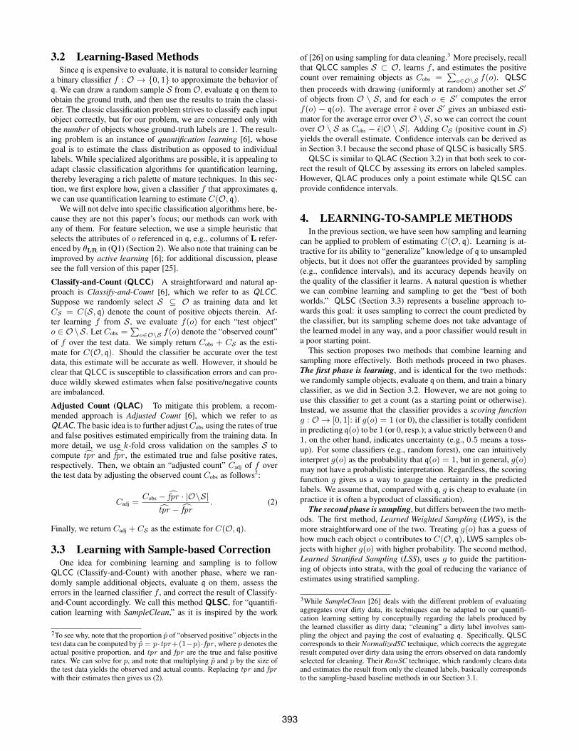
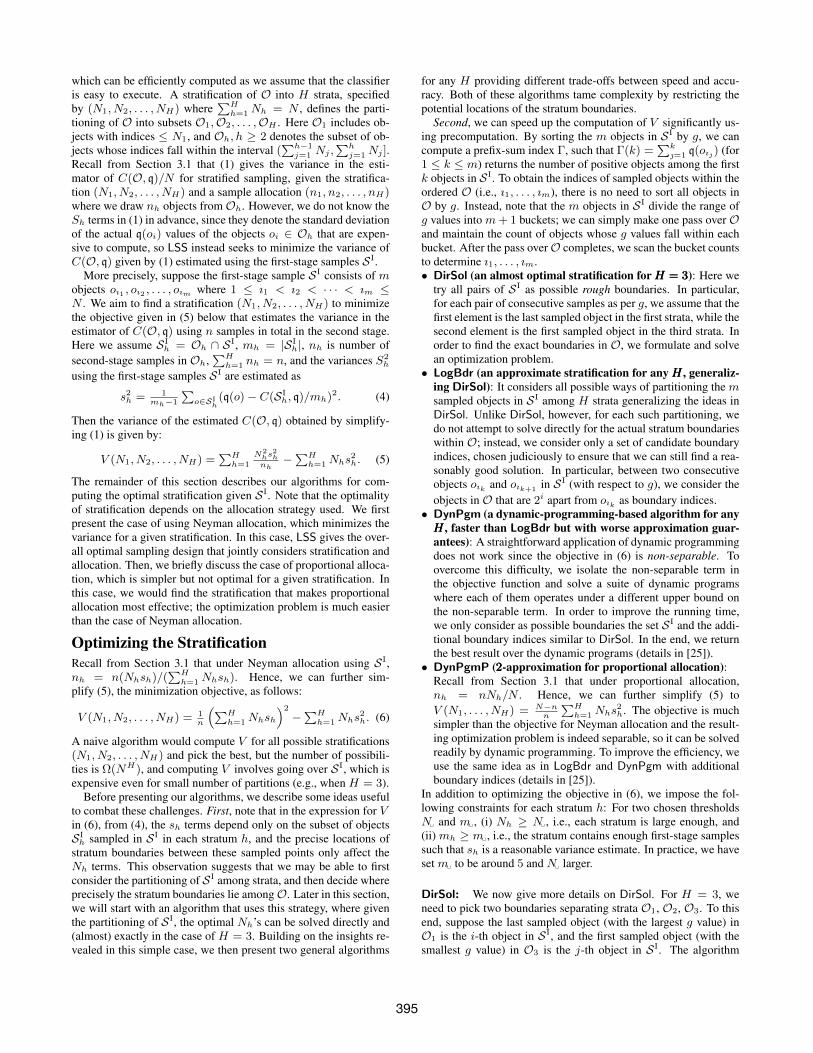
ing the three scenarios with real datasets, Neighbors, Sports. andText. Both LSS and LWS used a random forest classifier with esti-mators and a 25%:75% training:sampling split. Figure 1 comparesthe MAE of various algorithms when we vary the result size (viaquery parameters) while keeping the sample size fixed. Figure 2compares the MAE of various algorithms when we vary the samplesize while keeping the result size fixed.

As it turns out, the learned classifier performs pretty well forNeighbors and Sports, but pretty poorly for Text, leading to verydifferent results. We shall focus on Neighbors and Sports first. F1scores for the learned classifiers average higher than 0.8 in thesescenarios (with small result sizes being more difficult). We makeseveral observations. First, learning-based methods are very com-petitive here thanks to high classifier quality. In fact, QLCC some-times even delivers the smallest errors even without any adjustmentor correction. But to keep things in perspective, QLCC and QLACdo not provide any guarantees; once QLSC uses sampling to pro-vide correction and guarantees, MAE actually takes a small hit be-cause of the extra overhead. Second, algorithms without any learn-ing component, namely SRS and SSP are clearly not as competi-tive here, with much higher MAE than others. Third, LSS (high-lighted) has consistently low MAE; it is nearly always the leaderor not far from the leader, and bear in mind that it offers statisti-cal guarantees, which QLCC does not. LSS also consistently leadsQLSC by a good margin. Fourth, the comparison between LWSand LSS is difficult, as in some cases LWS leads LSS. The qualityof the learned classifier for Neighbors and Sports is the main factorhere. To better understand the situation, we take a closer look atsome data points with violin plots showing distributions.

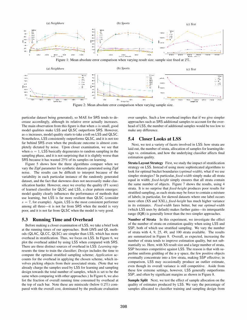
In Figure 3, we get a more detailed sense of the variability inestimates. LSS and LWS are consistently no worse and often betterthan SRS and SSP. Between LSS and LWS, we make two observa-tions. First, when selectivity is low, we expect all sampling-based

5A violin plot shows the probability density at different values; additionally,a white dot marks the median of all data, a thick black line spans the lowerand upper quartiles.

methods to have some trouble as the particular number of posi-tives that come up by chance in each run will have a large impacton relative error. For Sports, LWS dodged this issue with a verygood classifier that allows it to draw in a very targeted fashion.In contrast, LSS, as it places much less trust in the learned modelcompared with LWS, misses the opportunity. Second, LWS is notwithout its own problems. In Neighbors, where prediction becomesslightly more challenging, we see LWS underestimating with XSresult size; as it turns out, the classifier at those points happens togenerate more false negatives. In other words, LWS depends farmore on model quality than LSS does—it can benefit more, butalso can get hurt more. This effect will be magnified for the Textscenario, which we focus on next.

The Text tells a completely different story. In this case, classifica-tion is hard. Therefore, QLCC, QLAC, and QLSC fare very poorlyhere, because their performance is too dependent on starting pointproduced by QLCC. Correction is also difficult. From one repre-sentative run (with 857k resize size), true TPR and FPR are .53and .85, while the estimated TPR and FPR are .35 and .95. Evenwith sampling-based correction, QLSC still underperforms otheralgorithms. In contrast, SRS, which does not use learning, actuallyshines here. Finally, LSS tracks SRS closely. It actually underper-forms SRS a bit, which is understandable because learning phase isessentially not that useful, wasting 25% of the samples. However,the impact on the sampling design is limited. Closer examinationreveals that it basically degenerates to SRS for the remaining 75%of the samples. This experiment highlights the sensitivity of QLCC,QLAC, and QLSC toward poor models, as well as the resiliency ofLSS against poor models.

5.2 Comparison with Synthetic DatasetsResults in Section 5.1 show just three data points along the spec-

trum of classifier quality: Neighbors and Sports have good classi-fiers but Text has a bad one. What happens in between? To under-stand how different algorithms are affected by varying degrees ofdifficulty in using a learned model to approximate a predicate, wedesign our next set of experiments by injecting additional “noise”into the Sports scenario to adjust the difficulty of classification. Re-call from Example 2 that for each object o, we compute a countsubquery with o.x and o.y, and compare the resulting count, sayc, with k. Now, we create an additional “noise” table keyed ondistinct (x, y) values, where each (x, y) is associated with a noisecount drawn randomly from another distribution. Instead of com-paring cwith k, we use another subquery to look up the noise countc′ for (o.x, o.y), and have the predicate combine the original andnoise counts into (1− α)c+ αc′ to compare with k. By adjustingα ∈ [0, 1], we control how much noise contributes to the outcomeof the predicate: α = 0 corresponds to the original Sports scenario,where we know we can learn a good model; α = 1 means thepredicate is simply comparing independent random noise, which ismostly challenging to predict.

We experiment with two noise distributions. One is a Gaussianwith standard deviation of 1 truncated and discretized. The otheris derived from a Zipf distribution with parameter s, where eachdraw is used to index into a randomly permuted array of possiblenoise counts derived from the real count values; large smeans some(random) noise count will be far more popular than others.

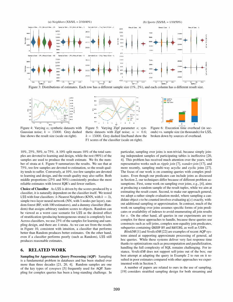
We compare SRS, QLSC, and LSS, representing sampling-based, learning-based (but with sampling-based correction), andlearn-to-sample algorithms, respectively. Figure 4 shows how theycompare in terms of MAE when we vary α for synthetic datasetsgenerated using Gaussian noise. Note that when α increases, theresult size tends to decrease (but it is random depending on the

397

(a) Neighbors (b) Sports (c) Text

Figure 1: Mean absolute error comparison when varying result size; sample size fixed at 2%.

(a) Neighbors (b) Sports (c) Text

Figure 2: Mean absolute error comparison when varying sample size.

particular dataset being generated), so MAE for SRS tends to de-crease accordingly, although its relative error actually increases.The main observation from this figure is that when α is small, goodmodel qualities make LSS and QLSC outperform SRS. However,as α increases, model quality starts to take a toll on LSS and QLSC.Nonetheless, LSS consistently outperforms QLSC, and it is not toofar behind SRS even when the predicate outcome is almost com-pletely dictated by noise. Upon closer examination, we see thatwhen α = 1, LSS basically degenerates to random sampling in thesampling phase, and it is not surprising that it is slightly worse thanSRS because it has wasted 25% of its samples on learning.

Figure 5 shows how the three algorithms compare when wevary the Zipf parameter for synthetic datasets generated using Zipfnoise. The results can be difficult to interpret because of thevariability in each particular instance of the randomly generateddataset, and the fact that skewness does not necessarily make clas-sification harder. However, once we overlay the quality (F1 score)of learned classifier for QLSC and LSS, a clear pattern emerges:model quality clearly influences the performance of methods thatuse learning, but LSS is far more resilient than QLSC (considers = 7, for example). Again, LSS is the most consistent performeramong all three—it is not far from SRS when the model is verypoor, and it is not far from QLSC when the model is very good.

5.3 Running Time and OverheadBefore making a closer examination of LSS, we take a brief look

at the running times of our approaches. Both LWS and QL meth-ods (QLAC, QLCC, QLSC) are simpler than LSS, which has moreoverhead in stratification. Thus, we focus on LSS. In Figure 6, weplot the overhead added by using LSS when compared with SRS.There are three distinct sources of overhead in LSS: Learning rep-resents the time to train the classifier; Design includes the time tocompute the optimal stratified sampling scheme; Application ac-counts for the overhead in applying the chosen scheme, which in-volves picking objects from their associated strata. (Note that wealready charge the samples used by LSS for learning and samplingdesign towards the total number of samples, which is set to be thesame when comparing with other approaches.) In Figure 6, we alsolist the fraction of overall running time consumed by overhead atthe top of each bar. Note these are miniscule (below 0.2%) com-pared with the overall cost, dominated by the predicate evaluation

over samples. Such a low overhead implies that if we give simplerapproaches such as SRS additional samples to account for the over-head of LSS, the number of additional samples would be too low tomake any difference.

5.4 Closer Looks at LSSNext, we test a variety of facets involved in LSS: how strata are

laid out, the number of strata, allocation of samples for learning/de-sign vs. estimation, and how the underlying classifier affects finalestimation quality.

Strata Layout Strategy First, we study the impact of stratificationstrategy on LSS. Instead of using more sophisticated algorithms tolook for optimal bucket boundaries (optimal-width), what if we usesimpler strategies? In particular, fixed-width simply make all strataequal in width; fixed-height simply ensures that all strata containthe same number of objects. Figure 7 shows the results, using 4strata. It is no surprise that fixed-height produces poor results forstratified sampling, as each strata may be force to contain a mixtureof labels; in particular, for skewed datasets where one label occursmore often (XS and XXL), fixed-height has much higher variancein its estimates. Fixed-width fares better, but our optimal-width(which LSS uses by default) makes further gains—its interquartilerange (IQR) is generally lower than the two simpler approaches.

Number of Strata In this experiment, we investigate the effectof the number of strata on estimation quality when using LSS andSSP, both of which use stratified sampling. We vary the numberof strata with 4, 9, 25, 49, and 100 strata available. The resultsare summarized in Figure 8. Overall, as expected, increasing thenumber of strata tends to improve estimation quality, but not sub-stantially so. Here, with XS result size and a large number of strata,SSP becomes competitive against LSS. The reason is that with su-perfine uniform gridding of the x-y space, the few positive objectseventually concentrate into a few strata, making SSP effective; incomparison, LSS may occasionally produce an outlier estimate,even though its overall variance is still competitive. Aside fromthese few extreme settings, however, LSS generally outperformsSSP, and often by significant margins as shown in Figure 8.

Sample Split Next, we test the effect of sample allocation on thequality of estimates produced by LSS. We vary the percentage ofsamples allocated to classifier training and sampling design from

398

(a) Neighbors (XS/S/L = 2/10/40%) (b) Sports (XS/S/L = 1/10/50%)

Figure 3: Distributions of estimates. Each row has a different sample size (1%, 2%), and each column has a different result size.

Figure 4: Varying α; synthetic datasets withGaussian noise; k = 15000. Grey dashedline shows the result size (scale on right).

Figure 5: Varying Zipf parameter s; syn-thetic datasets with Zipf noise; α = 0.6;k = 15000. Grey dashed line/band show theF1 scores of the classifier (scale on right).

Figure 6: Execution time overhead (in sec-onds) vs. sample size (in thousands) for LSS,broken down by sources of overhead.

10%, 25%, 50%, to 75%. A 10% split means 10% of the total sam-ples are devoted to learning and design, while the rest (90%) of thesamples are used to produce the result estimate. We fix the num-ber of strata at 4. Figure 9 summarizes the results. We see that at75%, too few samples are devoted to estimation, so the result qual-ity tends to suffer. Conversely, at 10%, too few samples are devotedto learning and design, and the result quality may also suffer. Bothmiddle proportions (25% and 50%) consistently produce the mostreliable estimates with lowest IQR’s and fewer outliers.

Choice of Classifier As LSS is driven by the scores produced by aclassifier, it is naturally dependent on the classifier itself. We testedLSS with four classifiers: k-Nearest Neighbors (KNN, with k = 3),simple two-layer neural network (NN, with 5 nodes per layer), ran-dom forest (RF, with 100 estimators), and a dummy classifier (Ran-dom) that assigns arbitrary random scores to objects. Random canbe viewed as a worst case scenario for LSS as the desired effectof stratification (producing homogeneous strata) is completely lost.Across classifiers, we use 25% of the samples for learning and sam-pling design, and there are 4 strata. As we can see from the resultsin Figure 10, consistent with intuition, a classifier that performsbetter than Random produces better estimates. On the other hand,even if a classifier performs poorly (such as Random), LSS stillproduces reasonable estimates.

6. RELATED WORKSampling for Approximate Query Processing (AQP) Samplingis a fundamental problem in databases and has been studied overmore than three decades [21, 20, 4]. Random samples are oneof the key types of synopses [5] frequently used for AQP. Sam-pling for complex queries has been a long-standing challenge. In

particular, sampling over joins is non-trivial, because simply join-ing independent samples of participating tables is ineffective [20,4]. This problem has received much attention over the years, withrepresentative works such as ripple join [7], wander-join [17], andmore recently, sampling multi-way acyclic and cyclic joins [27].The focus of our work is on counting queries with complex pred-icates. Even though our predicates can include joins as discussedin Section 2, our techniques differ because of different problem as-sumptions. First, some work on sampling over joins, e.g., [4], aimsat producing a random sample of the result tuples, while we aim atestimating the result count. Second, to make our approach general,we adopt a rather simple evaluation model, where sampling a can-didate object o to be counted involves evaluating q(o) exactly, with-out additional sampling or approximation. In contrast, much of thework on sampling over joins assumes specific forms of join predi-cates or availability of indexes to avoid enumerating all join resultsfor o. On the other hand, all queries in our experiments are toocomplex for these approaches to handle, because these queries useconstructs such as self-joins, complex non-equality join predicates,subqueries containing GROUP BY and HAVING, as well as UDFs.

BlinkDB [1] and VerdictDB [22] are examples of recent AQP sys-tems aimed at supporting approximate processing of general, adhoc queries. While these systems deliver very fast response timethanks to optimizations such as precomputation and parallelization,handling the full complexity of SQL remains challenging. For in-stance, VerdictDB does not support self-joins out of the box; ourbest attempt at adapting the query in Example 2 to run on it re-sulted in poor estimates compared with other approaches we exper-imented with in Section 5.

A number of papers are related to ours in the use of sampling.[19] considers stratified sampling design for both streaming and

399

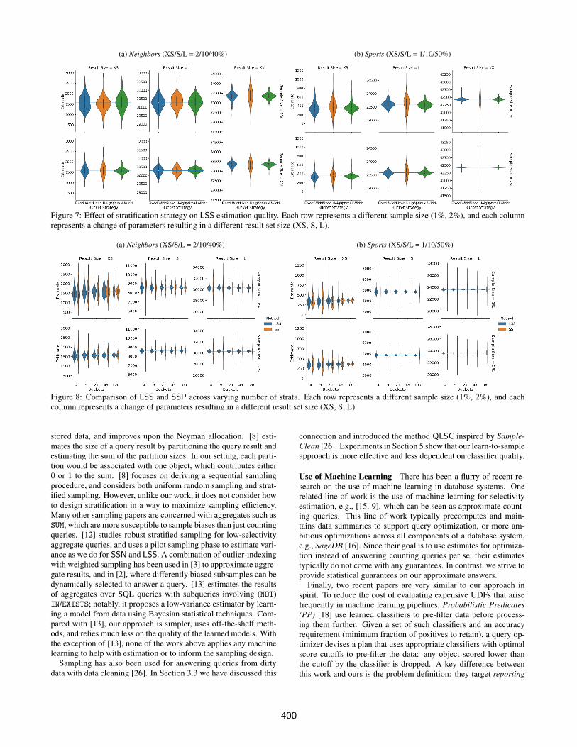
(a) Neighbors (XS/S/L = 2/10/40%) (b) Sports (XS/S/L = 1/10/50%)

Figure 7: Effect of stratification strategy on LSS estimation quality. Each row represents a different sample size (1%, 2%), and each columnrepresents a change of parameters resulting in a different result set size (XS, S, L).

(a) Neighbors (XS/S/L = 2/10/40%) (b) Sports (XS/S/L = 1/10/50%)

Figure 8: Comparison of LSS and SSP across varying number of strata. Each row represents a different sample size (1%, 2%), and eachcolumn represents a change of parameters resulting in a different result set size (XS, S, L).

stored data, and improves upon the Neyman allocation. [8] esti-mates the size of a query result by partitioning the query result andestimating the sum of the partition sizes. In our setting, each parti-tion would be associated with one object, which contributes either0 or 1 to the sum. [8] focuses on deriving a sequential samplingprocedure, and considers both uniform random sampling and strat-ified sampling. However, unlike our work, it does not consider howto design stratification in a way to maximize sampling efficiency.Many other sampling papers are concerned with aggregates such asSUM, which are more susceptible to sample biases than just countingqueries. [12] studies robust stratified sampling for low-selectivityaggregate queries, and uses a pilot sampling phase to estimate vari-ance as we do for SSN and LSS. A combination of outlier-indexingwith weighted sampling has been used in [3] to approximate aggre-gate results, and in [2], where differently biased subsamples can bedynamically selected to answer a query. [13] estimates the resultsof aggregates over SQL queries with subqueries involving (NOT)IN/EXISTS; notably, it proposes a low-variance estimator by learn-ing a model from data using Bayesian statistical techniques. Com-pared with [13], our approach is simpler, uses off-the-shelf meth-ods, and relies much less on the quality of the learned models. Withthe exception of [13], none of the work above applies any machinelearning to help with estimation or to inform the sampling design.

Sampling has also been used for answering queries from dirtydata with data cleaning [26]. In Section 3.3 we have discussed this

connection and introduced the method QLSC inspired by Sample-Clean [26]. Experiments in Section 5 show that our learn-to-sampleapproach is more effective and less dependent on classifier quality.

Use of Machine Learning There has been a flurry of recent re-search on the use of machine learning in database systems. Onerelated line of work is the use of machine learning for selectivityestimation, e.g., [15, 9], which can be seen as approximate count-ing queries. This line of work typically precomputes and main-tains data summaries to support query optimization, or more am-bitious optimizations across all components of a database system,e.g., SageDB [16]. Since their goal is to use estimates for optimiza-tion instead of answering counting queries per se, their estimatestypically do not come with any guarantees. In contrast, we strive toprovide statistical guarantees on our approximate answers.

Finally, two recent papers are very similar to our approach inspirit. To reduce the cost of evaluating expensive UDFs that arisefrequently in machine learning pipelines, Probabilistic Predicates(PP) [18] use learned classifiers to pre-filter data before process-ing them further. Given a set of such classifiers and an accuracyrequirement (minimum fraction of positives to retain), a query op-timizer devises a plan that uses appropriate classifiers with optimalscore cutoffs to pre-filter the data: any object scored lower thanthe cutoff by the classifier is dropped. A key difference betweenthis work and ours is the problem definition: they target reporting

400

(a) Neighbors (XS/S/L = 2/10/40%) (b) Sports (XS/S/L = 1/10/50%)

Figure 9: LSS as the percentage of samples used for learning/design (instead of producing the result estimate) varies. Each row represents adifferent sample size (1%, 2%), and each column represents a change of parameters resulting in a different result set size (XS, S, L).

(a) Neighbors (XS/S/L = 2/10/40%) (b) Sports (XS/S/L = 1/10/50%)

Figure 10: LSS under different classifiers. Each row represents a different sample size (1%, 2%), and each column represents a change ofparameters resulting in a different result set size (XS, S, L).

queries while we target counting queries. This difference leads toour different use of the classifier scores; applying PP to our settingwould result in poor estimates. Furthermore, PP gives no statisti-cal guarantees on the actual recall, and its performance is far moresusceptible to bad classifiers because of its heavy reliance on clas-sifier scores. Earlier work by Joglekar et al. [11] similarly tacklesqueries involving selections with expensive UDFs. By identifyingattributes whose values are correlated with UDF results, and group-ing objects by the values of such attributes, they judiciously choosethe appropriate actions to take for each group of objects (e.g., ac-cept all, return all, or sample some). Like our approach, the use ofsampling enables probabilistic guarantees, but the key differenceremains that they target reporting instead of counting queries.

7. CONCLUSION AND FUTURE WORKIn this paper, we have developed new techniques to estimate the

results of counting queries with complex filters. Our techniquesare based on a simple yet powerful idea: replace an expensive fil-ter with a cheap classifier that approximates the filter. This cheapclassifier can then be used in a number of different ways with dif-ferent trade-offs. A key challenge is that too much reliance on theclassifier makes result quality highly susceptible to bad classifiers.However, one novel technique we proposed, learned stratified sam-pling, delivers consistently good estimates compared with other al-

ternatives. It is very resilient against bad classifiers, thanks to howit combines machine learning and sampling—the learned classifieris used in a limited but helpful way to design a stratified samplingscheme which in turn produces the estimate. This resiliency makesthe technique easy to apply in practice, because we are much lessconcerned with training a perfect model: a good model will makesampling more efficient, but even if the model is poor and/or thefilter is fundamentally hard to approximate, the technique still de-livers unbiased estimates with statistical guarantees comparable torandom sampling. There is an abundance of future work. In partic-ular, learned stratified sampling is quite conservative by design—toensure independence, it avoids using the samples it acquired in thelearning phase when computing the final estimate. However, theremay be ways in which such samples can be safely used. Second,some of the queries we considered in this paper (such as skybandsizes and neighbor counts) have highly specialized solutions. Al-though our goal is to develop general solutions that can work forfar more complex queries, it will still be interesting to carry out adirect comparison with the specialized solutions for these specificqueries. Finally, a promising direction is to extend and fully evalu-ate our approach in an online aggregation [10] setting.

401

8. REFERENCES[1] S. Agarwal, B. Mozafari, A. Panda, H. Milner, S. Madden,

and I. Stoica. Blinkdb: Queries with bounded errors andbounded response times on very large data. In Proceedings ofthe 8th ACM European Conference on Computer Systems,EuroSys ’13, pages 29–42, New York, NY, USA, 2013.ACM.

[2] B. Babcock, S. Chaudhuri, and G. Das. Dynamic sampleselection for approximate query processing. In Proceedingsof the 2003 ACM SIGMOD International Conference onManagement of Data, SIGMOD ’03, pages 539–550, NewYork, NY, USA, 2003. ACM.

[3] S. Chaudhuri, G. Das, M. Datar, R. Motwani, and V. R.Narasayya. Overcoming limitations of sampling foraggregation queries. In Proceedings of the 17th InternationalConference on Data Engineering, April 2-6, 2001,Heidelberg, Germany, pages 534–542, 2001.

[4] S. Chaudhuri, R. Motwani, and V. Narasayya. On RandomSampling over Joins. In Proceedings of the 1999 ACMSIGMOD International Conference on Management of Data,SIGMOD ’99, pages 263–274, New York, NY, USA, 1999.ACM.

[5] G. Cormode, M. Garofalakis, P. J. Haas, and C. Jermaine.Synopses for massive data: Samples, histograms, wavelets,sketches. Foundations and Trends R© in Databases,4(1–3):1–294, 2011.

[6] P. Gonzlez, A. Castao, N. V. Chawla, and J. J. D. Coz. AReview on Quantification Learning. ACM Comput. Surv.,50(5):74:1–74:40, Sept. 2017.

[7] P. J. Haas and J. M. Hellerstein. Ripple Joins for OnlineAggregation. In Proceedings of the 1999 ACM SIGMODInternational Conference on Management of Data, SIGMOD’99, pages 287–298, New York, NY, USA, 1999. ACM.

[8] P. J. Haas and A. N. Swami. Sequential sampling proceduresfor query size estimation. In Proceedings of the 1992 ACMSIGMOD International Conference on Management of Data,SIGMOD ’92, pages 341–350, New York, NY, USA, 1992.ACM.

[9] M. Halford, P. Saint-Pierre, and F. Morvan. An approachbased on bayesian networks for query selectivity estimation.In DASFAA (2), volume 11447 of Lecture Notes in ComputerScience, pages 3–19. Springer, 2019.

[10] J. M. Hellerstein, P. J. Haas, and H. J. Wang. Onlineaggregation. In Proceedings of the 1997 ACM SIGMODInternational Conference on Management of Data, SIGMOD’97, pages 171–182, New York, NY, USA, 1997. ACM.

[11] M. Joglekar, H. Garcia-Molina, A. Parameswaran, andC. Re. Exploiting Correlations for Expensive PredicateEvaluation. In Proceedings of the 2015 ACM SIGMODInternational Conference on Management of Data, SIGMOD’15, pages 1183–1198, New York, NY, USA, 2015. ACM.

[12] S. Joshi and C. M. Jermaine. Robust stratified sampling plansfor low selectivity queries. In Proceedings of the 24thInternational Conference on Data Engineering, ICDE 2008,April 7-12, 2008, Cancun, Mexico, pages 199–208, 2008.

[13] S. Joshi and C. M. Jermaine. Sampling-based estimators forsubset-based queries. PVLDB, 18(1):181–202, 2009.

[14] G. Kalton, K. Graham, et al. Introduction to survey sampling,volume 35. Sage, 1983.

[15] A. Kipf, T. Kipf, B. Radke, V. Leis, P. A. Boncz, andA. Kemper. Learned cardinalities: Estimating correlatedjoins with deep learning. In CIDR 2019, 9th BiennialConference on Innovative Data Systems Research, Asilomar,CA, USA, January 13-16, 2019, Online Proceedings, 2019.

[16] T. Kraska, M. Alizadeh, A. Beutel, E. H. Chi, A. Kristo,G. Leclerc, S. Madden, H. Mao, and V. Nathan. Sagedb: Alearned database system. In CIDR 2019, 9th BiennialConference on Innovative Data Systems Research, Asilomar,CA, USA, January 13-16, 2019, Online Proceedings, 2019.

[17] F. Li, B. Wu, K. Yi, and Z. Zhao. Wander Join: OnlineAggregation via Random Walks. In Proceedings of the 2016International Conference on Management of Data, SIGMOD’16, pages 615–629, New York, NY, USA, 2016. ACM.

[18] Y. Lu, A. Chowdhery, S. Kandula, and S. Chaudhuri.Accelerating Machine Learning Inference with ProbabilisticPredicates. In Proceedings of the 2018 InternationalConference on Management of Data, SIGMOD ’18, pages1493–1508, New York, NY, USA, 2018. ACM.

[19] T. D. Nguyen, M. Shih, D. Srivastava, S. Tirthapura, andB. Xu. Stratified random sampling over streaming and storeddata. In Advances in Database Technology - 22ndInternational Conference on Extending DatabaseTechnology, EDBT 2019, Lisbon, Portugal, March 26-29,2019, pages 25–36, 2019.

[20] F. Olken and F. Olken. Random sampling from databases.Ph.D. thesis, U.C. Berkeley, 1993.

[21] F. Olken and D. Rotem. Simple Random Sampling fromRelational Databases. In Proceedings of the 12thInternational Conference on Very Large Data Bases, VLDB,pages 160–169, San Francisco, CA, USA, 1986. MorganKaufmann Publishers Inc.

[22] Y. Park, B. Mozafari, J. Sorenson, and J. Wang. Verdictdb:Universalizing approximate query processing. InProceedings of the 2018 International Conference onManagement of Data, SIGMOD Conference 2018, Houston,TX, USA, June 10-15, 2018, pages 1461–1476, 2018.

[23] I. Partalas, A. Kosmopoulos, N. Baskiotis, T. Artieres,G. Paliouras, E. Gaussier, I. Androutsopoulos, M.-R. Amini,and P. Galinari. Lshtc: A benchmark for large-scale textclassification, 2015.

[24] Y. Tille. Sampling algorithms. In International Encyclopediaof Statistical Science, pages 1273–1274. Springer, 2011.

[25] B. Walenz, S. Sintos, S. Roy, and J. Yang. Learning tosample: Counting with complex queries.https://arxiv.org/abs/1906.09335.

[26] J. Wang, S. Krishnan, M. J. Franklin, K. Goldberg, T. Kraska,and T. Milo. A sample-and-clean framework for fast andaccurate query processing on dirty data. In InternationalConference on Management of Data, SIGMOD 2014,Snowbird, UT, USA, June 22-27, 2014, pages 469–480, 2014.

[27] Z. Zhao, R. Christensen, F. Li, X. Hu, and K. Yi. Randomsampling over joins revisited. In Proceedings of the 2018International Conference on Management of Data, SIGMOD’18, pages 1525–1539, New York, NY, USA, 2018. ACM.

402