Learning to Map between Ontologies.pdf

7/26/2019 Learning to Map between Ontologies.pdf

http://slidepdf.com/reader/full/learning-to-map-between-ontologiespdf 1/12

Learning to Map between Ontologieson the Semantic Web

AnHai Doan, Jayant Madhavan, Pedro Domingos, and Alon HalevyComputer Science and Engineering

University of Washington, Seattle, WA, USA

{anhai, jayant, pedrod, alon}@cs.washington.edu

ABSTRACT

Ontologies play a prominent role on the Semantic Web.They make possible the widespread publication of machineunderstandable data, opening myriad opportunities for au-tomated information processing. However, because of theSemantic Web’s distributed nature, data on it will inevitablycome from many different ontologies. Information process-ing across ontologies is not possible without knowing the

semantic mappings between their elements. Manually find-ing such mappings is tedious, error-prone, and clearly notpossible at the Web scale. Hence, the development of toolsto assist in the ontology mapping process is crucial to thesuccess of the Semantic Web.

We describe GLUE, a system that employs machine learn-ing techniques to find such mappings. Given two ontologies,for each concept in one ontology GLUE finds the most sim-ilar concept in the other ontology. We give well-foundedprobabilistic definitions to several practical similarity mea-sures, and show that GLUE can work with all of them. Thisis in contrast to most existing approaches, which deal witha single similarity measure. Another key feature of GLUEis that it uses multiple learning strategies, each of whichexploits a different type of information either in the data

instances or in the taxonomic structure of the ontologies.To further improve matching accuracy, we extend GLUEto incorporate commonsense knowledge and domain con-straints into the matching process. For this purpose, weshow that relaxation labeling , a well-known constraint opti-mization technique used in computer vision and other fields,can be adapted to work efficiently in our context. Our ap-proach is thus distinguished in that it works with a varietyof well-defined similarity notions and that it efficiently in-corporates multiple types of knowledge. We describe a set of experiments on several real-world domains, and show thatGLUE proposes highly accurate semantic mappings.

Categories and Subject Descriptors

I.2.6 [Computing Methodologies]: Artificial Intelligence—Learning ; H.2.5 [Information Systems]: Database Man-agement—Heterogenous Databases, Data translation

General Terms

Algorithms, Design, Experimentation.

Copyright is held by the author/owner(s).WWW2002 , May 7–11, 2002, Honolulu, Hawaii, USA.ACM 1-58113-449-5/02/0005.

Keywords

Semantic Web, Ontology Mapping, Machine Learning, Re-laxation Labeling.

1. INTRODUCTIONThe current World-Wide Web has well over 1.5 billion

pages [3], but the vast majority of them are in human-readable format only (e.g., HTML). As a consequence soft-

ware agents (softbots) cannot understand and process thisinformation, and much of the potential of the Web has sofar remained untapped.

In response, researchers have created the vision of theSemantic Web [6], where data has structure and ontolo-gies describe the semantics of the data. Ontologies allowusers to organize information into taxonomies of concepts,each with their attributes, and describe relationships be-tween concepts. When data is marked up using ontologies,softbots can better understand the semantics and thereforemore intelligently locate and integrate data for a wide vari-ety of tasks. The following example illustrates the vision of the Semantic Web.

Example 1.1. Suppose you want to find out more aboutsomeone you met at a conference. You know that his lastname is Cook, and that he teaches Computer Science at anearby university, but you do not know which one. You alsoknow that he just moved to the US from Australia, wherehe had been an associate professor at his alma mater.

On the World-Wide Web of today you will have troublefinding this person. The above information is not containedwithin a single Web page, thus making keyword search inef-fective. On the Semantic Web, however, you should be ableto quickly find the answers. A marked-up directory servicemakes it easy for your personal softbot to find nearby Com-puter Science departments. These departments have markedup data using some ontology such as the one in Figure 1.a.Here the data is organized into a taxonomy that includes

courses, people, and professors. Professors have attributes such as name, degree, and degree-granting institution. Suchmarked-up data makes it easy for your softbot to find a pro-fessor with the last name Cook. Then by examining the at-tribute “granting institution”, the softbot quickly finds thealma mater CS department in Australia. Here, the softbotlearns that the data has been marked up using an ontol-ogy specific to Australian universities, such as the one inFigure 1.b, and that there are many entities named Cook.However, knowing that “associate professor” is equivalent to“senior lecturer”, the bot can select the right subtree in the



departmental taxonomy, and zoom in on the old homepageof your conference acquaintance.

The Semantic Web thus offers a compelling vision, but italso raises many difficult challenges. Researchers have beenactively working on these challenges, focusing on fleshing outthe basic architecture, developing expressive and efficientontology languages, building techniques for efficient markingup of data, and learning ontologies (e.g., [15, 8, 30, 23, 4]).

A key challenge in building the Semantic Web, one thathas received relatively little attention, is finding semantic mappings among the ontologies . Given the de-centralizednature of the development of the Semantic Web, there willbe an explosion in the number of ontologies. Many of theseontologies will describe similar domains, but using differentterminologies, and others will have overlapping domains. Tointegrate data from disparate ontologies, we must know thesemantic correspondences between their elements [6, 35].For example, in the conference-acquaintance scenario de-scribed earlier, in order to find the right person, your softbotmust know that “associate professor” in the US correspondsto “senior lecturer” in Australia. Thus, the semantic corre-spondences are in effect the “glue” that hold the ontologiestogether into a “web of semantics”. Without them, the Se-

mantic Web is akin to an electronic version of the Tower of Babel. Unfortunately, manually specifying such correspon-dences is time-consuming, error-prone [28], and clearly notpossible on the Web scale. Hence, the development of toolsto assist in ontology mapping is crucial to the success of theSemantic Web [35].

In this paper we describe the GLUE system, which ap-plies machine learning techniques to semi-automatically cre-ate such semantic mappings. Since taxonomies are centralcomponents of ontologies, we focus first on finding corre-spondences among the taxonomies of two given ontologies:for each concept node in one taxonomy, find the most similar concept node in the other taxonomy.

The first issue we address in this realm is: what is themeaning of similarity between two concepts? Clearly, manydifferent definitions of similarity are possible, each being ap-propriate for certain situations. Our approach is based onthe observation that many practical measures of similaritycan be defined based solely on the joint probability distribu-tion of the concepts involved. Hence, instead of committingto a particular definition of similarity, GLUE calculates the joint distribution of the concepts, and lets the applicationuse the joint distribution to compute any suitable similaritymeasure. Specifically, for any two concepts A and B, wecompute P (A, B), P (A, B), P (A, B), and P (A, B), where aterm such as P (A, B) is the probability that an instance inthe domain belongs to concept A but not to concept B . Anapplication can then define similarity to be a suitable func-tion of these four values. For example, a similarity measure

we use in this paper is P (A∩B)/P (A∪B), otherwise knownas the Jaccard coefficient [36].

The second challenge we address is that of computing the joint distribution of any two given concepts A and B. Undercertain general assumptions (discussed in Section 4), a termsuch as P (A, B) can be approximated as the fraction of in-stances that belong to both A and B (in the data associatedwith the taxonomies or, more generally, in the probabilitydistribution that generated it). Hence, the problem reducesto deciding for each instance if it belongs to A ∩ B. How-ever, the input to our problem includes instances of A and

instances of B in isolation. GLUE addresses this problemusing machine learning techniques as follows: it uses the in-stances of A to learn a classifier for A, and then classifiesinstances of B according to that classifier, and vice-versa.Hence, we have a method for identifying instances of A ∩B.

Applying machine learning to our context raises the ques-tion of which learning algorithm to use and which typesof information to use in the learning process. Many differ-ent types of information can contribute toward deciding the

membership of an instance: its name, value format, the wordfrequencies in its value, and each of these is best utilized bya different learning algorithm. GLUE uses a multi-strategy learning approach [12]: we employ a set of learners, thencombine their predictions using a meta-learner. In previouswork [12] we have shown that multi-strategy learning is ef-fective in the context of mapping between database schemas.

Finally, GLUE attempts to exploit available domain con-straints and general heuristics in order to improve matchingaccuracy. An example heuristic is the observation that twonodes are likely to match if nodes in their neighborhoodalso match. An example of a domain constraint is “if nodeX matches Professor and node Y is an ancestor of X inthe taxonomy, then it is unlikely that Y matches Assistant-

Professor”. Such constraints occur frequently in practice,and heuristics are commonly used when manually mappingbetween ontologies. Previous works have exploited only oneform or the other of such knowledge and constraints, in re-strictive settings [29, 26, 21, 25]. Here, we develop a unifyingapproach to incorporate all such types of information. Ourapproach is based on relaxation labeling , a powerful tech-nique used extensively in the vision and image processingcommunity [16], and successfully adapted to solve matchingand classification problems in natural language processing[31] and hypertext classification [10]. We show that relax-ation labeling can be adapted efficiently to our context, andthat it can successfully handle a broad variety of heuristicsand domain constraints.

In the rest of the paper we describe the GLUE system and

the experiments we conducted to validate it. Specifically,the paper makes the following contributions:

• We describe well-founded notions of semantic similar-ity, based on the joint probability distribution of theconcepts involved. Such notions make our approachapplicable to a broad range of ontology-matching prob-lems that employ different similarity measures.

• We describe the use of multi-strategy learning for find-ing the joint distribution, and thus the similarity valueof any concept pair in two given taxonomies. TheGLUE system, embodying our approach, utilizes manydifferent types of information to maximize matchingaccuracy. Multi-strategy learning also makes our sys-

tem easily extensible to additional learners, as theybecome available.

• We introduce relaxation labeling to the ontology-match-ing context, and show that it can be adapted to effi-ciently exploit a broad range of common knowledgeand domain constraints to further improve matchingaccuracy.

• We describe a set of experiments on several real-worlddomains to validate the effectiveness of GLUE. Theresults show the utility of multi-strategy learning and



CS Dept US CS Dept Australia

UnderGrad

Courses

Grad

CoursesCourses StaffPeople

StaffFaculty

AssistantProfessor

AssociateProfessor

Professor

Technical StaffAcademic Staff

Lecturer SeniorLecturer

Professor

- name

- degree

- granting - institution

- first -name

- last -name

- education

R.Cook

Ph.D.

Univ. of Sydney

K. Burn

Ph.D.

Univ. of Michigan

(a) (b)

Figure 1: Computer Science Department Ontologies

relaxation labeling, and that GLUE can work well withdifferent notions of similarity.

In the next section we define the ontology-matching prob-lem. Section 3 discusses our approach to measuring similar-ity, and Sections 4-5 describe the GLUE system. Section 6presents our experiments. Section 7 reviews related work.Section 8 discusses future work and concludes.

2. ONTOLOGY MATCHINGWe now introduce ontologies, then define the problem of

ontology matching. An ontology specifies a conceptualiza-tion of a domain in terms of concepts, attributes, and rela-tions [14]. The concepts provided model entities of interestin the domain. They are typically organized into a taxon-omy tree where each node represents a concept and eachconcept is a specialization of its parent. Figure 1 shows twosample taxonomies for the CS department domain (whichare simplifications of real ones).

Each concept in a taxonomy is associated with a set of instances . For example, concept Associate-Professor has in-stances “Prof. Cook” and “Prof. Burn” as shown in Fig-ure 1.a. By the taxonomy’s definition, the instances of aconcept are also instances of an ancestor concept. For ex-ample, instances of Assistant-Professor, Associate-Professor,and Professor in Figure 1.a are also instances of Faculty andPeople.

Each concept is also associated with a set of attributes .For example, the concept Associate-Professor in Figure 1.ahas the attributes name, degree, and granting-institution. Aninstance that belongs to a concept has fixed attribute values.

For example, the instance “Professor Cook” has value name= “R. Cook”, degree = “Ph.D.”, and so on. An ontology alsodefines a set of relations among its concepts. For example, arelation AdvisedBy(Student,Professor) might list all instancepairs of Student and Professor such that the former is advisedby the latter.

Many formal languages to specify ontologies have beenproposed for the Semantic Web, such as OIL, DAML+OIL,SHOE, and RDF [8, 2, 15, 7]. Though these languages differin their terminologies and expressiveness, the ontologies thatthey model essentially share the same features we described

above.Given two ontologies, the ontology-matching problem is to

find semantic mappings between them. The simplest typeof mapping is a one-to-one (1-1) mapping between the ele-ments, such as “Associate-Professor maps to Senior-Lecturer”,and “degree maps to education”. Notice that mappings be-tween different types of elements are possible, such as “therelation AdvisedBy(Student,Professor) maps to the attributeadvisor of the concept Student”. Examples of more complextypes of mapping include “name maps to the concatenationof first-name and last-name”, and “the union of Undergrad-Courses and Grad-Courses maps to Courses”. In general, amapping may be specified as a query that transforms in-stances in one ontology into instances in the other [9].

In this paper we focus on finding 1-1 mappings betweenthe taxonomies. This is because taxonomies are central com-ponents of ontologies, and successfully matching them would

greatly aid in matching the rest of the ontologies. Extendingmatching to attributes and relations and considering morecomplex types of matching is the subject of ongoing research.

There are many ways to formulate a matching problemfor taxonomies. The specific problem that we consider isas follows: given two taxonomies and their associated data instances, for each node (i.e., concept) in one taxonomy, find the most similar node in the other taxonomy, for a pre-defined similarity measure . This is a very general problemsetting that makes our approach applicable to a broad rangeof common ontology-related problems on the Semantic Web,such as ontology integration and data translation among theontologies.

Data instances: GLUE makes heavy use of the fact that

we have data instances associated with the ontologies we arematching. We note that many real-world ontologies alreadyhave associated data instances. Furthermore, on the Se-mantic Web, the largest benefits of ontology matching comefrom matching the most heavily used ontologies; and themore heavily an ontology is used for marking up data, themore data it has. Finally, we show in our experiments thatonly a moderate number of data instances is necessary inorder to obtain good matching accuracy.



3. SIMILARITY MEASURESTo match concepts between two taxonomies, we need a

notion of similarity. We now describe the similarity mea-sures that GLUE handles; but before doing that, we discussthe motivations leading to our choices.

First, we would like the similarity measures to be well-defined. A well-defined measure will facilitate the evaluationof our system. It also makes clear to the users what the sys-tem means by a match, and helps them figure out whetherthe system is applicable to a given matching scenario. Fur-thermore, a well-defined similarity notion may allow us toleverage special-purpose techniques for the matching pro-cess.

Second, we want the similarity measures to correspondto our intuitive notions of similarity. In particular, theyshould depend only on the semantic content of the conceptsinvolved, and not on their syntactic specification.

Finally, it is clear that many reasonable similarity mea-sures exist, each being appropriate to certain situations.Hence, to maximize our system’s applicability, we wouldlike it to be able to handle a broad variety of similaritymeasures. The following examples illustrate the variety of possible definitions of similarity.

Example 3.1. In searching for your conference acquain-tance, your softbot should use an “exact” similarity measurethat maps Associate-Professor into Senior Lecturer, an equiv-alent concept. However, if the softbot has some postprocess-ing capabilities that allow it to filter data, then it may tol-erate a “most-specific-parent” similarity measure that mapsAssociate-Professor to Academic-Staff , a more general con-cept.

Example 3.2. A common task in ontology integration isto place a concept A into an appropriate place in a taxon-omy T . One way to do this is to (a) use an “exact” similaritymeasure to find the concept B in T that is “most similar”to A, (b) use a “most-specific-parent” similarity measure to

find the concept C in T that is the most specific supersetconcept of A, (c) use a “most-general-child” similarity mea-sure to find the concept D in T that is the most generalsubset concept of A, then (d) decide on the placement of A,based on B , C , and D .

Example 3.3. Certain applications may even have differ-ent similarity measures for different concepts. Suppose thata user tells the softbot to find houses in the range of $300-500K, located in Seattle. The user expects that the softbotwill not return houses that fail to satisfy the above crite-ria. Hence, the softbot should use exact mappings for priceand address. But it may use approximate mappings for otherconcepts. If it maps house-description into neighborhood-info,that is still acceptable.

Most existing works in ontology (and schema) matchingdo not satisfy the above motivating criteria. Many worksimplicitly assume the existence of a similarity measure, butnever define it. Others define similarity measures based onthe syntactic clues of the concepts involved. For example,the similarity of two concepts might be computed as thedot product of the two TF/IDF (Term Frequency/InverseDocument Frequency) vectors representing the concepts, ora function based on the common tokens in the names of theconcepts. Such similarity measures are problematic because

they depend not only on the concepts involved, but also ontheir syntactic specifications.

3.1 Distribution-based Similarity MeasuresWe now give precise similarity definitions and show how

our approach satisfies the motivating criteria. We begin bymodeling each concept as a set of instances , taken from a finite universe of instances . In the CS domain, for example,the universe consists of all entities of interest in that world:

professors, assistant professors, students, courses, and so on.The concept Professor is then the set of all instances in theuniverse that are professors. Given this model, the notion of the joint probability distribution between any two conceptsA and B is well defined. This distribution consists of thefour probabilities: P (A, B), P (A, B), P (A, B), and P (A, B).A term such as P (A, B) is the probability that a randomlychosen instance from the universe belongs to A but not to B,and is computed as the fraction of the universe that belongsto A but not to B .

Many practical similarity measures can be defined basedon the joint distribution of the concepts involved. For in-stance, a possible definition for the “exact” similarity mea-sure in Example 3.1 is

Jaccard-sim (A, B) = P (A ∩ B)/P (A ∪ B)

= P (A, B)

P (A, B) + P (A, B) + P (A, B)(1)

This similarity measure is known as the Jaccard coefficient[36]. It takes the lowest value 0 when A and B are disjoint,and the highest value 1 when A and B are the same concept.Most of our experiments will use this similarity measure.

A definition for the “most-specific-parent” similarity mea-sure in Example 3.2 is

MSP (A, B) =

P (A|B) if P (B|A) = 1

0 otherwise (2)

where the probabilities P (A|B) and P (B|A) can be trivially

expressed in terms of the four joint probabilities. This def-inition states that if B subsumes A, then the more specificB is, the higher P (A|B), and thus the higher the similar-ity value MSP (A, B) is. Thus it suits the intuition thatthe most specific parent of A in the taxonomy is the small-est set that subsumes A. An analogous definition can beformulated for the “most-general-child” similarity measure.

Instead of trying to estimate specific similarity values di-rectly, GLUE focuses on computing the joint distributions.Then, it is possible to compute any of the above mentionedsimilarity measures as a function over the joint distribu-tions. Hence, GLUE has the significant advantage of beingable to work with a variety of similarity functions that havewell-founded probabilistic interpretations.

4. THE GLUE ARCHITECTUREWe now describe GLUE in detail. The basic architecture

of GLUE is shown in Figure 2. It consists of three mainmodules: Distribution Estimator , Similarity Estimator , andRelaxation Labeler .

The Distribution Estimator takes as input two taxonomiesO1 and O2, together with their data instances. Then it ap-plies machine learning techniques to compute for every pairof concepts A ∈ O1, B ∈ O2 their joint probability dis-tribution. Recall from Section 3 that this joint distribution



Relaxation Labeler

Similarity Estimator

Taxonomy O 2

(tree structure + data instances)

Taxonomy O 1

(tree structure + data instances)

Base Learner Lk

Meta Learner M

Base Learner L 1

Joint Distributions: P(A,B), P(A, notB ), ...

Similarity Matrix

Mappings for O 1 , Mappings for O 2

Similarity function

Common knowledge &

Domain constraints

Distribution

Estimator

Figure 2: The GLUE Architecture

consists of four numbers: P (A, B), P (A, B), P (A, B), andP (A, B). Thus a total of 4|O1||O2| numbers will be com-puted, where |Oi| is the number of nodes (i.e., concepts) intaxonomy Oi. The Distribution Estimator uses a set of baselearners and a meta-learner. We describe the learners andthe motivation behind them in Section 4.2.

Next, GLUE feeds the above numbers into the Similarity Estimator , which applies a user-supplied similarity function(such as the ones in Equations 1 or 2) to compute a similarityvalue for each pair of concepts A ∈ O1, B ∈ O2. The

output from this module is a similarity matrix between theconcepts in the two taxonomies.

The Relaxation Labeler module then takes the similar-ity matrix, together with domain-specific constraints andheuristic knowledge, and searches for the mapping config-uration that best satisfies the domain constraints and thecommon knowledge, taking into account the observed simi-larities. This mapping configuration is the output of GLUE.

We now describe the Distribution Estimator . First, wediscuss the general machine-learning technique used to es-timate joint distributions from data, and then the use of multi-strategy learning in GLUE. Section 5 describes theRelaxation Labeler . The Similarity Estimator is trivial be-cause it simply applies a user-defined function to compute

the similarity of two concepts from their joint distribution,and hence is not discussed further.

4.1 The Distribution EstimatorConsider computing the value of P (A, B). This joint

probability can be computed as the fraction of the instanceuniverse that belongs to both A and B . In general we can-not compute this fraction because we do not know everyinstance in the universe. Hence, we must estimate P (A, B)based on the data we have, namely, the instances of the twoinput taxonomies. Note that the instances that we have for

the taxonomies may be overlapping, but are not necessarilyso.

To estimate P (A, B), we make the general assumptionthat the set of instances of each input taxonomy is a rep-resentative sample of the instance universe covered by thetaxonomy.1 We denote by U i the set of instances given fortaxonomy Oi, by N (U i) the size of U i, and by N (U A,Bi ) thenumber of instances in U i that belong to both A and B .

With the above assumption, P (A, B) can be estimated by

the following equation:2

P (A, B) = [N (U A,B1 ) + N (U A,B2 )] / [N (U 1) + N (U 2)], (3)

Computing P (A, B) then reduces to computing N (U A,B1 )

and N (U A,B2 ). Consider N (U A,B2 ). We can compute thisquantity if we know for each instance s in U 2 whether itbelongs to both A and B. One part is easy: we alreadyknow whether s belongs to B – if it is explicitly specified asan instance of B or of any descendant node of B . Hence, weonly need to decide whether s belongs to A.

This is where we use machine learning. Specifically, wepartition U 1, the set of instances of ontology O1, into the setof instances that belong to A and the set of instances thatdo not belong to A. Then, we use these two sets as positive

and negative examples, respectively, to train a classifier forA. Finally, we use the classifier to predict whether instances belongs to A.

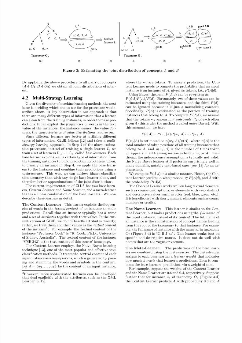
In summary, we estimate the joint probability distribu-tion of A and B as follows (the procedure is illustrated inFigure 3):

1. Partition U 1, into U A1 and U A1 , the set of instances thatdo and do not belong to A, respectively (Figures 3.a-b).

2. Train a learner L for instances of A, using U A1 and U A1as the sets of positive and negative training examples,respectively.

3. Partition U 2, the set of instances of taxonomy O2, intoU B2 and U B2 , the set of instances that do and do notbelong to B , respectively (Figures 3.d-e).

4. Apply learner L to each instance in U B2 (Figure 3.e).

This partitions U B2 into the two sets U A,B2 and U A,B2

shown in Figure 3.f. Similarly, applying L to U B2 re-

sults in the two sets U A,B2 and U A,B2 .

5. Repeat Steps 1-4, but with the roles of taxonomies O1

and O2 being reversed, to obtain the sets U A,B1 , U A,B1 ,

U A,B1 , and U A,B1 .

6. Finally, compute P (A, B) using Formula 3. The re-

maining three joint probabilities are computed in asimilar manner, using the sets U A,B2 , . . . , U A,B1 com-puted in Steps 4-5.

1This is a standard assumption in machine learning andstatistics, and seems appropriate here, unless the availableinstances were generated in some unusual way.2Notice that N (U A,Bi )/N (U i) is also a reasonable approx-imation of P (A, B), but it is estimated based only on thedata of Oi. The estimation in (3) is likely to be more accu-rate because it is based on more data, namely, the data of both O1 and O2.



R

A C D

E F

G

B H

I Jt1, t2 t3, t4

t5 t6, t7t1, t2, t3, t4

t5, t6, t7

Trained

Learner L

s2, s3 s4

s1

s5, s6

s1, s2, s3, s4

s5, s6

L s1, s3 s2, s4

s5 s6

Taxonomy O 2

U2

U1

not A

not A,B

Taxonomy O 1

U2not B

U1A

U2B

U2A,not B

U2not A,not B

U2A,B

(b) (c) (d) (e) (f)(a)

Figure 3: Estimating the joint distribution of concepts A and B

By applying the above procedure to all pairs of conceptsA ∈ O1, B ∈ O2 we obtain all joint distributions of inter-est.

4.2 Multi-Strategy LearningGiven the diversity of machine learning methods, the next

issue is deciding which one to use for the procedure we de-scribed above. A key observation in our approach is thatthere are many different types of information that a learner

can glean from the training instances, in order to make pre-dictions. It can exploit the frequencies of words in the textvalue of the instances, the instance names , the value for-mats , the characteristics of value distributions , and so on.

Since different learners are better at utilizing differenttypes of information, GLUE follows [12] and takes a multi-strategy learning approach. In Step 2 of the above estima-tion procedure, instead of training a single learner L, wetrain a set of learners L1, . . . , Lk, called base learners . Eachbase learner exploits well a certain type of information fromthe training instances to build prediction hypotheses. Then,to classify an instance in Step 4, we apply the base learn-ers to the instance and combine their predictions using ameta-learner . This way, we can achieve higher classifica-tion accuracy than with any single base learner alone, andtherefore better approximations of the joint distributions.

The current implementation of GLUE has two base learn-ers, Content Learner and Name Learner , and a meta-learnerthat is a linear combination of the base learners. We nowdescribe these learners in detail.

The Content Learner: This learner exploits the frequen-cies of words in the textual content of an instance to makepredictions. Recall that an instance typically has a name and a set of attributes together with their values. In the cur-rent version of GLUE, we do not handle attributes directly;rather, we treat them and their values as the textual content of the instance3. For example, the textual content of theinstance “Professor Cook” is “R. Cook, Ph.D., Universityof Sidney, Australia”. The textual content of the instance

“CSE 342” is the text content of this course’ homepage.The Content Learner employs the Naive Bayes learning

technique [13], one of the most popular and effective textclassification methods. It treats the textual content of eachinput instance as a bag of tokens , which is generated by pars-ing and stemming the words and symbols in the content.Let d = {w1, . . . , wk} be the content of an input instance,

3However, more sophisticated learners can be developedthat deal explicitly with the attributes, such as the XMLLearner in [12].

where the wj are tokens. To make a prediction, the Con-tent Learner needs to compute the probability that an inputinstance is an instance of A, given its tokens, i.e., P (A|d).

Using Bayes’ theorem, P (A|d) can be rewritten asP (d|A)P (A)/P (d). Fortunately, two of these values can beestimated using the training instances, and the third, P (d),can be ignored because it is just a normalizing constant.Specifically, P (A) is estimated as the portion of traininginstances that belong to A. To compute P (d|A), we assume

that the tokens wj appear in d independently of each othergiven A (this is why the method is called naive Bayes). Withthis assumption, we have

P (d|A) = P (w1|A)P (w2|A) · · ·P (wk|A)

P (wj |A) is estimated as n(wj , A)/n(A), where n(A) is thetotal number of token positions of all training instances thatbelong to A, and n(wj , A) is the number of times tokenwj appears in all training instances belonging to A. Eventhough the independence assumption is typically not valid,the Naive Bayes learner still performs surprisingly well inmany domains, notably text-based ones (see [13] for an ex-planation).

We compute P (A|d) in a similar manner. Hence, the Con-tent Learner predicts A with probability P (A|d), and A withthe probability P (A|d).

The Content Learner works well on long textual elements,such as course descriptions, or elements with very distinctand descriptive values, such as color (red, blue, green, etc.).It is less effective with short, numeric elements such as coursenumbers or credits.

The Name Learner: This learner is similar to the Con-tent Learner, but makes predictions using the full name of the input instance, instead of its content . The full name of an instance is the concatenation of concept names leadingfrom the root of the taxonomy to that instance. For exam-ple, the full name of instance with the name s4 in taxonomyO2 (Figure 3.d) is “G B J s4”. This learner works best onspecific and descriptive names. It does not do well withnames that are too vague or vacuous.

The Meta-Learner: The predictions of the base learn-ers are combined using the meta-learner. The meta-learnerassigns to each base learner a learner weight that indicateshow much it trusts that learner’s predictions. Then it com-bines the base learners’ predictions via a weighted sum.

For example, suppose the weights of the Content Learnerand the Name Learner are 0.6 and 0.4, respectively. Supposefurther that for instance s4 of taxonomy O2 (Figure 3.d)the Content Learner predicts A with probability 0.8 and A



with probability 0.2, and the Name Learner predicts A withprobability 0.3 and A with probability 0.7. Then the Meta-Learner predicts A with probability 0.8 · 0.6 + 0.3 · 0.4 = 0.6and A with probability 0.2 · 0.6 + 0.7 · 0.4 = 0.4.

In the current GLUE system, the learner weights are setmanually, based on the characteristics of the base learnersand the taxonomies. However, they can also be set auto-matically using a machine learning approach called stacking [37, 34], as we have shown in [12].

5. RELAXATION LABELINGWe now describe the Relaxation Labeler , which takes the

similarity matrix from the Similarity Estimator , and searchesfor the mapping configuration that best satisfies the givendomain constraints and heuristic knowledge. We first de-scribe relaxation labeling, then discuss the domain const-raints and heuristic knowledge employed in our approach.

5.1 Relaxation LabelingRelaxation labeling is an efficient technique to solve the

problem of assigning labels to nodes of a graph, given a setof constraints. The key idea behind this approach is that thelabel of a node is typically influenced by the features of the node’s neighborhood in the graph. Examples of such featuresare the labels of the neighboring nodes, the percentage of nodes in the neighborhood that satisfy a certain criterion,and the fact that a certain constraint is satisfied or not.

Relaxation labeling exploits this observation. The influ-ence of a node’s neighborhood on its label is quantified usinga formula for the probability of each label as a function of the neighborhood features. Relaxation labeling assigns ini-tial labels to nodes based solely on the intrinsic propertiesof the nodes. Then it performs iterative local optimization .In each iteration it uses the formula to change the label of a node based on the features of its neighborhood. This con-tinues until labels do not change from one iteration to thenext, or some other convergence criterion is reached.

Relaxation labeling appears promising for our purposesbecause it has been applied successfully to similar matchingproblems in computer vision, natural language processing,and hypertext classification [16, 31, 10]. It is relatively ef-ficient, and can handle a broad range of constraints. Eventhough its convergence properties are not yet well under-stood (except in certain cases) and it is liable to convergeto a local maxima, in practice it has been found to performquite well [31, 10].

We now explain how to apply relaxation labeling to theproblem of mapping from taxonomy O1 to taxonomy O2.We regard nodes (concepts) in O2 as labels , and recast the

problem as finding the best label assignment to nodes (con-cepts) in O1, given all knowledge we have about the domainand the two taxonomies.

Our goal is to derive a formula for updating the proba-bility that a node takes a label based on the features of theneighborhood. Let X be a node in taxonomy O1, and Lbe a label (i.e., a node in O2). Let ∆K represent all thatwe know about the domain, namely, the tree structures of the two taxonomies, the sets of instances, and the set of do-main constraints. Then we have the following conditionalprobability

0

0.1

0.2

0.3

0.4

0.5

0.6

0.7

0.8

0.9

1

-10 -5 0 5 10

P ( x )

x

Sigmoid(x)

Figure 4: The sigmoid function

P (X = L|∆K) =M X

P (X = L, M X |∆K)

= M X

P (X = L|M X , ∆K)P (M X |∆K) (4)

where the sum is over all possible label assignments M X toall nodes other than X in taxonomy O1. Assuming thatthe nodes’ label assignments are independent of each othergiven ∆K , we have

P (M X |∆K) =

(Xi=Li)∈M X

P (X i = Li|∆K) (5)

Consider P (X = L|M X , ∆K). M X and ∆K constitutesall that we know about the neighborhood of X . Supposenow that the probability of X getting label L depends onlyon the values of n features of this neighborhood, where eachfeature is a function f i(M X , ∆K , X , L). As we explain later

in this section, each such feature corresponds to one of theheuristics or domain constraints that we wish to exploit.Then

P (X = L|M X , ∆K) = P (X = L|f 1, . . . , f n) (6)

If we have access to previously-computed mappings be-tween taxonomies in the same domain, we can use them asthe training data from which to estimate P (X = L|f 1, . . . , f n)(see [10] for an example of this in the context of hypertextclassification). However, here we will assume that such map-pings are not available. Hence we use alternative methodsto quantify the influence of the features on the label assign-ment. In particular, we use the sigmoid or logistic functionσ(x) = 1/(1 + e−x), where x is a linear combination of thefeatures f k, to estimate the above probability. This functionis widely used to combine multiple sources of evidence [5].The general shape of the sigmoid is as shown in Figure 4.

Thus:

P (X = L|f 1, . . . , f n) ∝ σ(α1 · f 1 + · · · + αn · f n) (7)

where ∝ denotes “proportional to”, and the weight αk indi-cates the importance of feature f k.

The sigmoid is essentially a smoothed threshold function,which makes it a good candidate for use in combining ev-idence from the different features. If the total evidence is



Constraint Types Examples

Neighborhood

Two nodes match if their children also match.

Two nodes match if their parents match and at least x% of their children also match.

Two nodes match if their parents match and some of their descendants also match.

Domain-

Independent

Union If all children of node X match node Y, then X also matches Y.

SubsumptionIf node Y is a descendant of node X, and Y matches PROFESSOR, then itis unlikely that X matches ASST PROFESSOR.

If node Y is NOT a descendant of node X, and Y matches PROFESSOR, then it is unlikely that X matches FACULTY.

Frequency There can be at most one node that matches DEPARTMENT CHAIR.

Domain-Depen

dent

NearbyIf a node in the neighborhood of node X matches ASSOC PROFESSOR, then the chance thatX matches PROFESSOR is

increased.

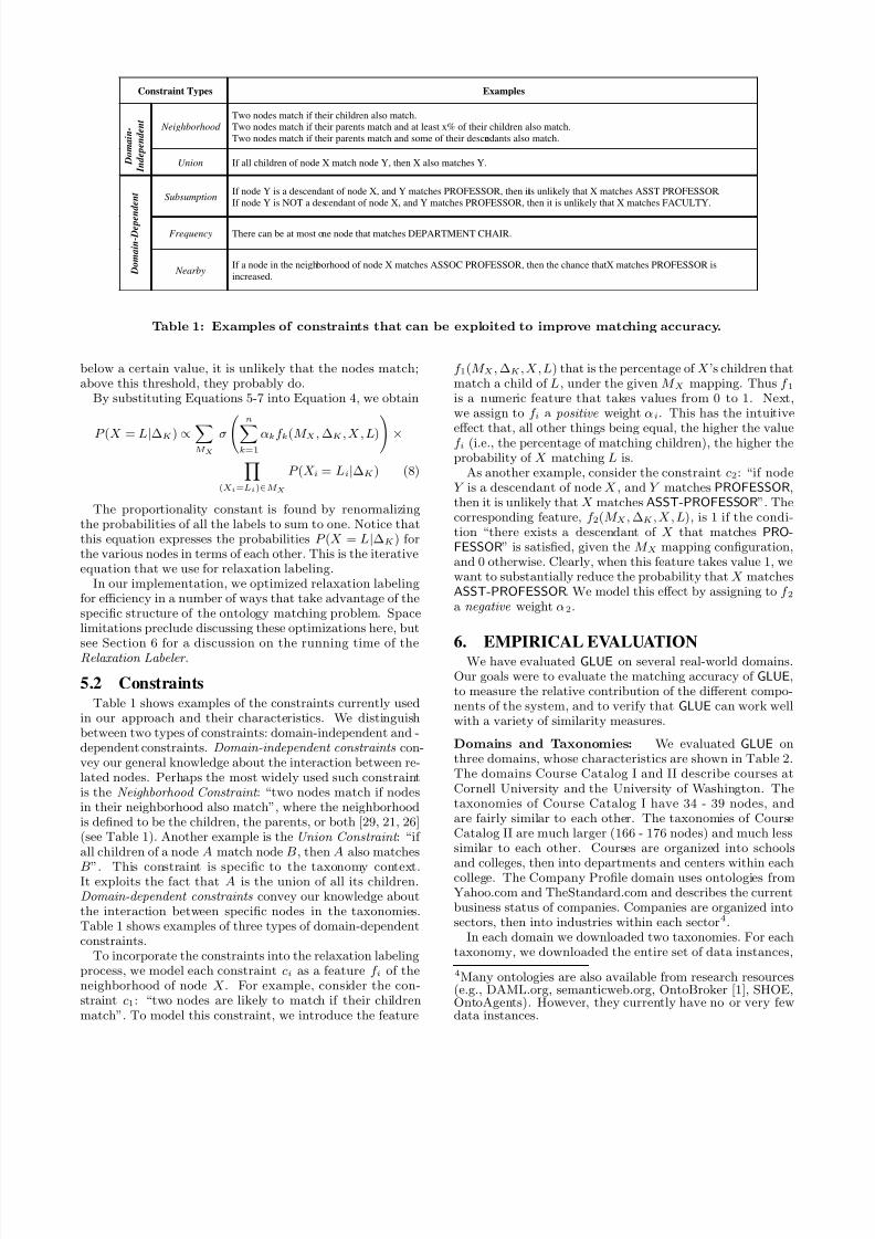
Table 1: Examples of constraints that can be exploited to improve matching accuracy.

below a certain value, it is unlikely that the nodes match;above this threshold, they probably do.

By substituting Equations 5-7 into Equation 4, we obtain

P (X = L|∆K) ∝M X

σ nk=1

αkf k(M X , ∆K , X , L)×

(Xi=Li)∈M X

P (X i = Li|∆K) (8)

The proportionality constant is found by renormalizingthe probabilities of all the labels to sum to one. Notice thatthis equation expresses the probabilities P (X = L|∆K) forthe various nodes in terms of each other. This is the iterativeequation that we use for relaxation labeling.

In our implementation, we optimized relaxation labelingfor efficiency in a number of ways that take advantage of thespecific structure of the ontology matching problem. Spacelimitations preclude discussing these optimizations here, butsee Section 6 for a discussion on the running time of theRelaxation Labeler .

5.2 ConstraintsTable 1 shows examples of the constraints currently used

in our approach and their characteristics. We distinguishbetween two types of constraints: domain-independent and -dependent constraints. Domain-independent constraints con-vey our general knowledge about the interaction between re-lated nodes. Perhaps the most widely used such constraintis the Neighborhood Constraint : “two nodes match if nodesin their neighborhood also match”, where the neighborhoodis defined to be the children, the parents, or both [29, 21, 26](see Table 1). Another example is the Union Constraint : “if all children of a node A match node B , then A also matches

B”. This constraint is specific to the taxonomy context.It exploits the fact that A is the union of all its children.Domain-dependent constraints convey our knowledge aboutthe interaction between specific nodes in the taxonomies.Table 1 shows examples of three types of domain-dependentconstraints.

To incorporate the constraints into the relaxation labelingprocess, we model each constraint ci as a feature f i of theneighborhood of node X . For example, consider the con-straint c1: “two nodes are likely to match if their childrenmatch”. To model this constraint, we introduce the feature

f 1(M X , ∆K , X , L) that is the percentage of X ’s children thatmatch a child of L, under the given M X mapping. Thus f 1is a numeric feature that takes values from 0 to 1. Next,we assign to f i a positive weight αi. This has the intuitive

effect that, all other things being equal, the higher the valuef i (i.e., the percentage of matching children), the higher theprobability of X matching L is.

As another example, consider the constraint c2: “if nodeY is a descendant of node X , and Y matches PROFESSOR,then it is unlikely that X matches ASST-PROFESSOR”. Thecorresponding feature, f 2(M X , ∆K , X , L), is 1 if the condi-tion “there exists a descendant of X that matches PRO-FESSOR” is satisfied, given the M X mapping configuration,and 0 otherwise. Clearly, when this feature takes value 1, wewant to substantially reduce the probability that X matchesASST-PROFESSOR. We model this effect by assigning to f 2a negative weight α2.

6. EMPIRICAL EVALUATIONWe have evaluated GLUE on several real-world domains.

Our goals were to evaluate the matching accuracy of GLUE,to measure the relative contribution of the different compo-nents of the system, and to verify that GLUE can work wellwith a variety of similarity measures.

Domains and Taxonomies: We evaluated GLUE onthree domains, whose characteristics are shown in Table 2.The domains Course Catalog I and II describe courses atCornell University and the University of Washington. Thetaxonomies of Course Catalog I have 34 - 39 nodes, andare fairly similar to each other. The taxonomies of CourseCatalog II are much larger (166 - 176 nodes) and much lesssimilar to each other. Courses are organized into schools

and colleges, then into departments and centers within eachcollege. The Company Profile domain uses ontologies fromYahoo.com and TheStandard.com and describes the currentbusiness status of companies. Companies are organized intosectors, then into industries within each sector4.

In each domain we downloaded two taxonomies. For eachtaxonomy, we downloaded the entire set of data instances,

4Many ontologies are also available from research resources(e.g., DAML.org, semanticweb.org, OntoBroker [1], SHOE,OntoAgents). However, they currently have no or very fewdata instances.



Taxonomies # nodes# non -leaf

nodesdepth

# instances

in

taxonomy

max # instances

at a leaf

max #

children

of a node

# manual

mappings

created

Cornell 34 6 4 1526 155 10 34Course Catalog

I Washington 39 8 4 1912 214 11 37

Cornell 176 27 4 4360 161 27 54Course Catalog

II Washington 166 25 4 6957 214 49 50

Standard.com 333 30 3 13634 222 29 236Company

Profiles Yahoo.com 115 13 3 9504 656 25 104

Table 2: Domains and taxonomies for our experiments.

0

10

20

30

40

50

60

70

80

90

100

Cornell to Wash. Wash. to Cornell Cornell to Wash. Wash. to Cornell Standard to Yahoo Yahoo to Standard

Matchingaccuracy(%)

Name Learner Content Learner Meta Learner Relaxation Labeler

Course Catalog II Company ProfileCourse Catalog I

Figure 5: Matching accuracy of GLUE.

and performed some trivial data cleaning such as removingHTML tags and phrases such as “course not offered” fromthe instances. We also removed instances of size less than130 bytes, because they tend to be empty or vacuous, andthus do not contribute to the matching process. We thenremoved all nodes with fewer than 5 instances, because suchnodes cannot be matched reliably due to lack of data.

Similarity Measure & Manual Mappings: We choseto evaluate GLUE using the Jaccard similarity measure (Sec-tion 3), because it corresponds well to our intuitive under-standing of similarity. Given the similarity measure, wemanually created the correct 1-1 mappings between the tax-onomies in the same domain, for evaluation purposes. Therightmost column of Table 2 shows the number of manualmappings created for each taxonomy. For example, we cre-ated 236 one-to-one mappings from Standard to Yahoo! , and104 mappings in the reverse direction. Note that in somecases there were nodes in a taxonomy for which we couldnot find a 1-1 match. This was either because there wasno equivalent node (e.g., School of Hotel Administration atCornell has no equivalent counterpart at the University of Washington), or when it is impossible to determine an ac-curate match without additional domain expertise.

Domain Constraints: We specified domain constraintsfor the relaxation labeler. For the taxonomies in Course Cat-alog I, we specified all applicable subsumption constraints(see Table 1). For the other two domains, because theirsheer size makes specifying all constraints difficult, we spec-ified only the most obvious subsumption constraints (about10 constraints for each taxonomy). For the taxonomies inCompany Profiles we also used several frequency constraints.

Experiments: For each domain, we performed two ex-periments. In each experiment, we applied GLUE to findthe mappings from one taxonomy to the other. The match-ing accuracy of a taxonomy is then the percentage of themanual mappings (for that taxonomy) that GLUE predictedcorrectly.

6.1 Matching AccuracyFigure 5 shows the matching accuracy for different do-

mains and configurations of GLUE. In each domain, we showthe matching accuracy of two scenarios: mapping from thefirst taxonomy to the second, and vice versa. The four barsin each scenario (from left to right) represent the accuracyproduced by: (1) the name learner alone, (2) the contentlearner alone, (3) the meta-learner using the previous twolearners, and (4) the relaxation labeler on top of the meta-learner (i.e., the complete GLUE system).

The results show that GLUE achieves high accuracy acrossall three domains, ranging from 66 to 97%. In contrast, thebest matching results of the base learners, achieved by thecontent learner, are only 52 - 83%. It is interesting that thename learner achieves very low accuracy, 12 - 15% in four out

of six scenarios. This is because all instances of a concept,say B, have very similar full names (see the description of thename learner in Section 4.2). Hence, when the name learnerfor a concept A is applied to B , it will classify al l instancesof B as A or A. In cases when this classfication is incorrect,which might be quite often, using the name learner aloneleads to poor estimates of the joint distributions. The poorperformance of the name learner underscores the importanceof data instances and multi-strategy learning in ontologymatching.

The results clearly show the utility of the meta-learner and



relaxation labeler. Even though in half of the cases the meta-learner only minimally improves the accuracy, in the otherhalf it makes substantial gains, b etween 6 and 15%. Andin all but one case, the relaxation labeler further improvesaccuracy by 3 - 18%, confirming that it is able to exploitthe domain constraints and general heuristics. In one case(from Standard to Yahoo), the relaxation labeler decreasedaccuracy by 2%. The performance of the relaxation labeler isdiscussed in more detail below. In Section 6.4 we identify the

reasons that prevent GLUE from identifying the remainingmappings.

In the current experiments, GLUE utilized on average only30 to 90 data instances per leaf node (see Table 2). The highaccuracy in these experiments suggests that GLUE can workwell with only a modest amount of data.

6.2 Performance of the Relaxation LabelerIn our experiments, when the relaxation labeler was ap-

plied, the accuracy typically improved substantially in thefirst few iterations, then gradually dropped. This phenomenonhas also been observed in many previous works on relaxationlabeling [16, 20, 31]. Because of this, finding the right stop-ping criterion for relaxation labeling is of crucial importance.

Many stopping criteria have been proposed, but no generaleffective criterion has been found.We considered three stopping criteria: (1) stopping when

the mappings in two consecutive iterations do not change(the mapping criterion ), (2) when the probabilities do notchange, or (3) when a fixed number of iterations has beenreached.

We observed that when using the last two criteria the ac-curacy sometimes improved by as much as 10%, but most of the time it decreased. In contrast, when using the mappingcriterion, in all but one of our experiments the accuracy sub-stantially improved, by 3 - 18%, and hence, our results arereported using this criterion. We note that with the map-ping criterion, we observed that relaxation labeling alwaysstopped in the first few iterations.

In all of our experiments, relaxation labeling was also veryfast. It took only a few seconds in Catalog I and under 20seconds in the other two domains to finish ten iterations.This observation shows that relaxation labeling can be im-plemented efficiently in the ontology-matching context. Italso suggests that we can efficiently incorporate user feed-back into the relaxation labeling process in the form of ad-ditional domain constraints.

We also experimented with different values for the con-straint weights (see Section 5), and found that the relax-ation labeler was quite robust with respect to such parame-ter changes.

6.3 Most-Specific-Parent Similarity Measure

So far we have experimented only with the Jaccard simi-larity measure. We wanted to know whether GLUE can workwell with other similarity measures. Hence we conducted anexperiment in which we used GLUE to find mappings for tax-onomies in the Course Catalog I domain, using the followingsimilarity measure:

MSP (A, B) =

P (A|B) if P (B|A) ≥ 1 −

0 otherwise

This measure is the same as the the most-specific-parent similarity measure described in Section 3, except that we

0

10

20

30

40

50

60

70

80

90

100

0 0.1 0.2 0.3 0.4 0.5

MatchingAccura

cy(%)

Cornell to Wash. Wash. To Cornell

Epsilon

Figure 6: The accuracy of GLUE in the Course Cat-

alog I domain, using the most-specific-parent simi-

larity measure.

added an factor to account for the error in approximatingP (B|A).

Figure 6 shows the matching accuracy, plotted against .As can be seen, GLUE performed quite well on a broad rangeof . This illustrates how GLUE can be effective with morethan one similarity measure.

6.4 DiscussionThe accuracy of GLUE is quite impressive as is, but it is

natural to ask what limits GLUE from obtaining even higheraccuracy. There are several reasons that prevent GLUE fromcorrectly matching the remaining nodes. First, some nodescannot be matched because of insufficient training data. Forexample, many course descriptions in Course Catalog II con-tain only vacuous phrases such as “3 credits”. While thereis clearly no general solution to this problem, in many casesit can be mitigated by adding base learners that can exploitdomain characteristics to improve matching accuracy. Andsecond, the relaxation labeler performed local optimizations,and sometimes converged to only a local maxima, therebynot finding correct mappings for all nodes. Here, the chal-lenge will be in developing search techniques that work bet-ter by taking a more “global perspective”, but still retainthe runtime efficiency of local optimization. Further, thetwo base learners we used in our implementation are rathersimple general-purpose text classifiers. Using other leaners

that perform domain-specific feature selection and compar-ison can also improve the accuracy.

We note that some nodes cannot be matched automati-cally because they are simply ambiguous. For example, itis not clear whether “networking and communication de-vices” should match “communication equipment” or “com-puter networks”. A solution to this problem is to incorpo-rate user interaction into the matching process [28, 12, 38].

GLUE currently tries to predict the best match for every node in the taxonomy. However, in some cases, such a matchsimply does not exist (e.g., unlike Cornell, the University of



Washington does not have a School of Hotel Administra-tion). Hence, an additional extension to GLUE is to make itbe aware of such cases, and not predict an incorrect matchwhen this occurs.

7. RELATED WORKGLUE is related to our previous work on LSD [12], whose

goal was to semi-automatically find schema mappings for

data integration. There, we had a mediated schema, andour goal was to find mappings from the schemas of a multi-tude of data sources to the mediated schema. The observa-tion was that we can use a set of manually given mappingson several sources as training examples for a learner thatpredicts mappings for subsequent sources. LSD illustratedthe effectiveness of multi-strategy learning for this problem.In GLUE since our problem is to match a pair of ontologies,there are no manual mappings for training, and we need toobtain the training examples for the learner automatically.Further, since GLUE deals with a more expressive formalism(ontologies versus schemas), the role of constraints is muchmore important, and we innovate by using relaxation label-ing for this purpose. Finally, LSD did not consider in depththe semantics of a mapping, as we do here.

We now describe other related work to GLUE from severalperspectives.

Ontology Matching: Many works have addressed on-tology matching in the context of ontology design and in-tegration (e.g., [11, 24, 28, 27]). These works do not dealwith explicit notions of similarity. They use a variety of heuristics to match ontology elements. They do not use ma-chine learning and do not exploit information in the datainstances. However, many of them [24, 28] have powerfulfeatures that allow for efficient user interaction, or expres-sive rule languages [11] for specifying mappings. Such fea-tures are important components of a comprehensive solutionto ontology matching, and hence should be added to GLUEin the future.

Several recent works have attempted to further automatethe ontology matching process. The Anchor-PROMPT sys-tem [29] exploits the general heuristic that paths (in thetaxonomies or ontology graphs) between matching elementstend to contain other matching elements. The HICAL sys-tem [17] exploits the data instances in the overlap betweenthe two taxonomies to infer mappings. [18] computes thesimilarity between two taxonomic nodes based on their sig-nature TF/IDF vectors, which are computed from the datainstances.

Schema Matching: Schemas can be viewed as ontologieswith restricted relationship types. The problem of schemamatching has been studied in the context of data integra-tion and data translation (see [33] for a survey). Severalworks [26, 21, 25] have exploited variations of the generalheuristic “two nodes match if nodes in their neighborhoodalso match”, but in an isolated fashion, and not in the samegeneral framework we have in GLUE.

Notions of Similarity: The similarity measure in [17] isbased on κ statistics, and can be thought of as being definedover the joint probability distribution of the concepts in-volved. In [19] the authors propose an information-theoreticnotion of similarity that is based on the joint distribution.These works argue for a single best universal similarity mea-

sure, whereas GLUE allows for application-dependent simi-larity measures.

Ontology Learning: Machine learning has been appliedto other ontology-related tasks, most notably learning toconstruct ontologies from data and other ontologies, andextracting ontology instances from data [30, 23, 32]. Ourwork here provides techniques to help in the ontology con-struction process [23]. [22] gives a comprehensive summary

of the role of machine learning in the Semantic Web effort.

8. CONCLUSION AND FUTURE WORKThe vision of the Semantic Web is grand. With the prolif-

eration of ontologies on the Semantic Web, the developmentof automated techniques for ontology matching will be cru-cial to its success.

We have described an approach that applies machine learn-ing techniques to propose such semantic mappings. Ourapproach is based on well-founded notions of semantic sim-ilarity, expressed in terms of the joint probability distribu-tion of the concepts involved. We described the use of ma-chine learning, and in particular, of multi-strategy learning,for computing concept similarities. This learning technique

makes our approach easily extensible to additional learn-ers, and hence to exploiting additional kinds of knowledgeabout instances. Finally, we introduced relaxation labelingto the ontology-matching context, and showed that it can beadapted to efficiently exploit a variety of heuristic knowledgeand domain-specific constraints to further improve matchingaccuracy. Our experiments showed that we can accuratelymatch 66 - 97% of the nodes on several real-world domains.

Aside from striving to improve the accuracy of our meth-ods, our main line of future research involves extending ourtechniques to handle more sophisticated mappings betweenontologies (i.e., non 1-1 mappings), and exploiting more of the constraints that are expressed in the ontologies (viaattributes and relationships, and constraints expressed onthem).

Acknowledgments

We thank Phil Bernstein, Geoff Hulten, Natasha Noy, RachelPottinger, Matt Richardson, Pradeep Shenoy, and the anony-mous reviewers for their invaluable comments. This work issupported by NSF Grants 9523649, 9983932, IIS-9978567,and IIS-9985114. The third author is also supported by anIBM Faculty Partnership Award. The fourth author is alsosupported by a Sloan Fellowship and gifts from MicrosoftResearch, NEC and NTT.

9. REFERENCES

[1] http://ontobroker.semanticweb.org.[2] www.daml.org.

[3] www.google.com.

[4] IEEE Intelligent Systems , 16(2), 2001.

[5] A. Agresti. Categorical Data Analysis . Wiley, NewYork, NY, 1990.

[6] T. Berners-Lee, J. Hendler, and O. Lassila. The Seman-tic Web. Scientific American , 279, 2001.

[7] D. Brickley and R. Guha. Resource Description Frame-work Schema Specification 1.0, 2000.



[8] J. Broekstra, M. Klein, S. Decker, D. Fensel, F. vanHarmelen, and I. Horrocks. Enabling knowledge rep-resentation on the Web by Extending RDF Schema.In Proceedings of the Tenth International World Wide Web Conference , 2001.

[9] D. Calvanese, D. G. Giuseppe, and M. Lenzerini. Ontol-ogy of Integration and Integration of Ontologies. In Pro-ceedings of the 2001 Description Logic Workshop (DL2001).

[10] S. Chakrabarti, B. Dom, and P. Indyk. Enhanced Hy-pertext Categorization Using Hyperlinks. In Proceed-ings of the ACM SIGMOD Conference , 1998.

[11] H. Chalupsky. Ontomorph: A Translation system forsymbolic knowledge. In Principles of Knowledge Rep-resentation and Reasoning , 2000.

[12] A. Doan, P. Domingos, and A. Halevy. ReconcilingSchemas of Disparate Data Sources: A Machine Learn-ing Approach. In Proceedings of the ACM SIGMOD Conference , 2001.

[13] P. Domingos and M. Pazzani. On the Optimality of theSimple Bayesian Classifier under Zero-One Loss. Ma-chine Learning , 29:103–130, 1997.

[14] D. Fensel. Ontologies: Silver Bullet for Knowl-

edge Management and Electronic Commerce . Springer-Verlag, 2001.

[15] J. Heflin and J. Hendler. A Portrait of the SemanticWeb in Action. IEEE Intelligent Systems , 16(2), 2001.

[16] R. Hummel and S. Zucker. On the Foundations of Re-laxation Labeling Processes. PAMI , 5(3):267–287, May1983.

[17] R. Ichise, H. Takeda, and S. Honiden. Rule Inductionfor Concept Hierarchy Alignment. In Proceedings of the Workshop on Ontology Learning at the 17th Interna-tional Joint Conference on Artificial Intelligence (IJ-CAI), 2001.

[18] M. Lacher and G. Groh. Facilitating the exchange of explixit knowledge through ontology mappings. In Pro-

ceedings of the 14th Int. FLAIRS conference , 2001.[19] D. Lin. An Information-Theoritic Definiton of Similar-

ity. In Proceedings of the International Conference on Machine Learning (ICML), 1998.

[20] S. Lloyd. An optimization approach to relaxation la-beling algorithms. Image and Vision Computing , 1(2),1983.

[21] J. Madhavan, P. Bernstein, and E. Rahm. GenericSchema Matching with Cupid. In Proceedings of the International Conference on Very Large Databases (VLDB), 2001.

[22] A. Maedche. A Machine Learning Perspective for theSemantic Web. Semantic Web Working Symposium(SWWS) Position Paper, 2001.

[23] A. Maedche and S. Saab. Ontology Learning for theSemantic Web. IEEE Intelligent Systems , 16(2), 2001.

[24] D. McGuinness, R. Fikes, J. Rice, and S. Wilder.The Chimaera Ontology Environment. In Proceedings of the 17th National Conference on Artificial Intelli-gence (AAAI), 2000.

[25] S. Melnik, H. Molina-Garcia, and E. Rahm. Similar-ity Flooding: A Versatile Graph Matching Algorithm.In Proceedings of the International Conference on Data Engineering (ICDE), 2002.

[26] T. Milo and S. Zohar. Using Schema Matching to Sim-plify Heterogeneous Data Translation. In Proceedings of the International Conference on Very Large Databases (VLDB), 1998.

[27] P. Mitra, G. Wiederhold, and J. Jannink. Semi-automatic Integration of Knowledge Sources. In Pro-ceedings of Fusion’99 .

[28] N. Noy and M. Musen. PROMPT: Algorithm and Toolfor Automated Ontology Merging and Alignment. InProceedings of the National Conference on Artificial In-telligence (AAAI), 2000.

[29] N. Noy and M. Musen. Anchor-PROMPT: Using Non-Local Context for Semantic Matching. In Proceedings of the Workshop on Ontologies and Information Shar-ing at the International Joint Conference on Artificial

Intelligence (IJCAI), 2001.[30] B. Omelayenko. Learning of Ontologies for the Web:

the Analysis of Existent approaches. In Proceedings of the International Workshop on Web Dynamics , 2001.

[31] L. Padro. A Hybrid Environment for Syntax-SemanticTagging, 1998.

[32] N. Pernelle, M.-C. Rousset, and V. Ventos. AutomaticConstruction and Refinement of a Class Hierarchy overSemi-Structured Data. In Proceeding of the Workshopon Ontology Learning at the 17th International Joint Conference on Artificial Intelligence (IJCAI), 2001.

[33] E. Rahm and P. Bernstein. On Matching Schemas Au-tomatically. VLDB Journal , 10(4), 2001.

[34] K. M. Ting and I. H. Witten. Issues in stacked gen-

eralization. Journal of Artificial Intelligence Research (JAIR), 10:271–289, 1999.

[35] M. Uschold. Where is the semantics in the Seman-tic Web? In Workshop on Ontologies in Agent Sys-tems (OAS) at the 5th International Conference on Au-tonomous Agents , 2001.

[36] van Rijsbergen. Information Retrieval . Lon-don:Butterworths, 1979. Second Edition.

[37] D. Wolpert. Stacked generalization. Neural Networks ,5:241–259, 1992.

[38] L. Yan, R. Miller, L. Haas, and R. Fagin. Data DrivenUnderstanding and Refinement of Schema Mappings.In Proceedings of the ACM SIGMOD , 2001.

Learning to Map between Ontologies.pdf

Documents

Transcript of Learning to Map between Ontologies.pdf