Learning to Learn Graph Topologies

Xingyue Pu

University of Oxfordxpu@robots.ox.ac.uk

Tianyue Cao Xiaoyun Zhang

Shanghai Jiao Tong University{vanessa_,xiaoyun.zhang}@sjtu.edu.cn

Xiaowen Dong

University of Oxfordxdong@robots.ox.ac.uk

Siheng Chen⇤

Shanghai Jiao Tong Universitysihengc@sjtu.edu.cn

Abstract

Learning a graph topology to reveal the underlying relationship between dataentities plays an important role in various machine learning and data analysistasks. Under the assumption that structured data vary smoothly over a graph, theproblem can be formulated as a regularised convex optimisation over a positivesemidefinite cone and solved by iterative algorithms. Classic methods require anexplicit convex function to reflect generic topological priors, e.g. the `1 penaltyfor enforcing sparsity, which limits the flexibility and expressiveness in learningrich topological structures. We propose to learn a mapping from node data to thegraph structure based on the idea of learning to optimise (L2O). Specifically, ourmodel first unrolls an iterative primal-dual splitting algorithm into a neural network.The key structural proximal projection is replaced with a variational autoencoderthat refines the estimated graph with enhanced topological properties. The modelis trained in an end-to-end fashion with pairs of node data and graph samples.Experiments on both synthetic and real-world data demonstrate that our model ismore efficient than classic iterative algorithms in learning a graph with specifictopological properties.

1 Introduction

Graphs are an effective modelling language for revealing relational structure in high-dimensionalcomplex domains and may assist in a variety of machine learning tasks. However, in many practicalscenarios an explicit graph structure may not be readily available or easy to define. Graph learningaims at learning a graph topology from observation on data entities and is therefore an importantproblem studied in the literature.

Model-based graph learning from the perspectives of probabilistic graphical models [24] or graphsignal processing [32, 30, 28] solves an optimisation problem over the space of graph candidateswhose objective function reflects the inductive graph-data interactions. The data are referred as to theobservations on nodes, node features or graph signals in literature. The convex objective functionoften contains a graph-data fidelity term and a structural regulariser. For example, by assuming thatdata follow a multivariate Gaussian distribution, the graphical Lasso [2] maximises the `1 regularisedlog-likelihood of the precision matrix which corresponds to a conditional independence graph. Basedon the convex formulation, the problem of learning an optimal graph can be solved by many iterativealgorithms, such as proximal gradient descent [15], with convergence guarantees.

These classical graph learning approaches, despite being effective, share several common limita-tions. Firstly, handcrafted convex regularisers may not be expressive enough for representing the

⇤Corresponding author

35th Conference on Neural Information Processing Systems (NeurIPS 2021).

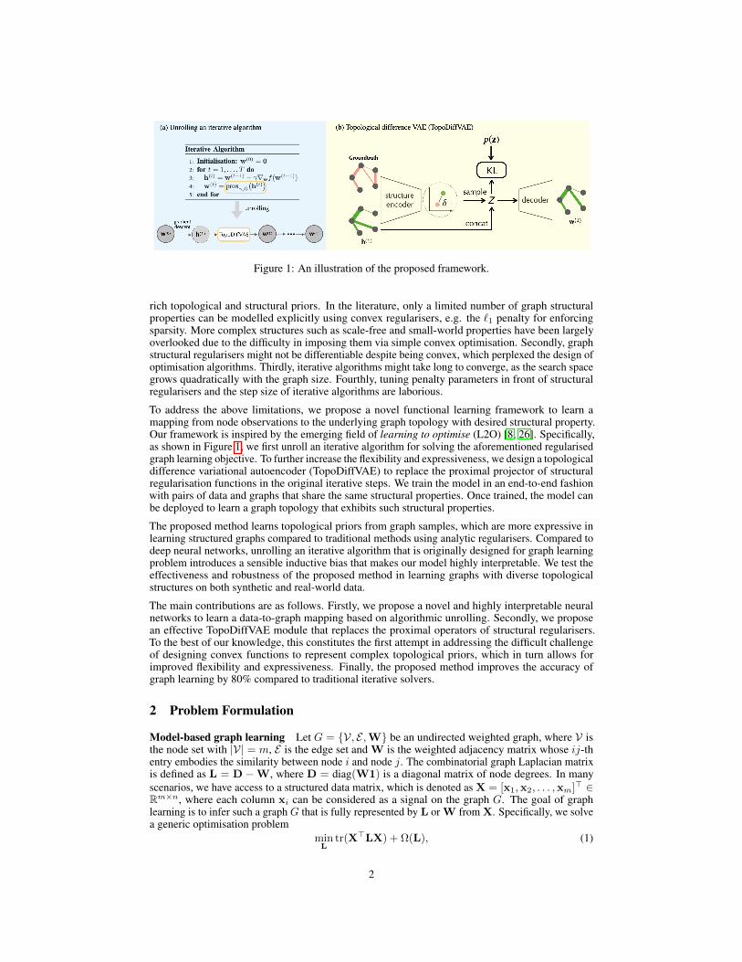
Figure 1: An illustration of the proposed framework.

rich topological and structural priors. In the literature, only a limited number of graph structuralproperties can be modelled explicitly using convex regularisers, e.g. the `1 penalty for enforcingsparsity. More complex structures such as scale-free and small-world properties have been largelyoverlooked due to the difficulty in imposing them via simple convex optimisation. Secondly, graphstructural regularisers might not be differentiable despite being convex, which perplexed the design ofoptimisation algorithms. Thirdly, iterative algorithms might take long to converge, as the search spacegrows quadratically with the graph size. Fourthly, tuning penalty parameters in front of structuralregularisers and the step size of iterative algorithms are laborious.

To address the above limitations, we propose a novel functional learning framework to learn amapping from node observations to the underlying graph topology with desired structural property.Our framework is inspired by the emerging field of learning to optimise (L2O) [8, 26]. Specifically,as shown in Figure 1, we first unroll an iterative algorithm for solving the aforementioned regularisedgraph learning objective. To further increase the flexibility and expressiveness, we design a topologicaldifference variational autoencoder (TopoDiffVAE) to replace the proximal projector of structuralregularisation functions in the original iterative steps. We train the model in an end-to-end fashionwith pairs of data and graphs that share the same structural properties. Once trained, the model canbe deployed to learn a graph topology that exhibits such structural properties.

The proposed method learns topological priors from graph samples, which are more expressive inlearning structured graphs compared to traditional methods using analytic regularisers. Compared todeep neural networks, unrolling an iterative algorithm that is originally designed for graph learningproblem introduces a sensible inductive bias that makes our model highly interpretable. We test theeffectiveness and robustness of the proposed method in learning graphs with diverse topologicalstructures on both synthetic and real-world data.

The main contributions are as follows. Firstly, we propose a novel and highly interpretable neuralnetworks to learn a data-to-graph mapping based on algorithmic unrolling. Secondly, we proposean effective TopoDiffVAE module that replaces the proximal operators of structural regularisers.To the best of our knowledge, this constitutes the first attempt in addressing the difficult challengeof designing convex functions to represent complex topological priors, which in turn allows forimproved flexibility and expressiveness. Finally, the proposed method improves the accuracy ofgraph learning by 80% compared to traditional iterative solvers.

2 Problem Formulation

Model-based graph learning Let G = {V, E ,W} be an undirected weighted graph, where V isthe node set with |V| = m, E is the edge set and W is the weighted adjacency matrix whose ij-thentry embodies the similarity between node i and node j. The combinatorial graph Laplacian matrixis defined as L = D �W, where D = diag(W1) is a diagonal matrix of node degrees. In manyscenarios, we have access to a structured data matrix, which is denoted as X = [x1,x2, . . . ,xm]> 2Rm⇥n, where each column xi can be considered as a signal on the graph G. The goal of graphlearning is to infer such a graph G that is fully represented by L or W from X. Specifically, we solvea generic optimisation problem

minL

tr(X>LX) + ⌦(L), (1)

2

where the first term is the so-called Laplacian quadratic form, measuring the variation of X on thegraph, and ⌦(L) is a convex regulariser on L to reflect structural priors. Since W is symmetric,we introduce the vector of edge weights w 2 Rm(m�1)/2

+ and reparameterise Eq.(1) based ontr(X>

LX) =P

i,j Wij ||xi � xj ||22 = 2w>y, where y 2 Rm(m�1)/2

+ is the half-vectorisation ofthe Euclidean distance matrix. Now, we optimise the objective w.r.t w such that

minw

2w>y + I{w�0}(w) + ⌦1(w) + ⌦2(Dw), (2)

where I is an indicator function such that IC(w) = 0 if w 2 C and IC(w) = 1 otherwise, and Dis a linear operator that transforms w into the vector of node degrees such that Dw = W1. Thereparameterisation reduces the dimension of search space by a half and we do not need to take extracare of the positive semi-definiteness of L.

In Eq.(2), the regularisers ⌦ is split into ⌦1 and ⌦2 on edge weights and node degrees respectively.Both formulations can be connected to many previous works, where regularisers are mathematicallyhandcrafted to reflect specific graph topologies. For example, the `1-regularised log-likelihoodmaximisation of the precision matrix with Laplacian constraints [23, 22] can be seen as a special caseof Eq.(1), where ⌦(L) = log det(L+ �2

I) + �P

i 6=j |Lij |. The `1 norm on edge weights enforcesthe learned conditional independence graph to be sparse. The author in [16] considers the log-barrieron node degrees, i.e. ⌦2(Dw) = �1

> log(Dw), to prevent the learned graph with isolated nodes.Furthermore, ⌦1(w) = ||w||22 is often added to force the edge weights to be smooth [11, 16].

Learning to learn graph topologies In many real-world applications, the mathematically-designedtopological priors in the above works might not be expressive enough. For one thing, many interestingpriors are too complex to be abstracted as an explicit convex function, e.g. the small-world property[36]. Moreover, those constraints added to prevent trivial solutions might conflict with the underlyingstructure. For example, the aforementioned log barrier may encourage many nodes with a largedegree, which contradicts the power-law assumption in scale-free graphs. The penalty parameters,treated as a part of regularisation, are manually appointed or tuned from inadequately granularity,which may exacerbate the lack of topological expressiveness. These motivate us to directly learn thetopological priors from graphs.

Formally, we aim at learning a neural network F✓(·) that maps the data term y to a graph represen-tation w that share the same topological properties and hence belong to the same graph family G.With training pairs {(yi,wi)}ni=1, we consider a supervised learning framework to obtain optimalF⇤

✓ such that

✓⇤ = argmin✓

Ew⇠G [L(F✓(y),w)], (3)

where L(bw,w) is a loss surrogate between the estimation bw = F✓(y) and the groundtruth. Oncetrained, the optimal F⇤

✓ (·) implicitly carries topological priors and can be applied to estimate graphsfrom new observations. Therefore, our framework promotes learning to learn a graph topology. Inthe next section, we elaborate on the architecture of F✓(·) and the design of L(·, ·).

3 Unrolled Networks with Topological Enhancement

In summary, the data-to-graph mapping F✓(·) is modelled with unrolling layers (Section 3.1) inher-ited from a primal-dual splitting algorithm that is originally proposed to solve the model-based graphlearning. We replace the proximal operator with a trainable variational autoencoder (i.e. TopoD-iffVAE) that refines the graph estimation with structural enhancement in Section 3.2. The overallnetwork is trained in an end-to-end fashion with the loss function introduced in Section 3.3.

3.1 Unrolling primal-dual iterative algorithm

Our model leverages the inductive bias from model-based graph learning. Specifically, we consider aspecial case of the formulation in Eq. (2) such that

minw

2w>y + I{w�0}(w)� ↵1> log(Dw) + �||w||22 (4)

3

where ⌦1(w) = �||w||22 and ⌦2(Dw) = �↵1> log(Dw), both of which are mathematicallyhandcrafted topological priors. To solve this optimisation problem, we consider a forward-backward-forward primal-dual splitting algorithm (PDS) in Algorithm 1. The algorithm is specifically derivedfrom Algorithm 6 in [21] by the authors in [16]. In Algorithm 1, Step 3, 5 and 7 update theprimal variable that corresponds to w, while Step 4, 6 and 8 update the dual variable in relationto node degrees. The forward steps are equivalent to a gradient descent on the primal variable(Step 3 and 7) and a gradient ascent on the the dual variable (Step 4 and 8), both of which arederived from the differentiable terms in Eq.(4). The backward steps (Step 5 and 6) are proximalprojections that correspond to two non-differentiable topological regularisers, i.e. the non-negativeconstraints on w and the log barrier on node degrees in Eq.(4). The detailed derivations are attachedin Appendix A.2. It should be note that `1 norm that promotes sparsity is implicitly included, i.e.2w>

y = 2w>(y � �/2) + �||w||1 given w � 0. We choose to unroll PDS as the main networkarchitecture of F✓(·), since the separate update steps of primal and dual variables allow us to replaceof proximal operators that are derived from other priors.

Algorithm 1 PDSInput: y, �, ↵ and �.

1: Initialisation: w(0) = 0,v(0) = 0

2: while |w(t) �w(t�1)| > ✏ do

3: r(t)1 = w

(t)��(2�w(t)+2y+D>v(t))

4: r(t)2 = v

(t) + �Dw(t)

5: p(t)1 = prox�,⌦1

(r(t)1 ) = max{0, r(t)1 }

6: p(t)2 = prox�,⌦2

(r(t)2 ), where�prox�(t),⌦2

(r2)�i=

r2,i�p

r22,i+4↵�

2

7: q(t)1 = p

(t)1 � �(2�p(t)

1 +2y+D>p(t)2 )

8: q(t)2 = p

(t)2 + �Dp

(t)1

9: w(t+1) = w

(t) � r(t)1 + q

(t)1

10: v(t+1) = v

(t) � r(t)2 + q

(t)2

11: end while

12: return bw = w(T )

Algorithm 2 Unrolling Net (L2G)

Input: y, T , enhancement(t)2{TRUE, FALSE}1: Initialisation: w

(0) = 0,v(0) = 0

2: for t = 0, 1, . . . , T do

3: r(t)1 = w

(t)��(t)(2�(t)w

(t)+2y+D>v(t))

4: r(t)2 = v

(t) + �(t)Dw(t)

5: if enhancement(t)=TRUE,p(t)1 = TopoDiffVAE(r(t)1 );

else,p(t)1 = prox�,⌦1

(r(t)1 ) = max{0, r(t)1 }.6: p

(t)2 = prox�(t),⌦2

(r(t)2 ), where�prox�(t),⌦2

(r2)�i=

r2,i�p

r22,i+4↵(t)�(t)

2

7: q(t)1 = p

(t)1 ��(t)(2�(t)

p(t)1 +2y+D>

p(t)2 )

8: q(t)2 = p

(t)2 + �(t)Dp

(t)1

9: w(t+1) = w

(t) � r(t)1 + q

(t)1

10: v(t+1) = v

(t) � r(t)2 + q

(t)2

11: end for

12: return w(1),w(2), . . . ,w(T ) = bw

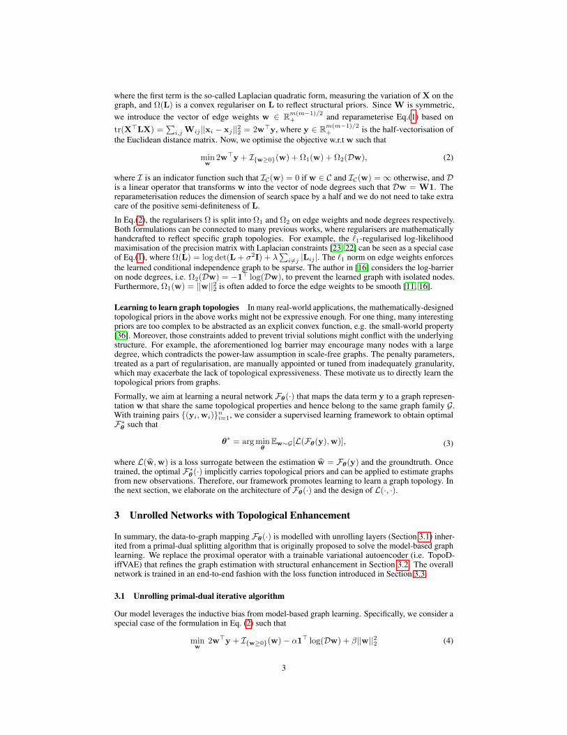
The proposed unrolling network is summarised in Algorithm 2, which unrolls the updating rules ofAlgorithm1 for T times and is hypothetically equivalent to running the iteration steps for T times. InAlgorithm 2, we consider two major substitutions to enable more flexible and expressive learning.

Firstly, we replace the hyperparameters ↵, � and the step size � in the PDS by layer-wise trainableparameters (highlighted in blue in Algorithm 2), which can be updated through backpropagation.Note that we consider independent trainable parameters in each unrolling layer, as we found it canenhance the representation capacity and boost the performance compared to the shared unrollingscheme [14, 26].

Secondly, we provide a layer-wise optional replacement for the primal proximal operator in Step5. When learning complex topological priors, a trainable neural network, i.e. the TopoDiffVAE(highlighted in red in Algorithm 2) takes the place to enhance the learning ability. TopoDiffVAEwill be defined in Section 3.2. It should be noted that such a replacement at every unrolling layermight lead to overly complex model that is hard to train and might suffer from overfitting, whichdepends on the graph size and number of training samples. Empirical results suggest TopoDiffVAEtakes effects mostly on the last few layers. Comprehensibly, at first several layers, L2G quicklysearch a near-optimal solution with the complete inductive bias from PDS, which provides a goodinitialisation for TopoDiffVAE that further promotes the topological properties. In addition, we donot consider a trainable function to replace the proximal operator in Step 6 of Algorithm 1, as it

4

projects dual variables that are associated to node degrees but do not draw a direct equality. It is thusdifficult to find a loss surrogate and a network architecture to approximate such an association.

3.2 Topological difference variational autoencoder (TopoDiffVAE)

The proximal operator in Step 5 of Algorithm 1 follows from ⌦1(w) in Eq. (4). Intuitively, an idealregulariser in Eq. (4) would be an indicator function ⌦1 = IG(·), where G is a space of graph sharingsame topological properties. The consequent proximal operator projects w onto G. However, it isdifficult to find such an oracle function. To adaptively learn topological priors from graph samples andthus achieve a better expressiveness in graph learning, we design a topological difference variationalautoencoder (TopoDiffVAE) to replace the handcrafted proximal operators in Step 5 of Algorithm 1.

Intuitively, the goal is to learn a mapping between two graph domains X and Y . The graph estimateafter gradient descent step r

(t)1 2 X lacks topological properties while the graph estimate after this

mapping p(t)1 2 Y is enhanced with the topological properties that are embodied in the groundtruth

w, e.g. graphs without and with the scale-free property. We thus consider a conditional VAE suchthat P : (r(t)1 , z) ! w, where the latent variable z has an implication of the topological differencebetween r

(t)1 and w. In Algorithm 2, p(t)

1 is the estimate of the groundtruth w from P . When we talkabout the topological difference, we mainly refer to binary structure. This is because edge weightsmight conflict with the topological structure, e.g. an extremely large edge weight of a node with onlyone neighbour in a scale-free network. We want to find a continuous representation z for such discreteand combinatorial information that allows the backpropagration flow. A straightforward solution isto embed both graph structures with graph convolutions networks and compute the differences inthe embedding space. Specifically, the encoder and decoder of the TopoDiffVAE P are designed asfollows.

Encoder. We extract the binary adjacency matrix of r(t)1 and w by setting the edge weights less than⌘ to zero and those above ⌘ to one. Empirically, ⌘ is a small value to exclude the noisy edge weights,e.g. ⌘ = 10�4. The binary adjacency matrix are denoted as Ar and Aw respectively. Following [19],the approximate posterior q�(z|r(t)1 ,w) is modelled as a Gaussian distribution whose mean µ andcovariance ⌃ = �2

I are transformed from the topological difference between the embedding of Ar

and Aw such that

� = femb(Aw)� femb(Ar) (5a)

µ = fmean(�), � = fcov(�), z|r(t)1 ,w ⇠ N (µ,�2I) (5b)

where fmean and fcov are two multilayer perceptrons (MLPs). The embedding function femb is a2-layer graph convolutional network[20] followed by a readout layer freadout that averages the noderepresentation to obtain a graph representation, that is,

femb(A) = freadout

⇣ �A (Adh

>0 )H1

�⌘, (6)

where A refers to either Ar and Aw, h0 and H1 are learnable parameters at the first and secondconvolution layer that are set as the same in embedding Ar and Aw. is the non-linear activationfunction. Node degrees d = A1 are taken as an input feature. This architecture is flexible toincorporate additional node features by simply replacing d with a feature matrix F.

Latent variable sampling. We use Gaussian reparameterisation trick [19] to sample z such thatz = µ+ � � ✏, where ✏ ⇠ N (0, I). We also restrict z to be a low-dimensional vector to prevent themodel from ignoring the original input in the decoding step and degenerating into an auto-encoder.Meanwhile, the prior distribution of the latent variable is regularised to be close to a Gaussianprior z ⇠ N (0, I) to avoid overfitting. We minimise the Kullback–Leibler divergence betweenq�(z|r(t)1 ,w) and the prior p(z) during training as shown in Eq.(8).

Decoder. The decoder is trained to reconstruct the groundtruth graph representations w (the estimateis p(t)

1 ) given the input r(t)1 and the latent code z that represents topological differences. Formally, weobtain an augmented graph estimation by concatenating r

(t)1 and z and then feeding it into a 2-layer

5

MLP fdec such thatp(t)1 = fdec(CONCAT[r(t)1 , z]). (7)

3.3 An end-to-end training scheme

By stacking the unrolling module and TopoDiffVAE, we propose an end-to-end training scheme tolearn an effective data-to-graph mapping F✓ that minimises the loss from both modules such that

min✓

Ew⇠G

"TX

t=1

⇢⌧T�t ||w(t) �w||22

||w||22+ �KLKL

⇣q�(z|r(t)1 ,w)||N (0, I)

⌘�#(8)

where w(t) is the output of the t-th unrolling layer and r

(t)1 is the output of Step 3 in Algorithm

2, ⌧ 2 (0, 1] is a loss-discounting factor added to reduce the contribution of the normalised meansquared error of the estimates from the first few layers. This is similar to the discounted cumulativeloss introduced in [31]. The first term represents the graph reconstruction loss, while the secondterm is the KL regularisation term in the TopoDiffVAE module. When the trade-off hyper-parameter�KL > 1, the VAE framework reduces to �-VAE [7] that encourages disentanglement of latentfactors z. The trainable parameters in the overall unrolling network F✓ are ✓ = {✓unroll,✓TopoDiffVAE},where ✓unroll = {↵(0), . . . ,↵(T�1),�(0), . . . ,�(T�1), �(0), . . . , �(T�1)} and ✓TopoDiffVAE includes theparameters in femb, fmean, fcov and fdec. The optimal mapping F?

✓ is further used to learn graphtopologies that are assumed to have the same structural properties as training graphs.

4 Related Works

Graph Learning. Broadly speaking there are two approaches to the problem of graph learningin the literature: model-based and learning-based approaches. The model-based methods solve anregularised convex optimisation whose objective function reflects the inductive graph-data interactionsand regularisation that enforces embody structural priors [2, 9, 25, 13, 23, 33, 12, 10, 22, 16, 11, 5].They often rely on iterative algorithms which require specific designs, including proximal gradientdescent [15], alternating direction method of multiplier (ADMM) [6], block-coordinate decentmethods [13] and primal-dual splitting [16]. Our model unrolls a primal-dual splitting as an inductivebias, and it allows for regularisation on both the edge weights and node degrees.

Recently, learning-based methods have been proposed to introduce more flexibility to model structuralpriors in graph learning. GLAD [31] unrolls an alternating minimisation algorithm for solving an `1regularised log-likelihood maximisation of the precision matrix. It also allows the hyperparameters ofthe `1 penalty term to differ element-wisely, which further enhances the representation capacity. Ourwork differs from GLAD in that (1) we optimise over the space of weighted adjacency matrices thatcontain non-negative constraints than over the space of precision matrices; (2) we unroll a primal-dualsplitting algorithm where the whole proximal projection step is replaced with TopoDiffVAE, whileGLAD adds a step of learning element-wise hyperparameters. Furthermore, GLAD assumes thatthe precision matrices have a smallest eigenvalue of 1, which affects its accuracy on certain datasets.Deep-Graph [4] uses a CNN architecture to learn a mapping from empirical covariance matrices tothe binary graph structure. We will show in later sections that a lack of task-specific inductive biasleads to an inferior performance in recovering structured graphs.

Learning to optimise. Learning to optimise (L2O) combines the flexible data-driven learningprocedure and interpretable rule-based optimisation [8]. Algorithmic unrolling is one main approachof L2O [26]. Early development of unrolling was proposed to solve sparse and low-rank regularisedproblems and the main goal is to reduce the laborious iterations of hand engineering [14, 34, 27, 1].Another approach is Play and Plug that plugs pre-trained neural networks in replacement of certainupdate steps in an iterative algorithm [29, 37]. Our framework is largely inspired by both approaches,and constitutes a first attempt in utilising L2O for the problem of graph learning.

5 Experiments

General settings. Random graphs are drawn from the Barabási-Albert (BA), Erdös-Rényi (ER),stochastic block model (SBM) and Watts–Strogatz (WS) model to have scale-free, random,

6

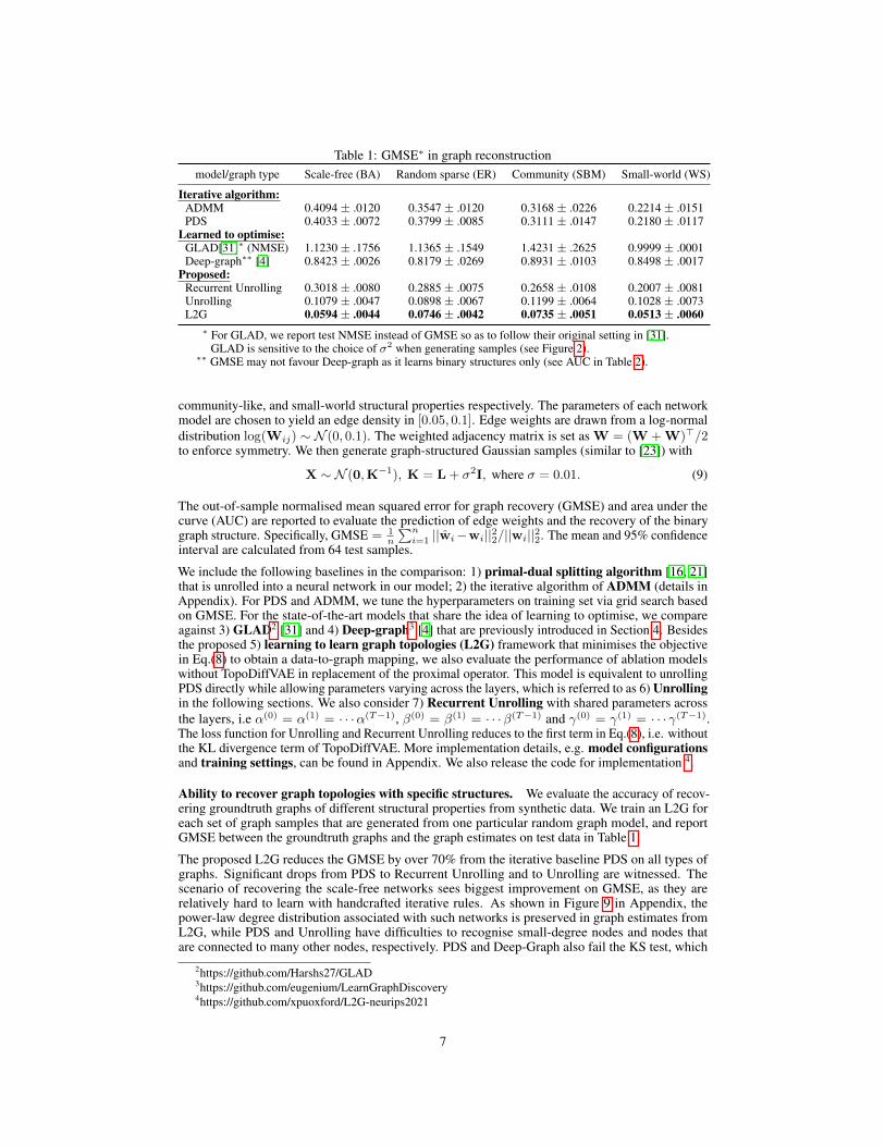
Table 1: GMSE⇤ in graph reconstructionmodel/graph type Scale-free (BA) Random sparse (ER) Community (SBM) Small-world (WS)

Iterative algorithm:

ADMM 0.4094 ± .0120 0.3547 ± .0120 0.3168 ± .0226 0.2214 ± .0151PDS 0.4033 ± .0072 0.3799 ± .0085 0.3111 ± .0147 0.2180 ± .0117

Learned to optimise:

GLAD[31]⇤ (NMSE) 1.1230 ± .1756 1.1365 ± .1549 1.4231 ± .2625 0.9999 ± .0001Deep-graph⇤⇤ [4] 0.8423 ± .0026 0.8179 ± .0269 0.8931 ± .0103 0.8498 ± .0017

Proposed:

Recurrent Unrolling 0.3018 ± .0080 0.2885 ± .0075 0.2658 ± .0108 0.2007 ± .0081Unrolling 0.1079 ± .0047 0.0898 ± .0067 0.1199 ± .0064 0.1028 ± .0073L2G 0.0594 ± .0044 0.0746 ± .0042 0.0735 ± .0051 0.0513 ± .0060

⇤ For GLAD, we report test NMSE instead of GMSE so as to follow their original setting in [31].GLAD is sensitive to the choice of �2 when generating samples (see Figure 2).

⇤⇤ GMSE may not favour Deep-graph as it learns binary structures only (see AUC in Table 2).

community-like, and small-world structural properties respectively. The parameters of each networkmodel are chosen to yield an edge density in [0.05, 0.1]. Edge weights are drawn from a log-normaldistribution log(Wij) ⇠ N (0, 0.1). The weighted adjacency matrix is set as W = (W +W)>/2to enforce symmetry. We then generate graph-structured Gaussian samples (similar to [23]) with

X ⇠ N (0,K�1), K = L+ �2I, where � = 0.01. (9)

The out-of-sample normalised mean squared error for graph recovery (GMSE) and area under thecurve (AUC) are reported to evaluate the prediction of edge weights and the recovery of the binarygraph structure. Specifically, GMSE = 1

n

Pni=1 ||wi�wi||22/||wi||22. The mean and 95% confidence

interval are calculated from 64 test samples.

We include the following baselines in the comparison: 1) primal-dual splitting algorithm [16, 21]that is unrolled into a neural network in our model; 2) the iterative algorithm of ADMM (details inAppendix). For PDS and ADMM, we tune the hyperparameters on training set via grid search basedon GMSE. For the state-of-the-art models that share the idea of learning to optimise, we compareagainst 3) GLAD

2 [31] and 4) Deep-graph3 [4] that are previously introduced in Section 4. Besides

the proposed 5) learning to learn graph topologies (L2G) framework that minimises the objectivein Eq.(8) to obtain a data-to-graph mapping, we also evaluate the performance of ablation modelswithout TopoDiffVAE in replacement of the proximal operator. This model is equivalent to unrollingPDS directly while allowing parameters varying across the layers, which is referred to as 6) Unrolling

in the following sections. We also consider 7) Recurrent Unrolling with shared parameters acrossthe layers, i.e ↵(0) = ↵(1) = · · ·↵(T�1), �(0) = �(1) = · · ·�(T�1) and �(0) = �(1) = · · · �(T�1).The loss function for Unrolling and Recurrent Unrolling reduces to the first term in Eq.(8), i.e. withoutthe KL divergence term of TopoDiffVAE. More implementation details, e.g. model configurations

and training settings, can be found in Appendix. We also release the code for implementation 4.

Ability to recover graph topologies with specific structures. We evaluate the accuracy of recov-ering groundtruth graphs of different structural properties from synthetic data. We train an L2G foreach set of graph samples that are generated from one particular random graph model, and reportGMSE between the groundtruth graphs and the graph estimates on test data in Table 1.

The proposed L2G reduces the GMSE by over 70% from the iterative baseline PDS on all types ofgraphs. Significant drops from PDS to Recurrent Unrolling and to Unrolling are witnessed. Thescenario of recovering the scale-free networks sees biggest improvement on GMSE, as they arerelatively hard to learn with handcrafted iterative rules. As shown in Figure 9 in Appendix, thepower-law degree distribution associated with such networks is preserved in graph estimates fromL2G, while PDS and Unrolling have difficulties to recognise small-degree nodes and nodes thatare connected to many other nodes, respectively. PDS and Deep-Graph also fail the KS test, which

2https://github.com/Harshs27/GLAD3https://github.com/eugenium/LearnGraphDiscovery4https://github.com/xpuoxford/L2G-neurips2021

7

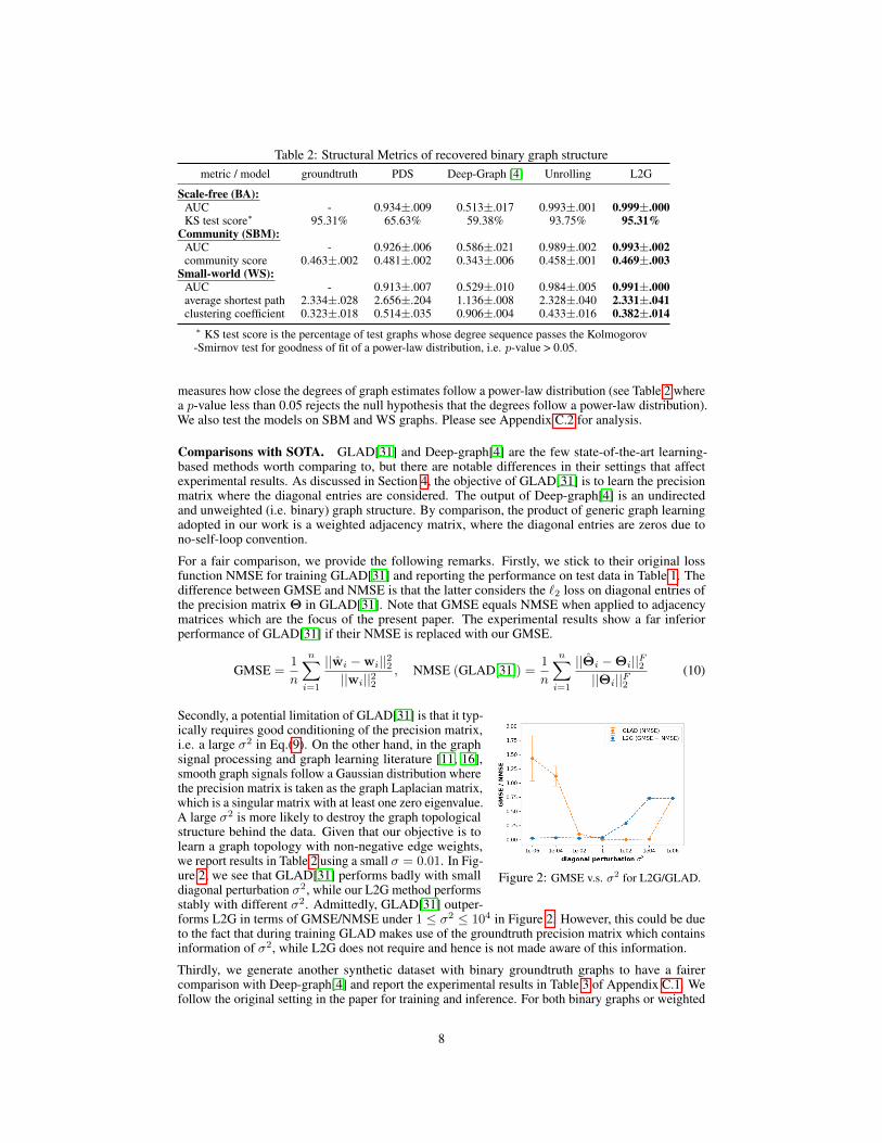
Table 2: Structural Metrics of recovered binary graph structuremetric / model groundtruth PDS Deep-Graph [4] Unrolling L2G

Scale-free (BA):

AUC - 0.934±.009 0.513±.017 0.993±.001 0.999±.000

KS test score⇤ 95.31% 65.63% 59.38% 93.75% 95.31%

Community (SBM):

AUC - 0.926±.006 0.586±.021 0.989±.002 0.993±.002

community score 0.463±.002 0.481±.002 0.343±.006 0.458±.001 0.469±.003

Small-world (WS):

AUC - 0.913±.007 0.529±.010 0.984±.005 0.991±.000

average shortest path 2.334±.028 2.656±.204 1.136±.008 2.328±.040 2.331±.041

clustering coefficient 0.323±.018 0.514±.035 0.906±.004 0.433±.016 0.382±.014

⇤ KS test score is the percentage of test graphs whose degree sequence passes the Kolmogorov-Smirnov test for goodness of fit of a power-law distribution, i.e. p-value > 0.05.

measures how close the degrees of graph estimates follow a power-law distribution (see Table 2 wherea p-value less than 0.05 rejects the null hypothesis that the degrees follow a power-law distribution).We also test the models on SBM and WS graphs. Please see Appendix C.2 for analysis.

Comparisons with SOTA. GLAD[31] and Deep-graph[4] are the few state-of-the-art learning-based methods worth comparing to, but there are notable differences in their settings that affectexperimental results. As discussed in Section 4, the objective of GLAD[31] is to learn the precisionmatrix where the diagonal entries are considered. The output of Deep-graph[4] is an undirectedand unweighted (i.e. binary) graph structure. By comparison, the product of generic graph learningadopted in our work is a weighted adjacency matrix, where the diagonal entries are zeros due tono-self-loop convention.

For a fair comparison, we provide the following remarks. Firstly, we stick to their original lossfunction NMSE for training GLAD[31] and reporting the performance on test data in Table 1. Thedifference between GMSE and NMSE is that the latter considers the `2 loss on diagonal entries ofthe precision matrix ⇥ in GLAD[31]. Note that GMSE equals NMSE when applied to adjacencymatrices which are the focus of the present paper. The experimental results show a far inferiorperformance of GLAD[31] if their NMSE is replaced with our GMSE.

GMSE =1

n

nX

i=1

||wi �wi||22||wi||22

, NMSE (GLAD[31]) =1

n

nX

i=1

||⇥i �⇥i||F2||⇥i||F2

(10)

Figure 2: GMSE v.s. �2 for L2G/GLAD.

Secondly, a potential limitation of GLAD[31] is that it typ-ically requires good conditioning of the precision matrix,i.e. a large �2 in Eq.(9). On the other hand, in the graphsignal processing and graph learning literature [11, 16],smooth graph signals follow a Gaussian distribution wherethe precision matrix is taken as the graph Laplacian matrix,which is a singular matrix with at least one zero eigenvalue.A large �2 is more likely to destroy the graph topologicalstructure behind the data. Given that our objective is tolearn a graph topology with non-negative edge weights,we report results in Table 2 using a small � = 0.01. In Fig-ure 2, we see that GLAD[31] performs badly with smalldiagonal perturbation �2, while our L2G method performsstably with different �2. Admittedly, GLAD[31] outper-forms L2G in terms of GMSE/NMSE under 1 �2 104 in Figure 2. However, this could be dueto the fact that during training GLAD makes use of the groundtruth precision matrix which containsinformation of �2, while L2G does not require and hence is not made aware of this information.

Thirdly, we generate another synthetic dataset with binary groundtruth graphs to have a fairercomparison with Deep-graph[4] and report the experimental results in Table 3 of Appendix C.1. Wefollow the original setting in the paper for training and inference. For both binary graphs or weighted

8

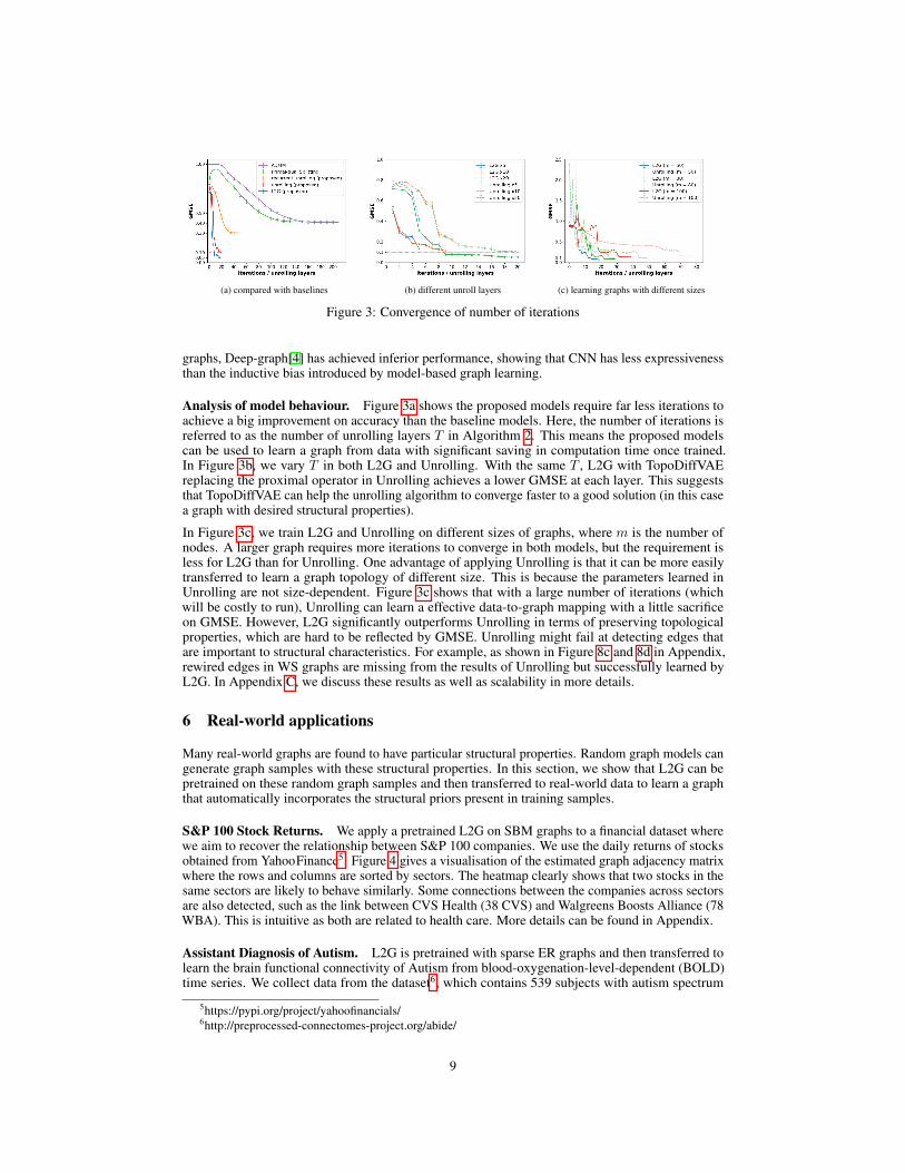
(a) compared with baselines (b) different unroll layers (c) learning graphs with different sizes

Figure 3: Convergence of number of iterations

graphs, Deep-graph[4] has achieved inferior performance, showing that CNN has less expressivenessthan the inductive bias introduced by model-based graph learning.

Analysis of model behaviour. Figure 3a shows the proposed models require far less iterations toachieve a big improvement on accuracy than the baseline models. Here, the number of iterations isreferred to as the number of unrolling layers T in Algorithm 2. This means the proposed modelscan be used to learn a graph from data with significant saving in computation time once trained.In Figure 3b, we vary T in both L2G and Unrolling. With the same T , L2G with TopoDiffVAEreplacing the proximal operator in Unrolling achieves a lower GMSE at each layer. This suggeststhat TopoDiffVAE can help the unrolling algorithm to converge faster to a good solution (in this casea graph with desired structural properties).

In Figure 3c, we train L2G and Unrolling on different sizes of graphs, where m is the number ofnodes. A larger graph requires more iterations to converge in both models, but the requirement isless for L2G than for Unrolling. One advantage of applying Unrolling is that it can be more easilytransferred to learn a graph topology of different size. This is because the parameters learned inUnrolling are not size-dependent. Figure 3c shows that with a large number of iterations (whichwill be costly to run), Unrolling can learn a effective data-to-graph mapping with a little sacrificeon GMSE. However, L2G significantly outperforms Unrolling in terms of preserving topologicalproperties, which are hard to be reflected by GMSE. Unrolling might fail at detecting edges thatare important to structural characteristics. For example, as shown in Figure 8c and 8d in Appendix,rewired edges in WS graphs are missing from the results of Unrolling but successfully learned byL2G. In Appendix C, we discuss these results as well as scalability in more details.

6 Real-world applications

Many real-world graphs are found to have particular structural properties. Random graph models cangenerate graph samples with these structural properties. In this section, we show that L2G can bepretrained on these random graph samples and then transferred to real-world data to learn a graphthat automatically incorporates the structural priors present in training samples.

S&P 100 Stock Returns. We apply a pretrained L2G on SBM graphs to a financial dataset wherewe aim to recover the relationship between S&P 100 companies. We use the daily returns of stocksobtained from YahooFinance5. Figure 4 gives a visualisation of the estimated graph adjacency matrixwhere the rows and columns are sorted by sectors. The heatmap clearly shows that two stocks in thesame sectors are likely to behave similarly. Some connections between the companies across sectorsare also detected, such as the link between CVS Health (38 CVS) and Walgreens Boosts Alliance (78WBA). This is intuitive as both are related to health care. More details can be found in Appendix.

Assistant Diagnosis of Autism. L2G is pretrained with sparse ER graphs and then transferred tolearn the brain functional connectivity of Autism from blood-oxygenation-level-dependent (BOLD)time series. We collect data from the dataset6, which contains 539 subjects with autism spectrum

5https://pypi.org/project/yahoofinancials/6http://preprocessed-connectomes-project.org/abide/

9

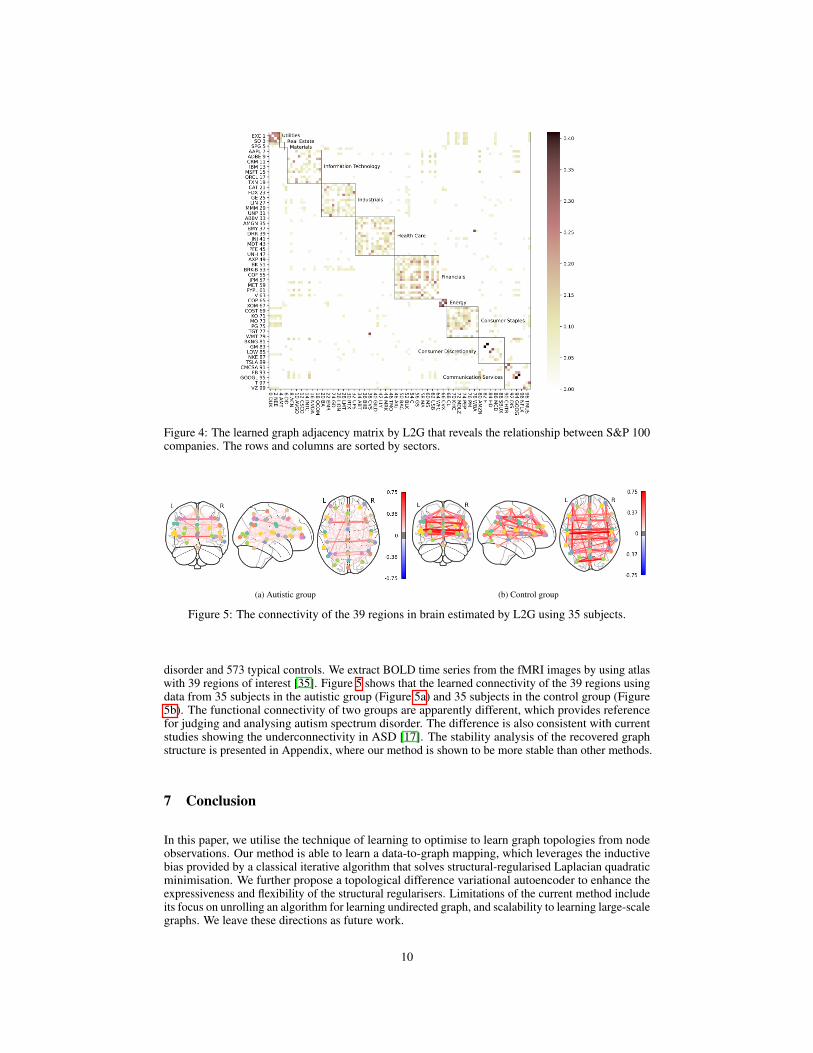
Figure 4: The learned graph adjacency matrix by L2G that reveals the relationship between S&P 100companies. The rows and columns are sorted by sectors.

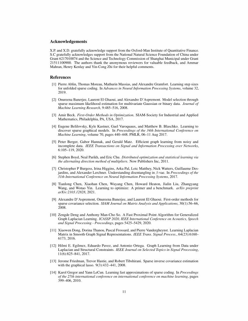
(a) Autistic group (b) Control group

Figure 5: The connectivity of the 39 regions in brain estimated by L2G using 35 subjects.

disorder and 573 typical controls. We extract BOLD time series from the fMRI images by using atlaswith 39 regions of interest [35]. Figure 5 shows that the learned connectivity of the 39 regions usingdata from 35 subjects in the autistic group (Figure 5a) and 35 subjects in the control group (Figure5b). The functional connectivity of two groups are apparently different, which provides referencefor judging and analysing autism spectrum disorder. The difference is also consistent with currentstudies showing the underconnectivity in ASD [17]. The stability analysis of the recovered graphstructure is presented in Appendix, where our method is shown to be more stable than other methods.

7 Conclusion

In this paper, we utilise the technique of learning to optimise to learn graph topologies from nodeobservations. Our method is able to learn a data-to-graph mapping, which leverages the inductivebias provided by a classical iterative algorithm that solves structural-regularised Laplacian quadraticminimisation. We further propose a topological difference variational autoencoder to enhance theexpressiveness and flexibility of the structural regularisers. Limitations of the current method includeits focus on unrolling an algorithm for learning undirected graph, and scalability to learning large-scalegraphs. We leave these directions as future work.

10

Acknowledgements

X.P. and X.D. gratefully acknowledge support from the Oxford-Man Institute of Quantitative Finance.S.C gratefully acknowledges support from the National Natural Science Foundation of China underGrant 6217010074 and the Science and Technology Commission of Shanghai Municipal under Grant21511100900. The authors thank the anonymous reviewers for valuable feedback, and AmmarMahran, Henry Kenlay and Yin-Cong Zhi for their helpful comments.

References

[1] Pierre Ablin, Thomas Moreau, Mathurin Massias, and Alexandre Gramfort. Learning step sizesfor unfolded sparse coding. In Advances in Neural Information Processing Systems, volume 32,2019.

[2] Onureena Banerjee, Laurent El Ghaoui, and Alexandre D’Aspremont. Model selection throughsparse maximum likelihood estimation for multivariate Gaussian or binary data. Journal of

Machine Learning Research, 9:485–516, 2008.

[3] Amir Beck. First-Order Methods in Optimization. SIAM-Society for Industrial and AppliedMathematics, Philadelphia, PA, USA, 2017.

[4] Eugene Belilovsky, Kyle Kastner, Gael Varoquaux, and Matthew B. Blaschko. Learning todiscover sparse graphical models. In Proceedings of the 34th International Conference on

Machine Learning, volume 70, pages 440–448. PMLR, 06–11 Aug 2017.

[5] Peter Berger, Gabor Hannak, and Gerald Matz. Efficient graph learning from noisy andincomplete data. IEEE Transactions on Signal and Information Processing over Networks,6:105–119, 2020.

[6] Stephen Boyd, Neal Parikh, and Eric Chu. Distributed optimization and statistical learning via

the alternating direction method of multipliers. Now Publishers Inc, 2011.

[7] Christopher P Burgess, Irina Higgins, Arka Pal, Loic Matthey, Nick Watters, Guillaume Des-jardins, and Alexander Lerchner. Understanding disentangling in �-vae. In Proceedings of the

31th International Conference on Neural Information Processing Systems, 2017.

[8] Tianlong Chen, Xiaohan Chen, Wuyang Chen, Howard Heaton, Jialin Liu, ZhangyangWang, and Wotao Yin. Learning to optimize: A primer and a benchmark. arXiv preprint

arXiv:2103.12828, 2021.

[9] Alexandre D’Aspremont, Onureena Banerjee, and Laurent El Ghaoui. First-order methods forsparse covariance selection. SIAM Journal on Matrix Analysis and Applications, 30(1):56–66,2008.

[10] Zengde Deng and Anthony Man-Cho So. A Fast Proximal Point Algorithm for GeneralizedGraph Laplacian Learning. ICASSP 2020, IEEE International Conference on Acoustics, Speech

and Signal Processing - Proceedings, pages 5425–5429, 2020.

[11] Xiaowen Dong, Dorina Thanou, Pascal Frossard, and Pierre Vandergheynst. Learning LaplacianMatrix in Smooth Graph Signal Representations. IEEE Trans. Signal Process., 64(23):6160–6173, 2016.

[12] Hilmi E. Egilmez, Eduardo Pavez, and Antonio Ortega. Graph Learning from Data underLaplacian and Structural Constraints. IEEE Journal on Selected Topics in Signal Processing,11(6):825–841, 2017.

[13] Jerome Friedman, Trevor Hastie, and Robert Tibshirani. Sparse inverse covariance estimationwith the graphical lasso. 9(3):432–441, 2008.

[14] Karol Gregor and Yann LeCun. Learning fast approximations of sparse coding. In Proceedings

of the 27th international conference on international conference on machine learning, pages399–406, 2010.

11

[15] Dominique Guillot, Bala Rajaratnam, Benjamin T Rolfs, Arian Maleki, and Ian Wong. Iterativethresholding algorithm for sparse inverse covariance estimation. In Proceedings of the 25th

International Conference on Neural Information Processing Systems, 2012.

[16] Vassilis Kalofolias. How to learn a graph from smooth signals. Proc. 19th Int. Conf. Artif. Intell.

Stat. AISTATS 2016, jan 2016.

[17] Rajesh K. Kana, Lauren E. Libero, and Marie S. Moore. Disrupted cortical connectivity theoryas an explanatory model for autism spectrum disorders. Physics of Life Reviews, 8(4):410–437,2011.

[18] Diederik P. Kingma and Jimmy Ba. Adam: A method for stochastic optimization. In ICLR

(Poster), 2015.

[19] Diederik P. Kingma and Max Welling. Auto-encoding variational bayes. In Proceedings of the

2nd International Conference on Learning Representations (ICLR), 2014.

[20] Thomas N Kipf and Max Welling. Semi-supervised classification with graph convolutionalnetworks. In International Conference on Learning Representations, 2017.

[21] Nikos Komodakis and Jean-Christophe Pesquet. Playing with duality: An overview of recentprimal? dual approaches for solving large-scale optimization problems. IEEE Signal Processing

Magazine, 32(6):31–54, 2015.

[22] Sandeep Kumar, Jiaxi Ying, Jose Vinicius de Miranda Cardoso, and Daniel Palomar. Structuredgraph learning via laplacian spectral constraints. In H. Wallach, H. Larochelle, A. Beygelzimer,F. d'Alché-Buc, E. Fox, and R. Garnett, editors, Advances in Neural Information Processing

Systems, volume 32. Curran Associates, Inc., 2019.

[23] Brenden M Lake and Joshua B Tenenbaum. Discovering Structure by Learning Sparse Graphs.Proceedings of the 32nd Annual Conference of the Cognitive Science Society, 2010.

[24] Steffen L Lauritzen. Graphical models. Clarendon Press, 1996.

[25] Zhaosong Lu. Adaptive first-order methods for general sparse inverse covariance selection.SIAM Journal on Matrix Analysis and Applications, 31(4):2000–2016, 2009.

[26] Vishal Monga, Yuelong Li, and Yonina C Eldar. Algorithm unrolling: Interpretable, efficientdeep learning for signal and image processing. IEEE Signal Processing Magazine, 38(2):18–44,2021.

[27] Thomas Moreau and Joan Bruna. Understanding the learned iterative soft thresholding algo-rithm with matrix factorization. In Proceedings of the International Conference on Learning

Representations (ICLR), 2017.

[28] Antonio Ortega, Pascal Frossard, Jelena Kovacevic, José MF Moura, and Pierre Vandergheynst.Graph signal processing: Overview, challenges, and applications. Proceedings of the IEEE,106(5):808–828, 2018.

[29] JH Rick Chang, Chun-Liang Li, Barnabas Poczos, BVK Vijaya Kumar, and Aswin C Sankara-narayanan. One network to solve them all–solving linear inverse problems using deep projectionmodels. In Proceedings of the IEEE International Conference on Computer Vision, pages5888–5897, 2017.

[30] Aliaksei Sandryhaila and José MF Moura. Discrete signal processing on graphs. IEEE

transactions on signal processing, 61(7):1644–1656, 2013.

[31] Harsh Shrivastava, Xinshi Chen, Binghong Chen, Guanghui Lan, Srinivas Aluru, Han Liu, andLe Song. Glad: Learning sparse graph recovery. In International Conference on Learning

Representations, 2020.

[32] David Shuman, Sunil Narang, Pascal Frossard, Antonio Ortega, and Pierre Vandergheynst. Theemerging field of signal processing on graphs: Extending high-dimensional data analysis tonetworks and other irregular domains. IEEE Signal Processing Magazine, 3(30):83–98, 2013.

12

[33] Martin Slawski and Matthias Hein. Estimation of positive definite M-matrices and structurelearning for attractive Gaussian Markov random fields. Linear Algebra and Its Applications,473:145–179, 5 2015.

[34] Pablo Sprechmann, Roee Litman, Tal Ben Yakar, Alexander M Bronstein, and GuillermoSapiro. Supervised sparse analysis and synthesis operators. In Advances in Neural Information

Processing Systems, volume 26, pages 908–916, 2013.

[35] Gael Varoquaux, Alexandre Gramfort, Fabian Pedregosa, Vincent Michel, and Bertrand Thirion.Multi-subject dictionary learning to segment an atlas of brain spontaneous activity. In GáborSzékely and Horst K. Hahn, editors, Information Processing in Medical Imaging, pages 562–573,Berlin, Heidelberg, 2011. Springer Berlin Heidelberg.

[36] Duncan J Watts and Steven H Strogatz. Collective dynamics of ‘small-world’networks. nature,393(6684):440–442, 1998.

[37] Kai Zhang, Wangmeng Zuo, Shuhang Gu, and Lei Zhang. Learning deep cnn denoiser priorfor image restoration. In Proceedings of the IEEE conference on computer vision and pattern

recognition, pages 3929–3938, 2017.

13

Checklist

1. For all authors...(a) Do the main claims made in the abstract and introduction accurately reflect the paper’s

contributions and scope? [Yes] See Abstract and Section 1.(b) Did you describe the limitations of your work? [Yes] See Section 7.(c) Did you discuss any potential negative societal impacts of your work? [No](d) Have you read the ethics review guidelines and ensured that your paper conforms to

them? [Yes]2. If you are including theoretical results...

(a) Did you state the full set of assumptions of all theoretical results? [Yes] See Section 2.(b) Did you include complete proofs of all theoretical results? [No]

3. If you ran experiments...(a) Did you include the code, data, and instructions needed to reproduce the main experi-

mental results (either in the supplemental material or as a URL)? [Yes] See Section 5.(b) Did you specify all the training details (e.g., data splits, hyperparameters, how they

were chosen)? [Yes] See Section 5.(c) Did you report error bars (e.g., with respect to the random seed after running experi-

ments multiple times)? [Yes] See Section 5 we report confidence intervals.(d) Did you include the total amount of compute and the type of resources used (e.g., type

of GPUs, internal cluster, or cloud provider)? [Yes] See Section 5.4. If you are using existing assets (e.g., code, data, models) or curating/releasing new assets...

(a) If your work uses existing assets, did you cite the creators? [Yes] See Section 5.(b) Did you mention the license of the assets? [Yes] See Section 5.(c) Did you include any new assets either in the supplemental material or as a URL? [Yes](d) Did you discuss whether and how consent was obtained from people whose data you’re

using/curating? [No](e) Did you discuss whether the data you are using/curating contains personally identifiable

information or offensive content? [No]5. If you used crowdsourcing or conducted research with human subjects...

(a) Did you include the full text of instructions given to participants and screenshots, ifapplicable? [N/A]

(b) Did you describe any potential participant risks, with links to Institutional ReviewBoard (IRB) approvals, if applicable? [N/A]

(c) Did you include the estimated hourly wage paid to participants and the total amountspent on participant compensation? [N/A]

14