Learning Sequence Motif Models Using Gibbs Sampling
32
Learning Sequence Motif Models Using Gibbs Sampling BMI/CS 776 www.biostat.wisc.edu/bmi776/ Spring 2012 Colin Dewey [email protected]
Transcript of Learning Sequence Motif Models Using Gibbs Sampling
Learning Sequence Motif Models Using Gibbs Sampling
BMI/CS 776 www.biostat.wisc.edu/bmi776/
Spring 2012 Colin Dewey
Goals for Lecture
the key concepts to understand are the following • Markov Chain Monte Carlo (MCMC) and Gibbs sampling • Gibbs sampling applied to the motif-finding task • parameter tying • incorporating prior knowledge using Dirichlets and
Dirichlet mixtures
Gibbs Sampling: An Alternative to EM
• EM can get trapped in local minima • one approach to alleviate this limitation: try different
(perhaps random) initial parameters • Gibbs sampling exploits randomized search to a
much greater degree • can view it as a stochastic analog of EM for this task • in theory, Gibbs sampling is less susceptible to local
minima than EM • [Lawrence et al., Science 1993]
Gibbs Sampling Approach
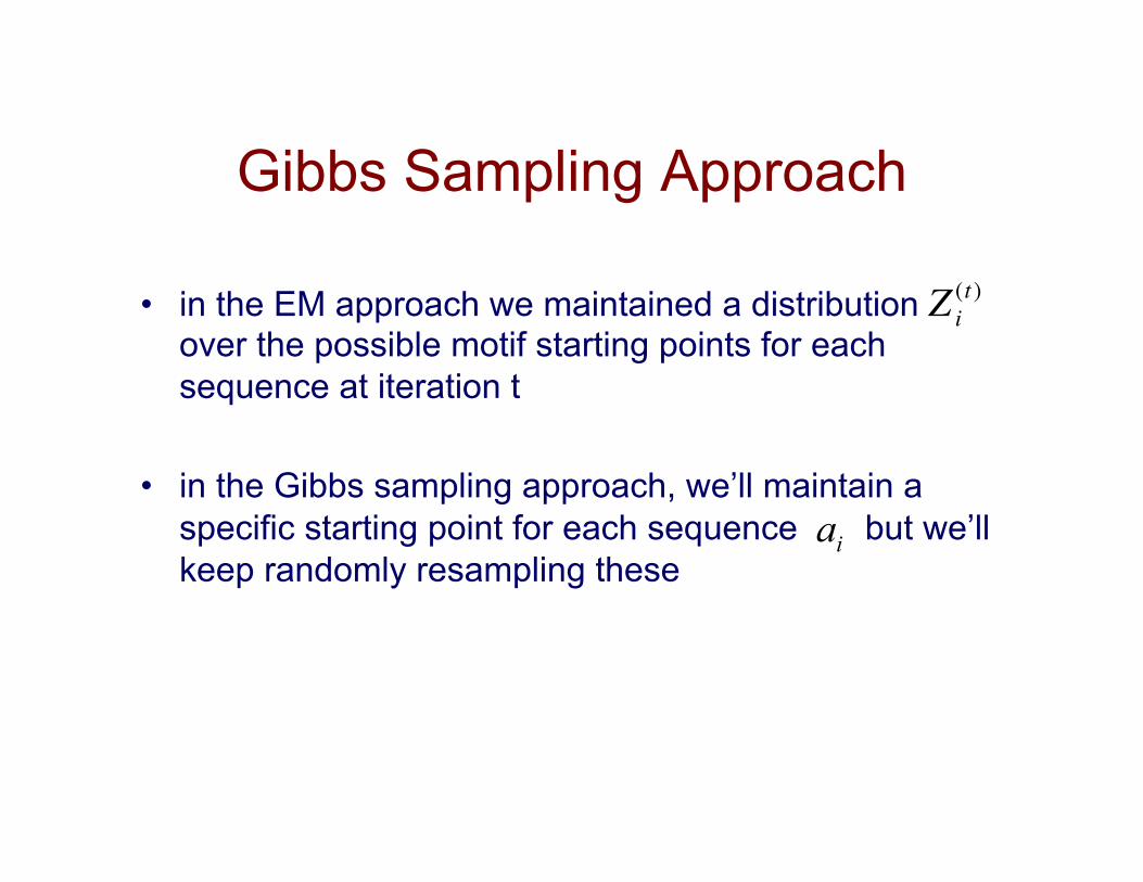
• in the EM approach we maintained a distribution over the possible motif starting points for each sequence at iteration t
• in the Gibbs sampling approach, we’ll maintain a specific starting point for each sequence but we’ll keep randomly resampling these
Z (t )i
ia
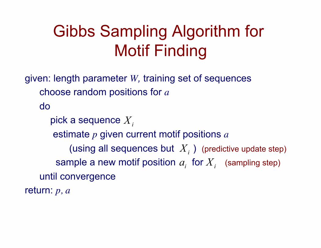
Gibbs Sampling Algorithm for Motif Finding
given: length parameter W, training set of sequences choose random positions for a do pick a sequence estimate p given current motif positions a (using all sequences but ) (predictive update step)
sample a new motif position for (sampling step)
until convergence return: p, a
iX
iXiXia
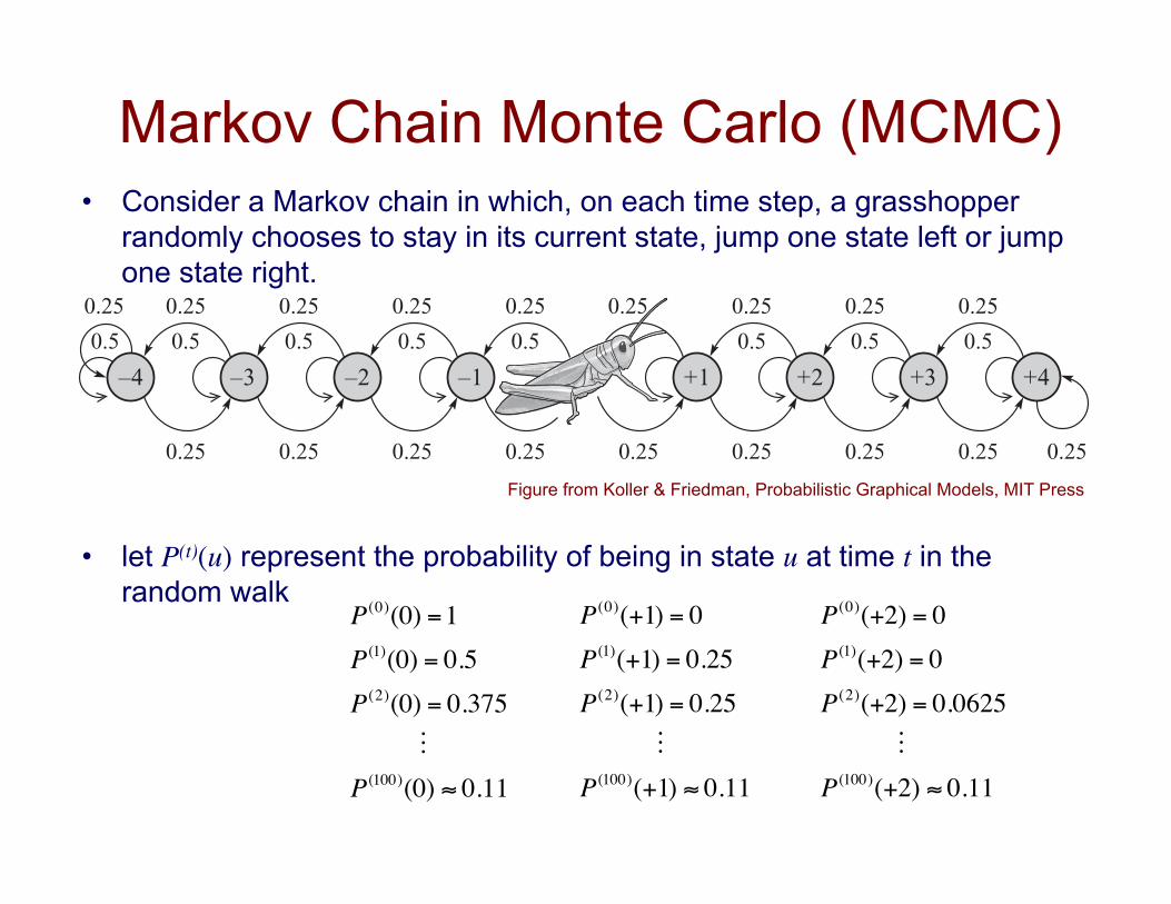
Markov Chain Monte Carlo (MCMC) • Consider a Markov chain in which, on each time step, a grasshopper
randomly chooses to stay in its current state, jump one state left or jump one state right.
0.250.25
0.50.5
0.25
0.5
0.25
0.5
0.25
0.5
0.25 0.25
0.5
0.25
0.5
0.25
0.25 0.25 0.25 0.25 0.25 0.25 0.25 0.25 0.25
0.5
–3–4 –2 –1 +1 +2 +3 +4
• let P(t)(u) represent the probability of being in state u at time t in the random walk
€
P(0)(0) =1P(1)(0) = 0.5P(2)(0) = 0.375 P(100)(0) ≈ 0.11
€
P(0)(+1) = 0P(1)(+1) = 0.25P(2)(+1) = 0.25 P(100)(+1) ≈ 0.11
€
P(0)(+2) = 0P(1)(+2) = 0P(2)(+2) = 0.0625 P(100)(+2) ≈ 0.11
Figure from Koller & Friedman, Probabilistic Graphical Models, MIT Press
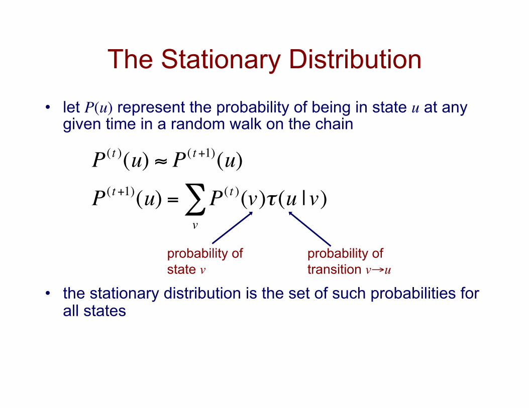
The Stationary Distribution • let P(u) represent the probability of being in state u at any
given time in a random walk on the chain
• the stationary distribution is the set of such probabilities for all states €
P(t )(u) ≈ P( t+1)(u)
P(t+1)(u) = P( t )(v)τ (u | v)v∑
probability of state v
probability of transition v→u
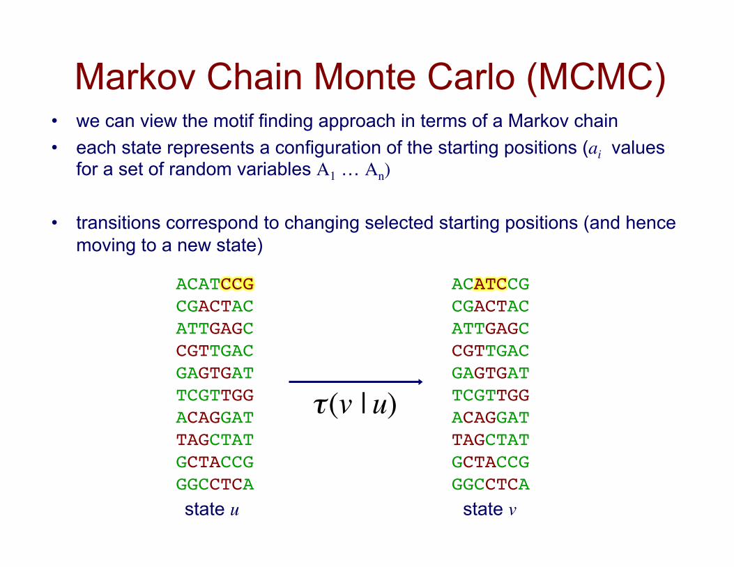
Markov Chain Monte Carlo (MCMC) • we can view the motif finding approach in terms of a Markov chain • each state represents a configuration of the starting positions (ai values
for a set of random variables A1 … An)
• transitions correspond to changing selected starting positions (and hence moving to a new state)
ACATCCG!CGACTAC!ATTGAGC!CGTTGAC!GAGTGAT!TCGTTGG!ACAGGAT!TAGCTAT!GCTACCG!GGCCTCA!
ACATCCG!CGACTAC!ATTGAGC!CGTTGAC!GAGTGAT!TCGTTGG!ACAGGAT!TAGCTAT!GCTACCG!GGCCTCA!
state u state v €
τ(v | u)

Markov Chain Monte Carlo • for the motif-finding task, the number of states is enormous • key idea: construct Markov chain with stationary
distribution equal to distribution of interest; use sampling to find most probable states
• detailed balance:
€
P(u)τ(v | u) = P(v)τ (u | v)
€
1NlimN→∞ count(u) = P(u)
probability of state u
probability of transition u→v
• when detailed balance holds:
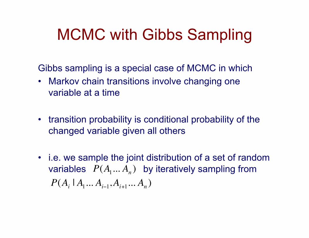
MCMC with Gibbs Sampling
Gibbs sampling is a special case of MCMC in which • Markov chain transitions involve changing one
variable at a time
• transition probability is conditional probability of the changed variable given all others
• i.e. we sample the joint distribution of a set of random variables by iteratively sampling from
€
P(Ai | A1... Ai−1,Ai+1... An )
€
P(A1... An )
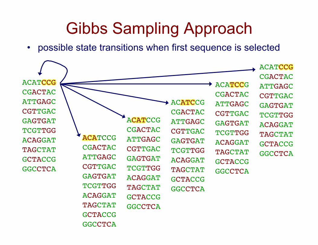
Gibbs Sampling Approach
ACATCCG!CGACTAC!ATTGAGC!CGTTGAC!GAGTGAT!TCGTTGG!ACAGGAT!TAGCTAT!GCTACCG!GGCCTCA!
ACATCCG!CGACTAC!ATTGAGC!CGTTGAC!GAGTGAT!TCGTTGG!ACAGGAT!TAGCTAT!GCTACCG!GGCCTCA!
• possible state transitions when first sequence is selected
ACATCCG!CGACTAC!ATTGAGC!CGTTGAC!GAGTGAT!TCGTTGG!ACAGGAT!TAGCTAT!GCTACCG!GGCCTCA!
ACATCCG!CGACTAC!ATTGAGC!CGTTGAC!GAGTGAT!TCGTTGG!ACAGGAT!TAGCTAT!GCTACCG!GGCCTCA!
ACATCCG!CGACTAC!ATTGAGC!CGTTGAC!GAGTGAT!TCGTTGG!ACAGGAT!TAGCTAT!GCTACCG!GGCCTCA!
ACATCCG!CGACTAC!ATTGAGC!CGTTGAC!GAGTGAT!TCGTTGG!ACAGGAT!TAGCTAT!GCTACCG!GGCCTCA!
Gibbs Sampling Approach
• How do we get the transition probabilities when we don’t know what the motif looks like?
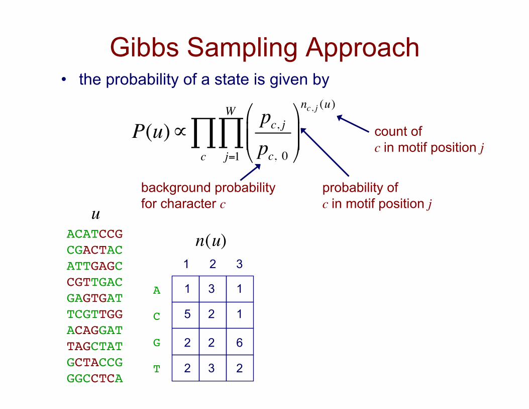
Gibbs Sampling Approach • the probability of a state is given by
P(u)∝pc, jpc, 0
"
#$$
%
&''
nc, j (u)
j=1
W
∏c∏
ACATCCG!CGACTAC!ATTGAGC!CGTTGAC!GAGTGAT!TCGTTGG!ACAGGAT!TAGCTAT!GCTACCG!GGCCTCA!
A!
C!
G!
T!
1 2 3
1
1
6
2
1
5
2
2 3
2
2
3
count of c in motif position j
probability of c in motif position j
background probability for character c
€
n(u)
€
u
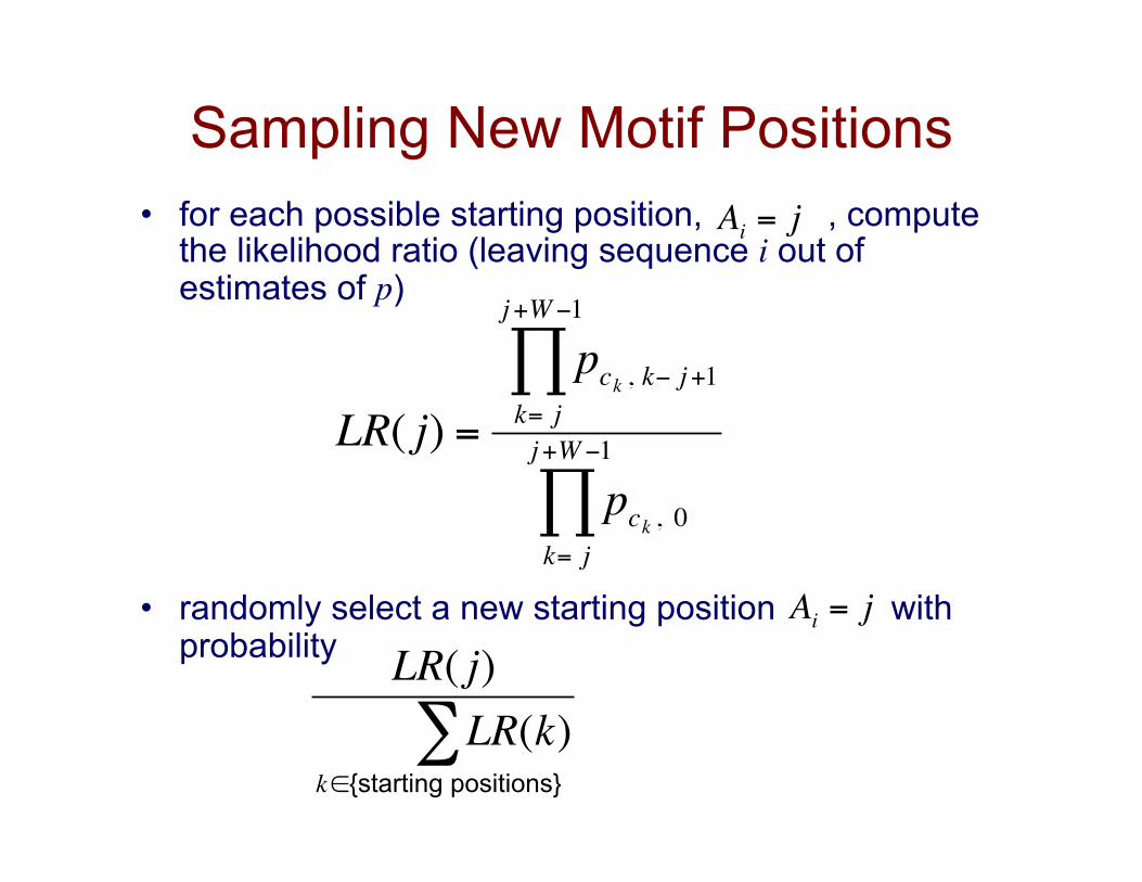
Sampling New Motif Positions • for each possible starting position, , compute
the likelihood ratio (leaving sequence i out of estimates of p)
• randomly select a new starting position with probability
€
LR( j) =
pck , k− j+1k= j
j+W −1
∏
pck , 0k= j
j+W −1
∏
€
Ai = j
€
Ai = j
€
LR( j)LR(k)
k∈{starting positions}
∑
The Phase Shift Problem
• Gibbs sampler can get stuck in a local maximum that corresponds to the correct solution shifted by a few bases
• solution: add a special step to shift the a values by the same amount for all sequences. Try different shift amounts and pick one in proportion to its probability score
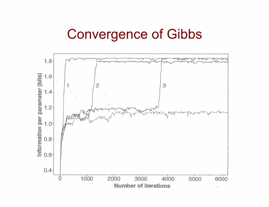
Convergence of Gibbs
Using Background Knowledge to Bias the Parameters
let’s consider two ways in which background knowledge can be exploited in the motif finding process
1. accounting for palindromes that are common in
DNA binding sites 2. using Dirichlet mixture priors to account for
biochemical similarity of amino acids
Using Background Knowledge to Bias the Parameters
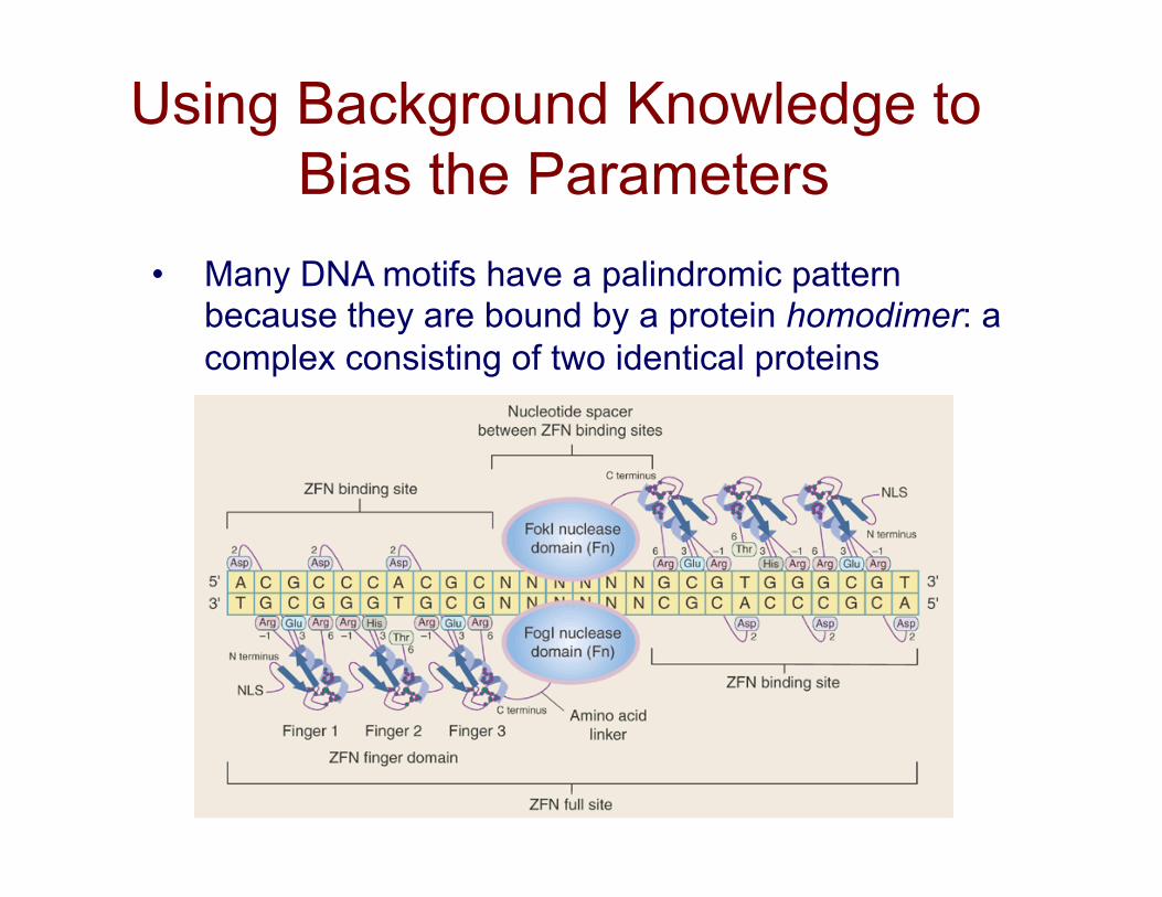
• Many DNA motifs have a palindromic pattern because they are bound by a protein homodimer: a complex consisting of two identical proteins
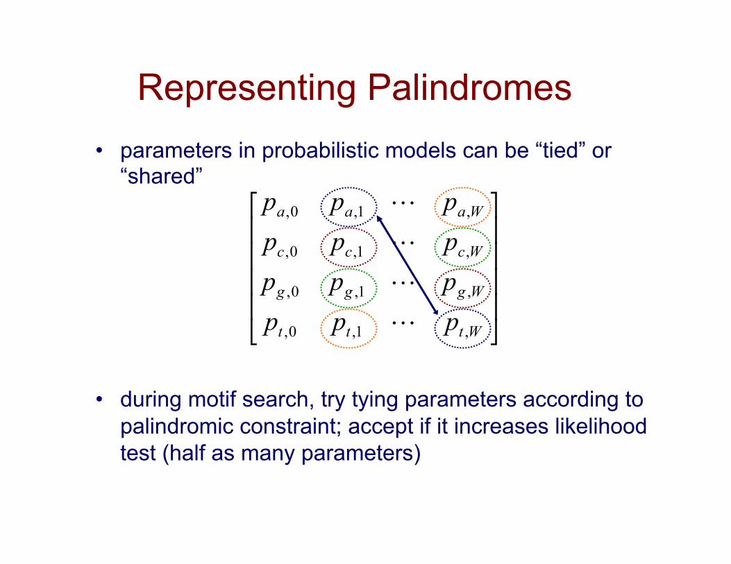
Representing Palindromes • parameters in probabilistic models can be “tied” or
“shared”
• during motif search, try tying parameters according to palindromic constraint; accept if it increases likelihood test (half as many parameters)
!!!!
"
#
$$$$
%
&
Wttt
Wggg
Wccc
Waaa
pppppppppppp
,1,0,
,1,0,
,1,0,
,1,0,
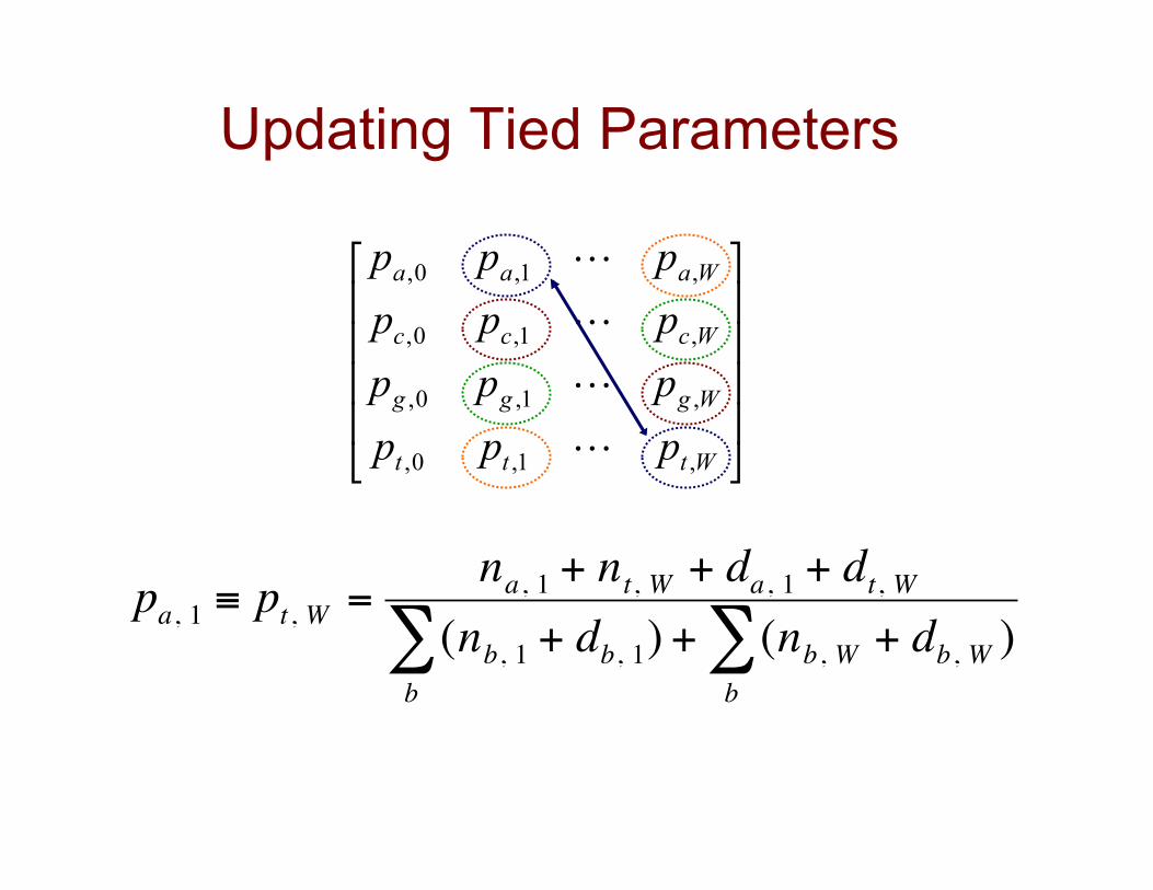
Updating Tied Parameters
!!!!
"
#
$$$$
%
&
Wttt
Wggg
Wccc
Waaa
pppppppppppp
,1,0,
,1,0,
,1,0,
,1,0,
€
pa, 1 ≡ pt , W =na, 1 + nt, W + da, 1 + dt, W
(nb, 1 + db, 1) + (nb, W + db, W )b∑
b∑
Using Dirichlet Mixture Priors
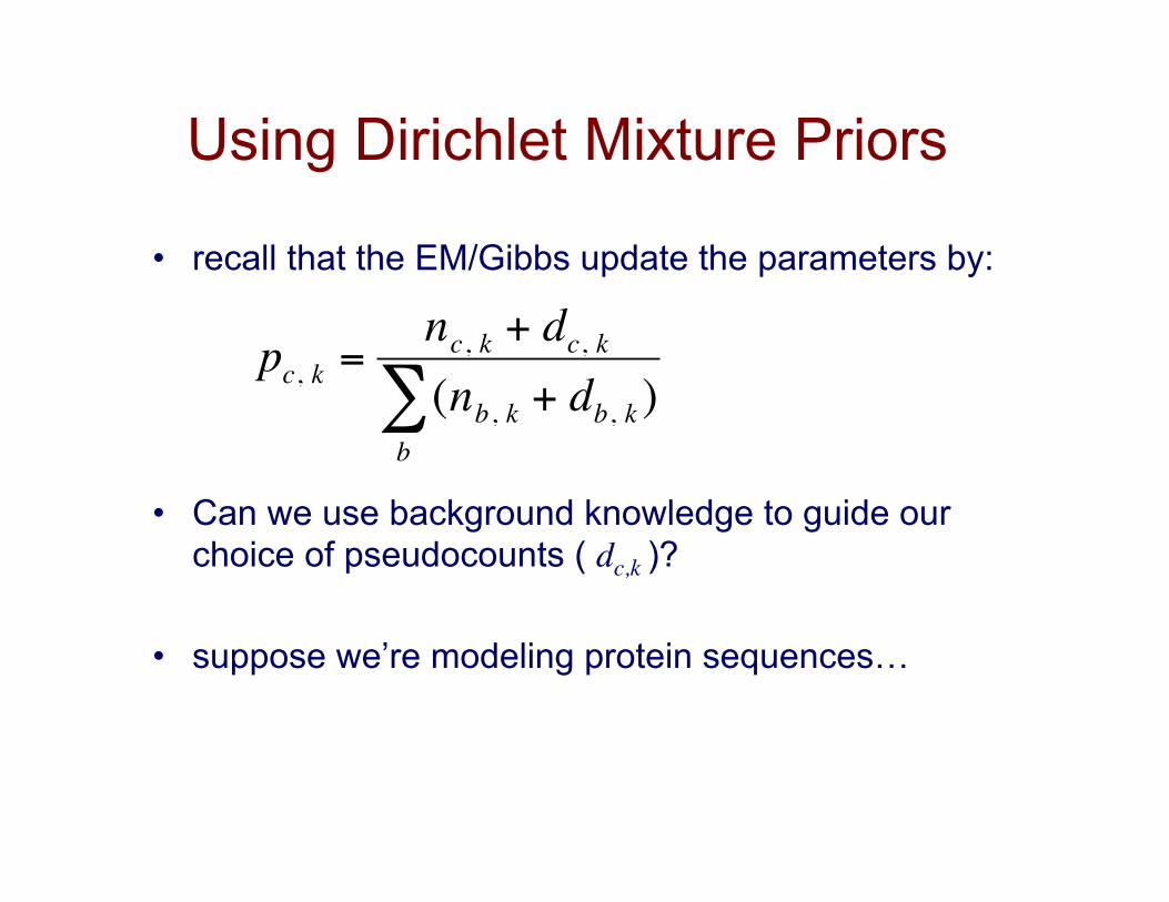
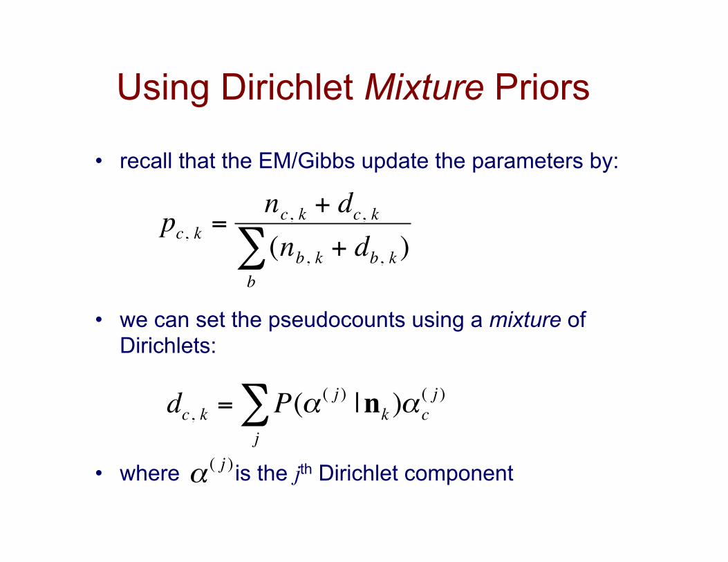
• recall that the EM/Gibbs update the parameters by:
• Can we use background knowledge to guide our choice of pseudocounts ( dc,k )?
• suppose we’re modeling protein sequences…
€
pc, k =nc, k + dc, k(nb, k + db, k )
b∑
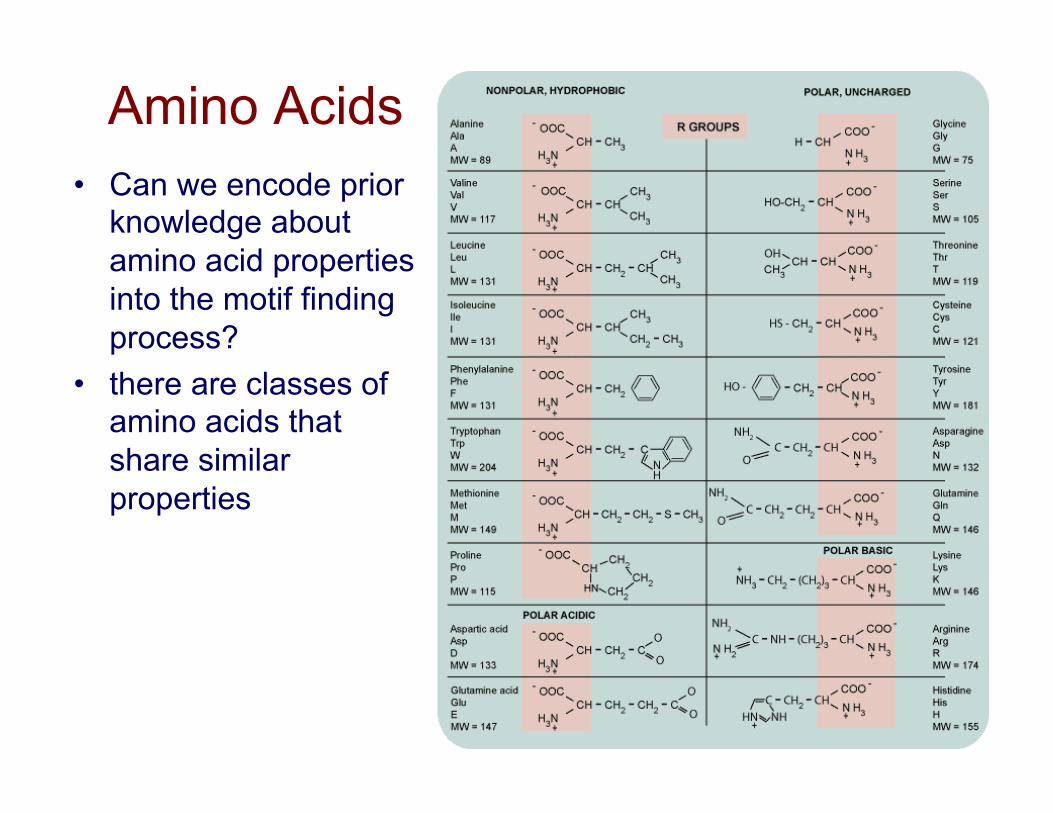
Amino Acids • Can we encode prior
knowledge about amino acid properties into the motif finding process?
• there are classes of amino acids that share similar properties
Using Dirichlet Mixture Priors
• since we’re estimating multinomial distributions (frequencies of amino acids at each motif position), a natural way to encode prior knowledge is using Dirichlet distributions
• let’s consider • the Beta distribution • the Dirichlet distribution • mixtures of Dirichlets
The Beta Distribution
11 )1()()()()( −− −
ΓΓ
+Γ= th
th
thP αα θθαααα
θ
hα
tα
0 1
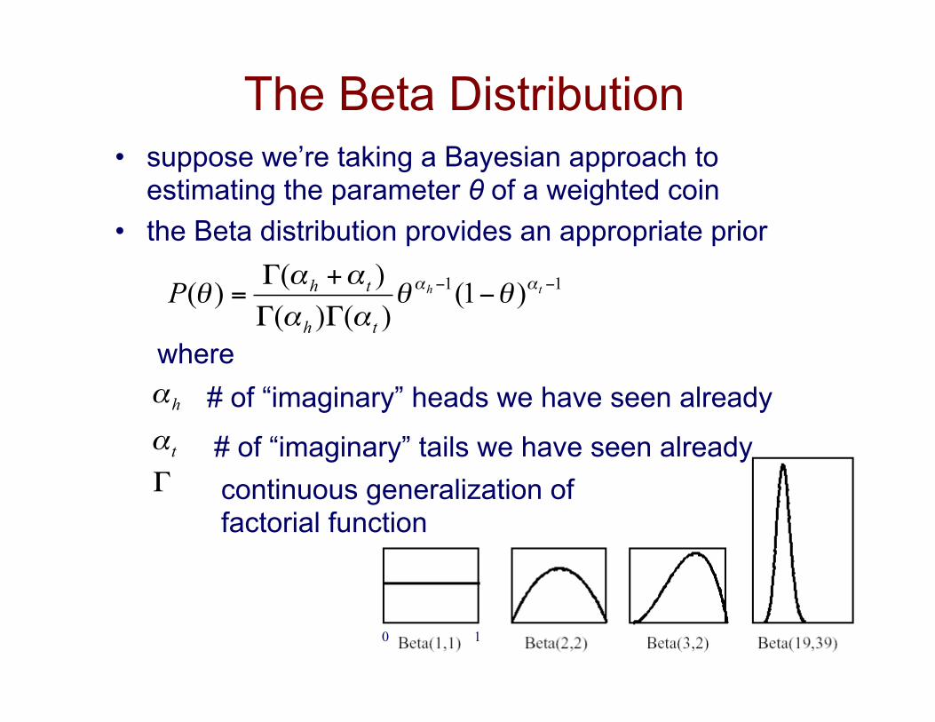
• suppose we’re taking a Bayesian approach to estimating the parameter θ of a weighted coin
• the Beta distribution provides an appropriate prior
where
Γ
# of “imaginary” heads we have seen already
# of “imaginary” tails we have seen already continuous generalization of factorial function
The Beta Distribution
€
P(θ |D) =Γ(α + Dh + Dt )
Γ(αh + Dh )Γ(α t + Dt )θαh +Dh−1(1−θ)α t +Dt −1
= Beta(αh + Dh ,α t + Dt )
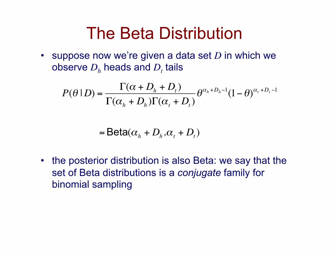
• suppose now we’re given a data set D in which we observe Dh heads and Dt tails
• the posterior distribution is also Beta: we say that the set of Beta distributions is a conjugate family for binomial sampling
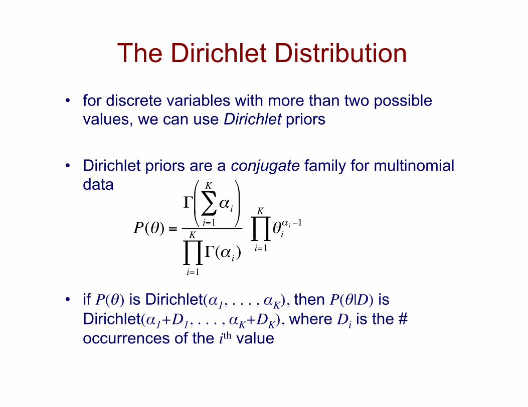
The Dirichlet Distribution • for discrete variables with more than two possible
values, we can use Dirichlet priors
• Dirichlet priors are a conjugate family for multinomial data
• if P(θ) is Dirichlet(α1, . . . , αK), then P(θ|D) is Dirichlet(α1+D1, . . . , αK+DK), where Di is the # occurrences of the ith value
€
P(θ) =
Γ α ii=1
K
∑&
' (
)
* +
Γ(α i)i=1
K
∏ θi
α i −1
i=1
K
∏
Dirichlet Distributions
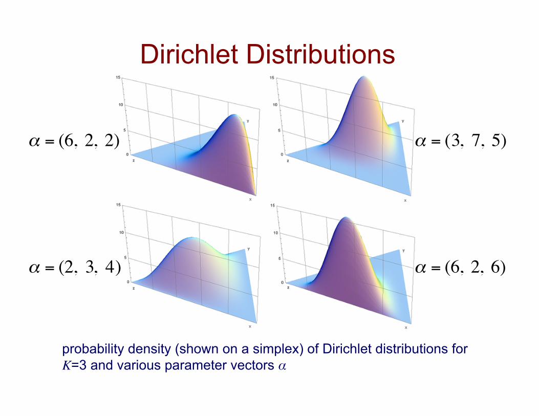
probability density (shown on a simplex) of Dirichlet distributions for K=3 and various parameter vectors α
€
α = (6, 2, 2)
€
α = (3, 7, 5)
€
α = (6, 2, 6)
€
α = (2, 3, 4)
Mixture of Dirichlets
• we’d like to have Dirichlet distributions characterizing amino acids that tend to be used in certain “roles”
• Brown et al. [ISMB ‘95] induced a set of Dirichlets from “trusted” protein alignments – “large, charged and polar” – “polar and mostly negatively charged” – “hydrophobic, uncharged, nonpolar” – etc.
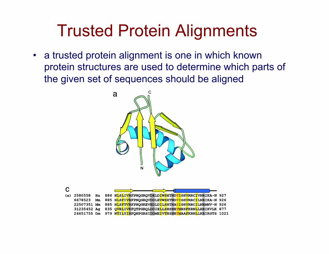
Trusted Protein Alignments • a trusted protein alignment is one in which known
protein structures are used to determine which parts of the given set of sequences should be aligned
Using Dirichlet Mixture Priors
• recall that the EM/Gibbs update the parameters by:
• we can set the pseudocounts using a mixture of Dirichlets:
• where is the jth Dirichlet component
€
pc, k =nc, k + dc, k(nb, k + db, k )
b∑
€
dc, k = P(α ( j )
j∑ |nk )αc
( j )
€
α ( j )
Using Dirichlet Mixture Priors
€
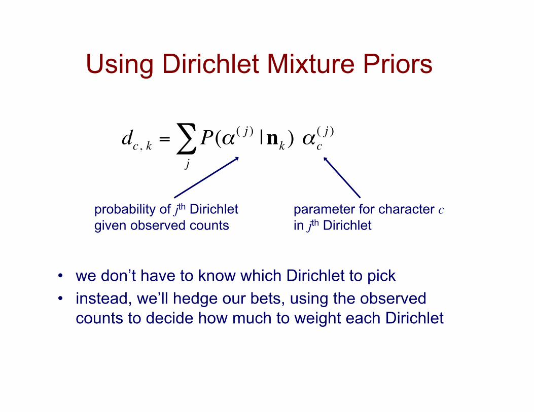
dc, k = P(α ( j )
j∑ |nk ) α c
( j )
probability of jth Dirichlet given observed counts
parameter for character c in jth Dirichlet
• we don’t have to know which Dirichlet to pick • instead, we’ll hedge our bets, using the observed
counts to decide how much to weight each Dirichlet
Motif Finding: EM and Gibbs • these methods compute local, multiple alignments • both methods try to optimize the likelihood of the sequences • EM converges to a local maximum • Gibbs will “converge” to a global maximum, in the limit; in a reasonable
amount of time, probably not • can take advantage of background knowledge by
– tying parameters – Dirichlet priors
• there are many other methods for motif finding • in practice, motif finders often fail
– motif “signal” may be weak – large search space, many local minima