Learning Quadrotor Dynamics Using Neural Network for Flight Control

Somil Bansal∗ Anayo K. Akametalu∗ Frank J. Jiang Forrest Laine Claire J. Tomlin

Abstract— Traditional learning approaches proposed for con-trolling quadrotors or helicopters have focused on improvingperformance for specific trajectories by iteratively improvingupon a nominal controller, for example learning from demon-strations, iterative learning, and reinforcement learning. Inthese schemes, however, it is not clear how the informationgathered from the training trajectories can be used to synthesizecontrollers for more general trajectories. Recently, the efficacyof deep learning in inferring helicopter dynamics has beenshown. Motivated by the generalization capability of deeplearning, this paper investigates whether a neural networkbased dynamics model can be employed to synthesize control fortrajectories different than those used for training. To test this,we learn a quadrotor dynamics model using only translationaland only rotational training trajectories, each of which canbe controlled independently, and then use it to simultaneouslycontrol the yaw and position of a quadrotor, which is non-trivialbecause of nonlinear couplings between the two motions. Wevalidate our approach in experiments on a quadrotor testbed.

I. INTRODUCTION

System identification, the mathematical modeling of asystem’s dynamics, is one of the most basic and importantcomponents of control. Constructing an appropriate modelis often the first step in designing a controller. Modelingaccuracy, therefore, directly impacts controller success andperformance, as inaccuracies in the model appear to thecontroller as external disturbances.

Quadrotors have recently emerged as a popular platformfor unmanned aerial vehicle (UAV) research, due to thesimplicity of their construction and maintenance. Quadrotorscan be highly maneuverable, and have the potential to hover,take off, fly and land in small areas due to a vertical takeoff and landing (VTOL) capability [8]. A quadrotor has fourrotors located at the four corners of a cross frame, and iscontrolled by changing the speed of rotation of the four rotors[4], [21]. However, the system is under-actuated, nonlinearand difficult to control on aggressive trajectories. Most ofthe work in this area focuses on designing controllers thatare derived from a linearization of the model around hoverconditions and are stable only under reasonably small rolland pitch angles. While advanced control methods such asfeedback linearization [20], adaptive control [13], sliding-mode control [22], H∞ robust control [16] have been de-

The authors are with the Department of Electrical Engineering andComputer Sciences, University of California, Berkeley, CA 94720.{somil, kakametalu, forrest.laine, fjiang6o2,tomlin}@eecs.berkeley.edu∗Both authors contributed equally to this work. This work is supported

by the NSF CPS project ActionWebs under grant number 0931843, NSFCPS project FORCES under grant number 1239166, and by ONR under theHUNT, SMARTS and Embedded Humans MURIs, and by AFOSR underthe CHASE MURI. The research of A.K. Akametalu has received fundingfrom the UC Berkeley Chancellor’s Fellowship.

Fig. 1: A picture of Crazyflie 2.0 quadrotor flying during oneof our experiments.

veloped, the performance of these control schemes dependsheavily on the underlying model. In [8], the authors presentan in-depth study of some of the advanced aerodynamicseffects that can affect quadrotor flight, like blade flapping andeffect of airflow. These effects, however, are hard to modeland hence difficult to take into account while designing acontroller. To circumvent these modeling issues, data-driven,learning-based control schemes have also been proposed (see[23], [6] and references therein). An interesting approachhas been presented in [1] to successfully perform advancedaerobatics on a helicopter under autonomous control usingapprenticeship learning. In this approach, a helicopter isflown on a trajectory repeatedly, and a target trajectory forcontrol and time-varying dynamics are estimated from them.Together, these trajectories allow for successful control ofthe helicopter through advanced aerobatics. One limitationof the approaches above is that they are limited to designinga controller for specific trajectories; for a new trajectory, onehas to learn the controller again from scratch.

The apprenticeship learning approach, however, indicatesthat the difficulty in modeling helicopter dynamics does notcome from stochasticity in the system or unstructured noisein the demonstrations [1]. Rather, the presence of unobservedstates causes simple models to be inaccurate, even thoughrepeatability in the system dynamics is preserved acrossrepetitions of the same maneuver. One can thus use systemdata to model these dynamics directly in the entire state spacerather than for specific trajectories.

One potential approach can be to model such dynamicsusing neural networks. Neural networks (NN) are known tobe universal function approximators; their structure allowsthem to model highly nonlinear functions and unobservedstates directly from the observed data, which might in generalbe hard to model directly [12]. Moreover, they can learn a

generalized model that can be extended beyond the observeddata. Motivated by this, the authors in [14] propose a NNmodel to learn local unmodeled dynamics for a helicopterin different parts of the state space; thus, one need not learnthe unmodeled dynamics for a specific trajectory. However,it is not clear if the proposed NN-based model can be usedto control the system, and if the learned dynamics accuratelyrepresent the system beyond the data it was trained on. In thispaper, we answer these practically important questions andinvestigate (i) whether a highly nonlinear dynamics modelgiven by a NN can be effectively used to design a controllerfor a quadrotor and (ii) whether it is general enough tobe used to design a controller for the trajectories that thenetwork was not trained on.

For this purpose, we collect state-input data of a nano-quadrotor Crazyflie 2.0 by flying it on the trajectories thatconsist of translational or rotational motion, but not both.We next train a feed-forward Rectified-Linear Unit (ReLU)NN to learn the state-space dynamics of Crazyflie. To testthe generalization capabilities of the trained NN, we use thelearned NN model to control the quadrotor on a trajectorythat consists of a simultaneous translational and rotationalmotion. A non-zero yaw angle introduces highly nonlinearcouplings in the rotational and translational dynamics, andis the primary motivation behind why the quadrotor positioncontrol is studied generally regulating yaw to zero and vice-versa [2], [18]. Thus, to successfully perform such a motion,the NN needs to infer these couplings from the individualtranslational and rotational trajectories it was trained on, andyet the model should be simple enough to design a controller.Our main contributions are:• learning the dynamics of a quadrotor using a NN that

is simple enough to be used for control purposes, butcomplex enough to accurately model system dynamics;

• demonstrating that the current state-input data is suffi-cient to learn the dynamics to a good accuracy;

• showing that NN can generalize the dynamics to learnnonlinear couplings between translational and rotationalmotions, even when the training data does not capturethese couplings significantly; thus, the NN model canbe used to fly the trajectories it was not trained on.

II. QUADROTOR SYSTEM IDENTIFICATION

In this section, we introduce our general quadrotor modeland formulate the system identification problem for a quadro-tor system. Consider a dynamical system with state vector sand control inputs u. The goal of the system identificationprocess is to find a function f which maps from state-controlspace to state-derivative:

s = f (s,u;α),

where the system model is parameterized by α . The systemidentification task then becomes to find, given input andstate data, parameters α that minimize the prediction error.Note that for a physics-based model, α generally capturesthe physical properties of the system (for example, mass,moment of inertia, etc. for a quadrotor); however, for a NN

based model, the parameters can be thought of as degrees offreedom a NN has to learn different nonlinear function.

The quadrotor system is modeled as a rigid body with atwelve dimensional state vector s :=

[p v ζ ω

], which

includes the position p = (x,y,z) in a North-East-Downinertial reference frame I, linear velocities v = (x, y, z) inI, attitude (orientation) represented by Euler angles ζ =(φ ,θ ,ψ), and angular velocities ω = (ωx,ωy,ωz) expressedin the body-fixed coordinate frame B of the quadrotor. TheEuler angles parameterize the coordinate transformation fromI to B with the standard yaw-pitch-roll convention, i.e. arotation by ψ about the z-axis in the inertial frame, followedby a rotation of θ about the y-axis of the body-fixed frame,and finally another rotation of φ about the x-axis in the newbody-fixed frame. This is written compactly as

BI R(φ ,θ ,ψ) = Rx(φ)Ry(θ)Rz(ψ), (1)

where Rx,Ry, and Rz are basic 3×3 rotation matrices abouttheir respective axes.

The system is controlled via four inputs u :=[u1 u2 u3 u4

], where u1 is the thrust along the z-

axis in B, and u2, u3 and u4 are rolling, pitching andyawing moments respectively, all in B 1. The system evolvesaccording to dynamics:

s =

pvζ

ω

= f (s,u;α) =

v

fv(s,u;α1)Rω

fω(s,u;α2)

, (2)

where the system model is parameterized by α := (α1,α2).In Section III, we explain how fv and fω are exactlyparameterized by α1 and α2, and how we can determine theseparameters. Note that ζ 6= ω in general. ζ , or Euler ratesas they are called, can be obtained by rotating the angularvelocities to the inertial frame [2], [8] and are given by:

ζ = Rω, R =

1 sinφ tanθ cosφ tanθ

0 cosφ −sinφ

0 sinφ

cosθ

cosφ

cosθ

. (3)

The unknown components in (2) are fv and fω , the linear(or translational) and angular (or rotational) acceleration thatthe quadrotor undergoes, which we aim to approximate witha NN as a function of state, control, and model parameters.The system identification task for the quadrotor is thus todetermine α1 (resp. α2), given observed values of fv (resp.fω ), s, and u. In this work, we minimize mean squaredprediction error (MSE) over a training set of collected data,solving

minα1

T

∑t=1

1T‖ fv,t − fv(st ,ut ;α1)‖2, (4)

where fv,t are the observed values of fv. A similar optimiza-tion problem can be defined for fω . Depending on the formsof fv and fω , (4) results in a linear or a nonlinear leastsquares problem.

1These inputs are generated by varying the angular speeds of the fourpropellers, which map linearly to the inputs.

III. NEURAL NETWORK MODEL

In this section, we present a neural network architectureto solve the system identification problem in (4) and com-pute the parameters α1,α2 that minimize the MSE betweenpredicted and observed data.

As more and more data is being produced, and more andmore computational power continues to become available,an important opportunity lies in harnessing data towardsautonomy. In recent years, the fields of computer visionand speech processing have not only made significant leapsforward, but also rapidly increased their rate of progress,largely thanks to developments in deep learning [10], [12].Thus far the impact of deep learning has largely been insupervised learning. In supervised learning, each (training)example is a pair consisting of an input value (e.g., images)and a desired output value (e.g., ‘cat’, ‘dog’, etc. dependingon what is in the image). After learning on the training data,the system is expected to make correct predictions for future(unseen) inputs. Supervised learning can thus also be thoughtas a direct high dimensional regression (or classification).

Motivated by these advances, we train a multiple layerNN (i.e., “deep learn” a NN) using supervised learning topredict the next state of the system based on current state andinput. Our design is motivated by [14], wherein the authorsdeep learn the helicopter dynamics with a Rectified LinearUnit (ReLU) Network Model. A ReLU network model isa two-layer NN, consisting a hidden layer and an outputlayer, where the rectified-linear transfer function is used inthe hidden layer. Algebraically, the model can be written as:

fv(β ;α1) := wTφ(W T

β +B)+b, (5)

where fv represents the unknown linear acceleration com-ponent in (2), which is modeled by a NN whose input isgiven by β := (s,u) ∈ R|β |. The NN has a hidden layerwith N units with weight matrix W ∈R|β |×N and bias vectorB ∈ RN , and a linear output layer of 3 units with weightmatrix w ∈ RN×3 and bias vector b ∈ R3. φ represents theactivation (or transfer) function of hidden units (also calledReLU activation function) and is given by φ(·) = max(0, ·).The architecture of the NN is presented in Figure 2, whichcan be interpreted as follows: the input layer takes in thecurrent state and input of the system. Each of N hiddenunits computes the inner product of β and one of thecolumns of W . The hidden units add a bias B to the innerproduct and rectify this value at zero. The output layer isa linear combination of the hidden units, plus a final biasb. Intuitively, each hidden unit linearly partitions the inputspace into two parts based on W and B. In one part the unitis inactive with zero output, while in the other it is activewith positive output. Together, all hidden units partition thestate space into polytopes. In each of these polytopes, themodel has flexibility to learn the local dynamics.

The goal of the training process is to determine (or“learn”) the parameters α1 := (W,B,w,b) that minimize theMSE between the predicted acceleration fv and the observedacceleration fv subject to (5). A similar NN architecture is

β WT

fv

HiddenLayer OutputLayer

WTβ+B

B

wTΦ(WTβ+B)+b

wT

b

Fig. 2: The neural network architecture used to learn fv.The NN consists of two layers, a hidden ReLU layer and anoutput layer. The parameters to be learned during the trainingprocess are α1 = (W,w,B,b). A similar architecture was usedto learn α2 (and hence fω ).

used to learn fω . Once the training process is complete, wecan obtain a model for fv and fω by plugging in the optimalα1 and α2, obtained during training, in (5). We, however,defer the exact details of the used hyperparameters and thetraining process until section V-B.

Remark 1: Note that we only feed the current state andinput in the network, and not any information on the paststates and inputs unlike [14]. Although giving the past state-input information will allow the NN to learn a more complex(and potentially more accurate) system dynamics model, itwill also make it harder to design a controller for the resultantdynamics. So a simple input structure is chosen to make surethat the NN can be effectively employed to design a feedbackcontroller.

IV. CONTROL DESIGN

In this section, we aim to design a controller for thequadrotor system in (2) to stabilize it on complex trajectoriesthat involve both rotational and translational motions, such asa sinusoid-yaw trajectory (i.e., a trajectory where a quadrotoris flying on a sinusoid in the position coordinates (forexample XY plane) while also yawing).

In general, in a trajectory tracking problem, it may beimpossible to exactly track a given desired trajectory dueto limits imposed by the constraints on the system or whenthe trajectory is not dynamically feasible. This can happen,for example, for complex high dimensional systems such asquadrotors where it is relatively straightforward to specifythe desired position and angular trajectories, but non-trivialto specify the linear and angular velocities such that theoverall trajectory satisfies the system dynamics. It is thereforecommon practice to first compute a reference trajectory,which is the closest trajectory to the given desired trajectorysatisfying system dynamics, and then, the optimal referencetrajectory is tracked instead [17]. We discuss the referencetrajectory calculation in section IV-A. The stabilization ofquadrotor on the reference trajectory is discussed in IV-B.

A. Computation of a Feasible Reference

Once we have computed fv and fω during the NN trainingphase, the full model of the quadrotor can be obtained from

(2). Our goal in this section is to compute a dynamicallyfeasible reference given a desired trajectory and the fullsystem model (2). Since the system is controlled at discretetime points in our experiments, for ease of presentation weconsider a discrete time approximation of (2):

s(n+1) = s(n)+ f (s(n),u(n);α)∆t, (6)

where n indexes the time step, ∆t is the sampling rate, s(n)and u(n) are the state and input of the quadrotor at time n∆t,and α := (α1,α2) are the parameters learned during the NNtraining. Given a horizon NH and a desired trajectory overthat horizon sNH

d := {sd(0),sd(1), . . . ,sd(NH)} our goal is tofind a control signal uNH := {u(0),u(1), . . . ,u(NH)} that willachieve the desired trajectory when applied to the quadrotor.

In most cases the desired trajectory may not be dynami-cally feasible, so no such control signal exists. Instead, welook for a dynamically feasible trajectory that is “as closeas possible” to the desired trajectory. We thus want to solvethe following optimization problem:

argminsNH ,uNH

NH

∑n=0‖s(n)− sd(n)‖2

s. t. s(n+1)− s(n) = f (s(n),u(n);α)∆t, n = 0, . . . ,NH −1(7)

In words, we want to find the trajectory that minimizes theEuclidean distance to the desired trajectory, and the controlthat achieves such a trajectory. Since the NN output (5) isnonlinear, f is nonlinear; therefore, the above optimizationproblem is a non-convex problem. In this paper, we use thesequential convex optimization (SCP) procedure proposed in[19] to solve this non-convex optimization problem. SCPsolves a non-convex problem by repeatedly constructing aconvex subproblem-an approximation to the problem aroundthe current iterate x. A local convex approximation of thenon-convex constraints is added along with a penalty co-efficient in the objective function. This subproblem can beefficiently solved using convex solvers and used to generatea step ∆x that makes progress on the original problem. Thepenalty co-efficient is then adjusted during the optimizationto ensure that the constraint violation is driven to zero. Formore details on the optimization procedure, we refer theinterested readers to [19].

Remark 2: In our experience, solving the above opti-mization problem is very challenging even for relativelysimpler NN structures (like in (5)) because of highly non-linear outputs of neural networks. Moreover, this complexityincreases further with more complex network structures. Thisis another reason for choosing a simple NN structure in ouranalysis.

B. Linear Quadratic Regulator (LQR)

Let us define the solution to (7) assNH∗ := {s∗(0),s∗(1), . . . ,s∗(NH)} and u∗NH :={u∗(0),u∗(1), . . . ,u∗(NH − 1)}. In practice, applying thecontrol signal uNH∗ could yield a trajectory that significantlydiffers from sNH∗ due to (any remaining) mismatch between

the model used in the optimization and actual dynamicsof the quadrotor and unmodeled disturbances. This canbe mitigated via feedback. LQR is a well-known statefeedback scheme for designing stabilizing controllers fortrajectory tracking in linear systems. The technique canalso be extended to nonlinear systems by linearizing thedynamics of the system about the desired trajectory. Tostabilize the quadrotors on a (feasible) reference trajectory,we use a LQR feedback controller designed for the nearhover model of quadrotor, along with a reference rotationbefore applying the feedback to correct for a non-zero yaw.

A quadrotor is said to be in the hover condition if theplane of the rotors is perpendicular to the vertical and it is atzero velocity relative to some inertial frame. The quadrotorposition and orientation in space can be modified from thehover condition by varying the speeds of the motors fromtheir hover speed. An approximate linear model can bederived that accurately represents the quadrotor dynamics forsmall perturbations from the hover state [3], [2]. Since thequadrotor hover dynamics are derived around zero yaw, theyno longer accurately represent the dynamics of the quadrotorfor non-zero yaw states. In fact, there are highly nonlinearcouplings between translational and rotational accelerationsfor non-zero yaw [18]. However, for any given non-zeroyaw, one can consider a different inertial frame such thatthe yaw is zero with respect to the new inertial frame. Inthis inertial frame, the quadrotor is in near hover conditionand hence one can use the LQR controller designed for thenear hover model to control the system. We formalize thiscontrol scheme below.

Given a dynamically feasible reference trajectory sNH∗ , andnominal (open-loop) signal u∗NH , define the error dynamicss(n) = s(n)− s∗(n) and compensation input u(n) = u(n)−u∗(n). Also, let the system dynamics be given by s(n+1) =As(n)+Bu(n). The dynamics of the error signal can thus beobtained by:

s(n+1) = As(n)+Bu(n). (8)

Subject to the dynamic constraints (8), the objective in LQRis to find a controller that minimizes the following quadraticcost starting from a given error state s0,

JN(s0) =N

∑n=0

s(n)T Qs(n)+ u(n)T Ru(n), (9)

where Q and R are positive definite matrices of appropriatesize, and s(0)= s0. The minimum cost to go J∗N can be solvedrecursively via dynamic programming, which also yields atime-invariant state feedback matrix K that takes in the errorstate and outputs the appropriate compensation control. Theclosed loop control is thus given by

u(n) = u∗(n)+K(s(n)− s∗(n)). (10)

For our system, sNH∗ ,uNH∗ are obtained from SCP in SectionIV-A. A and B matrices are obtained from the linear near-hover model proposed in [3], [2]. A feedback controllercan thus be obtained by solving (9) subject to (8), which

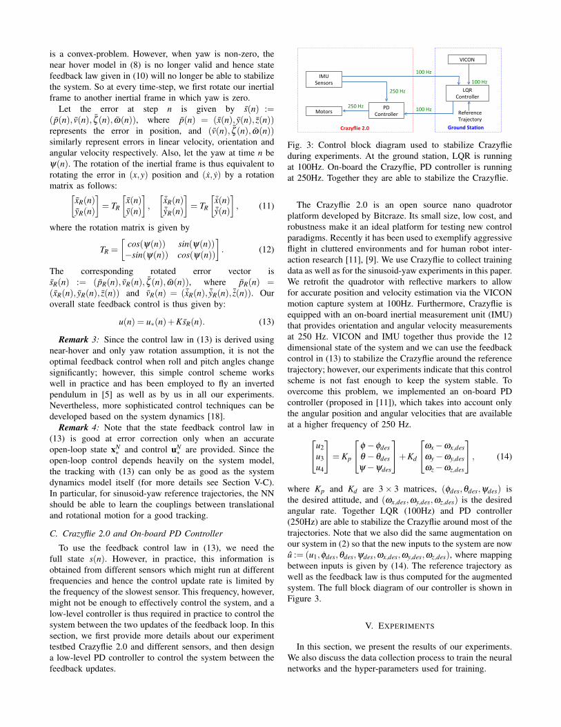
is a convex-problem. However, when yaw is non-zero, thenear hover model in (8) is no longer valid and hence statefeedback law given in (10) will no longer be able to stabilizethe system. So at every time-step, we first rotate our inertialframe to another inertial frame in which yaw is zero.

Let the error at step n is given by s(n) :=(p(n), v(n), ζ (n), ω(n)), where p(n) = (x(n), y(n), z(n))represents the error in position, and (v(n), ζ (n), ω(n))similarly represent errors in linear velocity, orientation andangular velocity respectively. Also, let the yaw at time n beψ(n). The rotation of the inertial frame is thus equivalent torotating the error in (x,y) position and (x, y) by a rotationmatrix as follows:[

xR(n)yR(n)

]= TR

[x(n)y(n)

],

[¯xR(n)¯yR(n)

]= TR

[¯x(n)¯y(n)

], (11)

where the rotation matrix is given by

TR =

[cos(ψ(n)) sin(ψ(n))−sin(ψ(n)) cos(ψ(n))

]. (12)

The corresponding rotated error vector issR(n) := (pR(n), vR(n), ζ (n), ω(n)), where pR(n) =(xR(n), yR(n), z(n)) and vR(n) = ( ¯xR(n), ¯yR(n), ¯z(n)). Ouroverall state feedback control is thus given by:

u(n) = u∗(n)+KsR(n). (13)

Remark 3: Since the control law in (13) is derived usingnear-hover and only yaw rotation assumption, it is not theoptimal feedback control when roll and pitch angles changesignificantly; however, this simple control scheme workswell in practice and has been employed to fly an invertedpendulum in [5] as well as by us in all our experiments.Nevertheless, more sophisticated control techniques can bedeveloped based on the system dynamics [18].

Remark 4: Note that the state feedback control law in(13) is good at error correction only when an accurateopen-loop state xN

∗ and control uN∗ are provided. Since the

open-loop control depends heavily on the system model,the tracking with (13) can only be as good as the systemdynamics model itself (for more details see Section V-C).In particular, for sinusoid-yaw reference trajectories, the NNshould be able to learn the couplings between translationaland rotational motion for a good tracking.

C. Crazyflie 2.0 and On-board PD Controller

To use the feedback control law in (13), we need thefull state s(n). However, in practice, this information isobtained from different sensors which might run at differentfrequencies and hence the control update rate is limited bythe frequency of the slowest sensor. This frequency, however,might not be enough to effectively control the system, and alow-level controller is thus required in practice to control thesystem between the two updates of the feedback loop. In thissection, we first provide more details about our experimenttestbed Crazyflie 2.0 and different sensors, and then designa low-level PD controller to control the system between thefeedback updates.

ControllerBlockDiagram

IMUSensors

LQRController

VICON

PDControllerMotors

Crazyflie2.0 GroundSta4on

100Hz

250Hz

250Hz 100Hz

100Hz

ReferenceTrajectory

Fig. 3: Control block diagram used to stabilize Crazyflieduring experiments. At the ground station, LQR is runningat 100Hz. On-board the Crazyflie, PD controller is runningat 250Hz. Together they are able to stabilize the Crazyflie.

The Crazyflie 2.0 is an open source nano quadrotorplatform developed by Bitcraze. Its small size, low cost, androbustness make it an ideal platform for testing new controlparadigms. Recently it has been used to exemplify aggressiveflight in cluttered environments and for human robot inter-action research [11], [9]. We use Crazyflie to collect trainingdata as well as for the sinusoid-yaw experiments in this paper.We retrofit the quadrotor with reflective markers to allowfor accurate position and velocity estimation via the VICONmotion capture system at 100Hz. Furthermore, Crazyflie isequipped with an on-board inertial measurement unit (IMU)that provides orientation and angular velocity measurementsat 250 Hz. VICON and IMU together thus provide the 12dimensional state of the system and we can use the feedbackcontrol in (13) to stabilize the Crazyflie around the referencetrajectory; however, our experiments indicate that this controlscheme is not fast enough to keep the system stable. Toovercome this problem, we implemented an on-board PDcontroller (proposed in [11]), which takes into account onlythe angular position and angular velocities that are availableat a higher frequency of 250 Hz.u2

u3u4

= Kp

φ −φdesθ −θdesψ−ψdes

+Kd

ωx−ωx,desωy−ωy,desωz−ωz,des

, (14)

where Kp and Kd are 3× 3 matrices, (φdes,θdes,ψdes) isthe desired attitude, and (ωx,des,ωy,des,ωz,des) is the desiredangular rate. Together LQR (100Hz) and PD controller(250Hz) are able to stabilize the Crazyflie around most of thetrajectories. Note that we also did the same augmentation onour system in (2) so that the new inputs to the system are nowu := (u1,φdes,θdes,ψdes,ωx,des,ωy,des,ωz,des), where mappingbetween inputs is given by (14). The reference trajectory aswell as the feedback law is thus computed for the augmentedsystem. The full block diagram of our controller is shown inFigure 3.

V. EXPERIMENTS

In this section, we present the results of our experiments.We also discuss the data collection process to train the neuralnetworks and the hyper-parameters used for training.

A. Data CollectionTo collect data for training, we flew Crazyflie au-

tonomously on a variety of trajectories, for example sinusoidsin XY, XZ and YZ planes (but no yaw), and fixed positionyaw-rotations, as well as manually on unstructured flights.For these flights, we recorded the state (s) and input (u) data.Note that since we do not necessarily care about how closelywe track a trajectory during the data collection process, thefeedback controller discussed in Section IV-B is sufficientto fly Crazyflie directly on the desired trajectories (that is,no feasible reference calculation is required); however, ingeneral, the entire data can also be collected manually withexperts flying the system.

A picture of Crazyflie flying during one of our experimentsis shown in Figure 1. One of our experimental videos can befound at: https://www.youtube.com/watch?v=QREeZvHg0lQ.For communication between the ground station andCrazyflie, we used the Robot Operating System (ROS)framework [15], [7]. In total there are 2400 seconds offlight time recorded, which correspond to 240,000 (s, u) datasamples. Note that since we augment the system with a PDcontroller, we collect u during the flights, as opposed to u.

B. Neural Network TrainingWe next train two NNs (denoted as NN1 and NN2 here

on) using the collected data to learn the linear and angularacceleration components fv and fω such that the MSE in (4)is minimized. Before training the NNs, we follow a few datapre-processing steps:• Since we collect u (input to the PD-augmented system),

we first derive u (input to the quadrotor system in (2))from u using (14), and use it as the input to the NNsalong with the state information. This is to make surethat the learned system dynamics are independent of thecontrol scheme.

• Instead of providing orientation angles as the input tothe NNs, we provide sines and cosines of the angles.This is to make sure that NNs do not differentiatebetween 0 and 2π radians.

• We do not provide position as the input to any ofthe neural networks, as the translational and rotationalaccelerations should be position independent.

• For each NN, we scale the observed outputs (for ex-ample, x,y,z components of translational acceleration)such that each of them has zero mean and unity standarddeviation. This is to make sure that the NNs give equalweightage to MSE in the three components.

The NN structure for each acceleration component is givenby (5). The objective (also called loss function) for each NNis to minimize the MSE between observed and predictedaccelerations. The input to NN1 is (v,ω,sin(ζ ),cos(ζ ),u1)and is (v,ω,sin(ζ ),cos(ζ ),u2,u3,u4) for NN2. Note thatwe do not include u2,u3,u4 in the input to NN1 becauseour experiments indicate that providing them result in over-fitting. Moreover, the physics of a quadrotor hints that thetranslational acceleration should not depend on these inputs[2]. The same argument holds for u1 and NN2.

0 2 4 6 8 10time(s)

-2

-1

0

1

2

Rol

l acc

eler

atio

n (ra

d/s2 ) Model Error

MeasuredNN output

0 2 4 6 8 10time(s)

-4

-2

0

2

4

Y ac

cele

ratio

n (m

/s2 )

Fig. 4: Observed and predicted values for the roll and yaccelerations. The NNs are able to learn the accelerationmodels fairly accurately even with just the current state andinput, indicating that the past states and inputs may not berequired to learn the dynamics, and hence are avoided in thiswork to keep the control design simple.

60% of the total collected data was used for training,25% was used for validation purposes and for tuning hyperparameters, and the rest was used for testing purposes. Allthe weights (W,w) and biases (B,b) were initially sampledfrom normal Gaussian distribution. For training the networks,we use the Neural Network Toolbox of MATLAB. Weuse the Resilient backpropagation learning algorithm. Thelearning rate, momentum constant, regularization factor andthe number of hidden units were set at 0.01, 0.95, 0.1and 100 respectively, but later tuned using the validationdata. Overall, the learning algorithm makes about 100 passesthrough the data, and optimize the weights and biases tominimize the loss function. Once the training is complete,the optimal weights and biases are obtained, which can besubstituted in (5) to obtain the models for fv and fω , andfinally in (2) to get the full dynamics model.

The (normalized) MSE numbers obtained for the trainingand the testing data after learning fv are 0.134 and 0.135respectively, and that for fω are 0.341 and 0.344. Sincethe MSE numbers are very close for training and testing,it indicates that the NNs do an accurate prediction on theunseen data as well, meaning that our NNs are not overfittingon the training data. In Figure 4, we show the observedvalues and the predicted outputs of the trained NNs for rolland y accelerations. As evident from the figure, the NNshave been successfully able to learn the dynamics to a goodaccuracy. This indicates that a simple two-layer feed-forwardNN structure used in this paper is sufficient to learn quadrotordynamics to a good accuracy. Moreover, only the currentstate and input information is sufficient to learn the dynamicsmodels, and hence past state and input information, whichwill potentially make the model as well as control designmore complex, has not been used as an input to the NNs.

C. Sinusoid-yaw Trajectory Tracking Using NN Models

Once NN1 and NN2 are trained, the full quadrotor modelis available through (2). In this section, our goal is to use thismodel to track a sinusoid-yaw trajectory, where quadrotoris undergoing a sinusoidal motion in the XY plane whileyawing at the same time. Since the desired trajectory consistsof a simultaneous translational and rotational movement, thelearned NN models should be able to capture the nonlinearcouplings between these two movements to accurately trackthe trajectory.

Using the full model, we first compute a dynamicallyfeasible reference that is as close as possible to the de-sired sinusoid-yaw trajectory (shown in Figure 5), usingthe sequential convex programming method outlined inSection IV-A. The reference trajectory is then flown us-ing the near-hover LQR scheme along with a yaw rota-tion as described in Section IV-B. One of the trackingvideos recorded during our experiments can be found at:https://www.youtube.com/watch?v=AeIfZbkjWPA. We labelthe results corresponding to this experiment as ‘NN model’trajectory.

The desired and NN model trajectories are shown in Figure5. As evident from the figure, the NN model trajectory is ableto track the desired trajectory closely. This illustrates that:• the trained NNs are able to generalize the dynamics

beyond the training data. In particular, the NN modelscapture the nonlinear couplings between translationaland rotational accelerations, and can be used to trackthe trajectories they were not trained on.

• even simple NN architectures, such as one used in thispaper, have good generalization capabilities and can beused to control a quadrotor on complex trajectories.

From the results thus far it is not clear how much ofthe control performance is due to the open-loop signalderived from the NN model, since the LQR control maybe correcting for model inconsistency. Therefore, we optedto fly Crazyflie using simply the LQR controller and desiredtrajectory as a reference and no open-loop control. We labelthe results corresponding to this experiment as the ‘model-free’ trajectory.

In Figure 6, we show the (absolute) tracking error for theNN model and model-free trajectories. The NN model hasa significantly lower tracking error compared to the model-free trajectory, indicating that the open-loop control derivedfrom the NN model results in better tracking of the desiredtrajectory. The reduced tracking error is thus the result ofthe availability of an accurate dynamics model. In general,to ensure a small tracking error, we need a good open-loopcontrol, which in turn need a good dynamics model thataccurately represents the system dynamics around the desiredtrajectory.

Our experiments thus indicate that given the state-inputdata of a complex dynamical system (quadrotors in our case),deep neural networks are capable of learning the systemdynamics to a good accuracy, and can represent the systembehavior beyond the data they were trained on. Moreover,

0 1 2 3 4time(s)

-1

0

1

2

3

x (m

)

0 1 2 3 4time(s)

-1

-0.5

0

0.5

1

y (m

)

0 1 2 3 4time(s)

-1.1

-1

-0.9

-0.8

z (m

)

0 1 2 3 4time(s)

-2

0

2

4

6

8

yaw

(rad

)

NN ModelModel FreeDesired

Fig. 5: The reference, NN model and model-free trajec-tories obtained during the experiments. The NN modeltrack the desired trajectory closely even though it involvesboth translational and rotational motion at the same time,which the NNs were not explicitly trained on, indicating thegeneralization capabilities of deep neural networks.

with a careful choice of the network architecture and itsinputs, the NN model can be used effectively to control thesystem. Thus, deep neural networks seem to present a goodalternative for the system identification of complex systemssuch as quadrotors, especially in scenarios in which it is hardto derive a physics-based model of the system.

Remark 5: Note that even though neural networks presentone approach to identify the complex system dynamics,it is not the only approach. In our experience, one canuse the general nonlinear model of quadrotor derived usingNewtonian-Euler formalism [2], [8] along with the controlscheme proposed in Section IV to get good tracking as well.Our goal in this paper, however, was to test the efficacyof neural network in learning a dynamic model, and not tocompare different system models. In practice, one can usethe physics-based model to collect data about the system andthen use a neural network to learn incremental unmodeleddynamics (on top of the physics-based model) which mightlead to an improved control performance.

VI. CONCLUSION

Traditional learning approaches proposed for controllingquadrotors have focused on improving the control perfor-mance for specific trajectories. In this work, we use deepneural networks to generalize the dynamics of the systembeyond the trajectories used for training. Our experimentsindicate that even simple NNs such as feed-forward net-works can also have good generalization capabilities and canlearn the dynamics of a quadrotor to good accuracy. Moreimportantly, we demonstrate that the learned dynamics canbe used effectively to control the system. Thus NNs are notonly useful in being a good function approximator, but in thisinstance we can actually exploit the function that it producesfor control purposes. For future work, it will be interesting

0 1 2 3 4time(s)

0

0.2

0.4

0.6

x er

ror (

m)

0 1 2 3 4time(s)

0

0.2

0.4

0.6

y er

ror (

m)

0 1 2 3 4time(s)

0

0.05

0.1

0.15

0.2

z er

ror (

m)

0 1 2 3 4time(s)

0

0.5

1

1.5

yaw

erro

r (ra

d)

NN ModelModel Free

Fig. 6: (Absolute) Tracking error for model-free and NNmodel trajectories. Model-free trajectory has a significantlyhigher tracking error compared to the NN model, especiallyin the translational motion, indicating that nonlinear couplingbetween translational and rotational motions should be takeninto account while designing a controller, which in this workis captured by training a NN model that accurately representsthe system dynamics.

to analyze whether combining a NN model with a physics-based model can lead to an improved control performance,thus utilizing both the known information about the systemas well as the generalization capabilities of NNs.

REFERENCES

[1] Pieter Abbeel, Adam Coates, and Andrew Y Ng. Autonomous heli-copter aerobatics through apprenticeship learning. The InternationalJournal of Robotics Research, 2010.

[2] Randal Beard. Quadrotor dynamics and control Rev 0.1. 2008.[3] Patrick Bouffard. On-board model predictive control of a quadrotor

helicopter: Design, implementation, and experiments. Technical report,DTIC Document, 2012.

[4] Eli Brookner. Tracking and kalman filtering made easy, John Wileyand Sons. Inc. NY, 1998.

[5] Markus Hehn and Raffaello D’Andrea. A flying inverted pendulum. InRobotics and Automation (ICRA), 2011 IEEE International Conferenceon, pages 763–770. IEEE, 2011.

[6] Markus Hehn and Raffaello DAndrea. An iterative learning schemefor high performance, periodic quadrocopter trajectories. In EuropeanControl Conference (ECC). IEEE, pages 1799–1804, 2013.

[7] Wolfgang Hoenig, Christina Milanes, Lisa Scaria, Thai Phan, MarkBolas, and Nora Ayanian. Mixed reality for robotics. In IEEE/RSJ IntlConf. Intelligent Robots and Systems, pages 5382 – 5387, Hamburg,Germany, Sept 2015.

[8] Gabriel M Hoffmann, Haomiao Huang, Steven L Waslander, andClaire J Tomlin. Quadrotor helicopter flight dynamics and control:Theory and experiment. In Proc. of the AIAA Guidance, Navigation,and Control Conference, volume 2, 2007.

[9] Wolfgang Honig, Christina Milanes, Lisa Scaria, Thai Phan, MarkBolas, and Nora Ayanian. Mixed reality for robotics. In IntelligentRobots and Systems (IROS), 2015 IEEE/RSJ International Conferenceon, pages 5382–5387. IEEE, 2015.

[10] Alex Krizhevsky, Ilya Sutskever, and Geoffrey E Hinton. Imagenetclassification with deep convolutional neural networks. In Advancesin neural information processing systems, pages 1097–1105, 2012.

[11] Benoit Landry. Planning and control for quadrotor flight throughcluttered environments. Master’s thesis, Massachusetts Institute ofTechnology, 2015.

[12] Yann LeCun, Yoshua Bengio, and Geoffrey Hinton. Deep learning.Nature, 521(7553):436–444, 2015.

[13] C Nicol, CJB Macnab, and A Ramirez-Serrano. Robust adaptivecontrol of a quadrotor helicopter. Mechatronics, 21(6):927–938, 2011.

[14] Ali Punjani and Pieter Abbeel. Deep learning helicopter dynamicsmodels. In Robotics and Automation (ICRA), 2015 IEEE InternationalConference on, pages 3223–3230. IEEE, 2015.

[15] Morgan Quigley, Ken Conley, Brian Gerkey, Josh Faust, Tully Foote,Jeremy Leibs, Rob Wheeler, and Andrew Y Ng. ROS: an open-sourcerobot operating system. In ICRA workshop on open source software,volume 3, page 5, 2009.

[16] Guilherme V Raffo, Manuel G Ortega, and Francisco R Rubio. Anintegral predictive/nonlinear H∞ control structure for a quadrotorhelicopter. Automatica, 46(1):29–39, 2010.

[17] J. B. Rawlings and D. Q. Mayne. Model predictive control: Theoryand design. Nob Hill Pub., 2009.

[18] Anand Sanchez-Orta, Vicente Parra-Vega, Carlos Izaguirre-Espinosa,and Octavio Garcia. Position–yaw tracking of quadrotors. Journal ofDynamic Systems, Measurement, and Control, 137(6):061011, 2015.

[19] John Schulman, Jonathan Ho, Alex X Lee, Ibrahim Awwal, HenryBradlow, and Pieter Abbeel. Finding locally optimal, collision-freetrajectories with sequential convex optimization. In Robotics: scienceand systems, volume 9, pages 1–10. Citeseer, 2013.

[20] Ilolger Voos. Nonlinear control of a quadrotor micro-UAV usingfeedback-linearization. In Mechatronics, 2009. ICM 2009. IEEEInternational Conference on, pages 1–6. IEEE, 2009.

[21] Eric A Wan and Ronell Van Der Merwe. The unscented kalman filterfor nonlinear estimation. In Adaptive Systems for Signal Processing,Communications, and Control Symposium 2000. AS-SPCC. The IEEE2000, pages 153–158. Ieee, 2000.

[22] Rong Xu and Umit Ozguner. Sliding mode control of a quadrotorhelicopter. In Decision and Control, 2006 45th IEEE Conference on,pages 4957–4962. IEEE, 2006.

[23] Ma Zhaowei, Hu Tianjiang, Shen Lincheng, Kong Weiwei, ZhaoBoxin, and Yao Kaidi. An iterative learning controller for quadrotorUAV path following at a constant altitude. In Control Conference(CCC), 2015 34th Chinese, pages 4406–4411. IEEE, 2015.