Learning Parts-Based Representations of Data - Department of

Journal of Machine Learning Research 7 (2006) 2369-2397 Submitted 2/05; Revised 10/06; Published 11/06

Learning Parts-Based Representations of Data

David A. Ross [email protected]

Richard S. Zemel [email protected]

Department of Computer ScienceUniversity of Toronto6 King’s College RoadToronto, Ontario M5S 3H5, CANADA

Editor: Pietro Perona

AbstractMany perceptual models and theories hinge on treating objects as a collection of constituent parts.When applying these approaches to data, a fundamental problem arises: how can we determinewhat are the parts? We attack this problem using learning, proposing a form of generative latentfactor model, in which each data dimension is allowed to select a different factor or part as its expla-nation. This approach permits a range of variations that posit different models for the appearance ofa part. Here we provide the details for two such models: a discrete and a continuous one. Further,we show that this latent factor model can be extended hierarchically to account for correlationsbetween the appearances of different parts. This permits modeling of data consisting of multiplecategories, and learning these categories simultaneously with the parts when they are unobserved.Experiments demonstrate the ability to learn parts-based representations, and categories, of facialimages and user-preference data.

Keywords: parts, unsupervised learning, latent factor models, collaborative filtering, hierarchicallearning

1. Introduction

Many collections of data exhibit a common underlying structure: they consist of a number of partsor factors, each with a range of possible states. When data are represented as vectors, parts manifestthemselves as subsets of the data dimensions that take on values in a coordinated fashion. In thedomain of digital images, these parts may correspond to the intuitive notion of the component partsof objects, such as the arms, legs, torso, and head of the human body. Prominent theories of compu-tational vision, such as Biederman’s Recognition-by-Components (Biederman, 1987) advocate thesuitability of a parts-based approach for recognition in both humans and machines. Recognizingan object by first recognizing its constituent parts, then validating their geometric configuration hasseveral advantages:

1. Highly articulate objects, such as the human body, are able to appear in a wide range ofconfigurations. It would be difficult to learn a holistic model capturing all of these variants.

2. Objects which are partially occluded can be identified as long as some of their parts arevisible.

c©2006 David A. Ross and Richard S. Zemel.

ROSS AND ZEMEL

3. The appearances of certain parts may vary less under a change in pose than the appearance ofthe whole object. This can result in detectors which, for example, are more robust to rotationsof the target object.

4. New examples from an object class may be recognized as simply a novel combination offamiliar parts. For example a parts-based face detection system could generalize to detectfaces with both beards and sunglasses, having been trained only on faces containing one, butnot both, of these features.

The principal difficulty in creating such systems is determining which parts should be used, andidentifying examples of these parts in the training data.

In the part-based detectors created by Mohan et al. (2001) and Heisele et al. (2000) partswere chosen by the experimenters based on intuition, and the component-detectors—support vec-tor machines—were trained on image subwindows containing only the part in question. Obtainingthese subwindows required that they be manually extracted from hundreds or thousands of train-ing images. In contrast, the parts-based detector created by Weber et al. (2000) proposed a way toautomate this process. During training of the geometric model, parts were selected from an initialset of candidates to include only those which lead to the highest detection performance. The re-sulting detector relied on a very small number of parts (e.g., 3) corresponding to very small localfeatures. Unlike the SVMs, which were trained on a range of appearances of the part, each of thesepart-detectors could identify only a single fixed appearance.

Parts-based representations of data can also be learned in an entirely unsupervised fashion.These parts can be used for subsequent supervised learning, but the models constructed can also bevaluable on their own. A parts-based model provides an efficient, distributed representation, andcan aid in the discovery of causal structure within data. For example, a model consisting of K parts,each with J possible states, can represent JK different objects. Inferring the state of each part canbe done efficiently, as each part depends only on a fraction of the data dimensions.

These computational considerations make parts-based models particularly suitable for modelinghigh-dimensional data such as user preferences in collaborative filtering problems. In this setting,each data vector contains ratings given by a human subject to a number of items, such as books ormovies. Typically there are thousands of unique items, but for each user we can only observe ratingsfor a small fraction of them. The goal in collaborative filtering is to make accurate predictions ofthe unobserved ratings. Parts can be formed from groups of related items, and the states of a partcorrespond to different attitudes towards the items. Unsupervised learning of a parts-based modelallows us to learn the relationships between items, which allows for efficient online and activelearning.

Here we propose a probabilistic generative approach to learning parts-based representations ofhigh-dimensional data. Our key assumption is that the dimensions of the data can be separatedinto several disjoint subsets, or factors, which take on values independently of each other. Eachfactor has a range of possible states or appearances, and we investigate two ways of modeling thisvariability. First we address the case in which each factor has a small number of discrete states, andmodel it using a vector quantizer. In some situations, however, continually-varying descriptionsof parts are more suitable. Thus, in our second approach we model part-appearances using factoranalysis. Given a set of training examples, our approach learns the association of data dimensionswith factors, as well as the states of each factor. Inference and learning are carried out efficientlyvia variational algorithms. The general approach, as well as details for the models, are given in

2370

LEARNING PARTS-BASED REPRESENTATIONS OF DATA

Section 2. Experiments showing parts-based representations learned for real data sets follow inSection 3.

Although we initially assume that parts take on states independently, clearly in real-world situ-ations there are dependencies. For example, consider the case of modeling images of human faces.A model could be constructed representing the various parts of the face (eyes, nose, mouth, etc.),and the various appearances of each part. If one part were to select an appearance with high pixelintensities, due to lighting conditions or skin tone, then it seems likely that the other parts shouldappear similarly bright. Realizing this, in Section 4 we propose a method of learning these depen-dencies between part selections hierarchically, by introducing an additional higher-level cause, or‘class’ variable, on which state selections for the factors are conditioned. This allows us to modeldifferent categories of data using the same vocabulary of parts, and to induce the categories whenthey are not available in advance. We conclude with a comparison to related methods, and a finaldiscussion in Sections 5 and 6.

2. An Approach to Learning Parts-Based Models

We approach the problem of learning parts by posing it as a stochastic generative model. We assumethat there are K factors, each a probabilistic model for the range of appearances of one of the parts.To generate an observed data vector of D dimensions, x ∈ ℜD, we stochastically select one statefor each factor, and one factor for each data dimension, xd . The first selection allows each part toindependently choose its appearance, while the second dictates how the parts combine to producethe observed data vector.

This approach differs from a traditional mixture model in that each dimension of the data is gen-erated by a different linear combination of the factors. Rather than clustering the data vectors basedon which mixture component gives the highest probability, we are grouping the data dimensionsbased on which part provides the best explanation.

The selection of factors for each dimension are represented as binary latent variables, R = rdk,for d = 1...D,k = 1...K. The variable rdk = 1 if and only if factor k has been selected for datadimension d. These variables can be described equivalently as multinomials, rd ∈ 1...K, and aredrawn according to their respective prior distributions, P(rdk) = adk. The choice of state for eachfactor is also a latent variable, which we will represent by sk. Using θk to represent the parametersof the kth factor, we arrive at the following complete likelihood function:

P(x,R,S|θ) = ∏d,k

(adkrdk)∏

k

(P(sk))∏d,k

(P(xd |θk,sk)rdk) . (1)

This probability model is depicted graphically in Figure 1.As described thus far, the approach is independent of the particular choice of model used for

each of the factors. We now provide details for two particular choices: a discrete model of factors,vector quantization; and a continuous model, factor analysis.

2.1 Multiple Cause Vector Quantization

In Multiple Cause Vector Quantization, first proposed in Ross and Zemel (2003), we assume thateach part has a small number of appearances, and model them using a vector quantizer (VQ) of Jpossible states. To generate an observed data example, we stochastically select one state for each

2371

ROSS AND ZEMEL

xdda kbksdr

θkD

K

Figure 1: Graphical representation of the parts-based learning model. We let rd=1 represent all thevariables rd=1,k, which together select a factor for x1. Similarly, sk=1 selects a state forfactor 1. The plates depict repetitions across the D input dimensions and the K factors.To extend this model to multiple data cases, we would include an additional plate over r,x, and s.

VQ, and, as described above, one VQ for each dimension. Given these selections, a single statefrom a single VQ determines the value of each data dimension xd .

As before, we represent the selections using binary latent variables, S = sk j, for k = 1...K, j =1...J, where sk j = 1 if and only if state j is selected for VQ k. Again we introduce prior selectionprobabilities P(sk j) = bk j, with ∑ j bk j = 1.

Assuming each VQ state specifies the mean as well as the standard deviation of a Gaussiandistribution, and the noise in the data dimensions is conditionally independent, we have (whereθk = µdk j,σdk j, and N is the Gaussian pdf)

P(x|R,S,θ) = ∏d,k, j

N (xd ; µdk j, σ2dk j)

rdk sk j .

The resulting model can be thought of as a Gaussian mixture model over J×K possible statesfor each data dimension (xd). The single state k j is selected if sk jrdk = 1. Note that this selection hastwo components. The selection in the j component is made jointly for the different data dimensions,and in the k component it is made independently for each dimension.

2.1.1 LEARNING AND INFERENCE

The joint distribution over the observed vector x and the latent variables is

P(x,R,S|θ) = P(R|θ)P(S|θ)P(x|R,S,θ),

= ∏d,k

(

ardkdk

)

∏k, j

(

bsk j

k j

)

∏d,k, j

N (xd ; θk)rdksk j .

Given an input x, the posterior distribution over the latent variables, P(R,S|x,θ), cannot tractablybe computed, since all the latent variables become dependent.

We apply a variational EM algorithm to learn the parameters θ, and infer latent variables givenobservations. For a given observation, we could approximate the posterior distribution using afactored distribution, where g and m are variational parameters related to r and s respectively:

Q0(R,S|x,θ) = ∏d,k

(

grdkdk

)

∏k, j

(

msk j

k j

)

. (2)

2372


The model is learned by optimizing the following objective function (Neal and Hinton, 1998),also known as the variational free energy:

F (Q0,θ) = EQ0 [logP(x,R,S|θ)− logQ0(R,S|x,θk)] ,

= EQ0

[

−∑d,k

rdk log(gdk/adk)−∑k, j

sk j log(mk j/bk j)+ ∑d,k, j

rdksk j logN (xd ; θ)

]

,

= −∑d,k

gdk loggdk

adk−∑

k, j

mk j logmk j

bk j− ∑

d,k, j

gdk mk j εdk j,

where εdk j = logσdk j +(xd−µdk j)

2

2σ2dk j

. The objective function F is a lower bound on the log likelihood

of generating the observations, given the particular model parameters. The variational EM algorithmimproves this bound by iteratively maximizing F with respect to Q0 (E-step) and to θ (M-step).

Extending this to handle multiple observations—the columns of X = [x1 . . .xC]—we must nowconsider approximating the posterior P(R ,S |X,θ), where R = rc

dk and S = sck j are the latent

selections for all training cases c. Our aim is to learn models which have a posterior distribution overfactor selections for each data dimension that is consistent across all data (that is to say, regardlessof the data case, each xd will typically be associated with the same part or parts). Thus, in thevariational posterior we constrain the parameters gdk to be the same across all observations xc,c =1 . . .C. In this general case, the variational approximation to the posterior becomes (cf. Equation (2))

Q(R ,S |X,θ) = ∏c,d,k

(

gdkrc

dk

)

∏c,k, j

(

mck j

sck j

)

. (3)

It is important to point out that this choice of variational approximation is somewhat unorthodox,nonetheless it is perfectly valid and has produced good results in practice. A comparison to moreconventional alternatives appears in Appendix A.

Under this formulation, only the mck j parameters are updated during the E step for each ob-

servation xc:

mck j = bk j exp

(

−∑d

gdk εcdk j

)

/J

∑ρ=1

bkρ exp(

−∑d

gdk εcdρk

)

.

The M step updates the parameters, µ and σ, which relate each latent state k j to each inputdimension d, the parameters of Q related to factor selection gdk, and the priors adk and bk j:

gdk = adk exp(

−1C ∑

c, j

mck j εc

dk j

)

/K

∑ρ=1

adρ exp(

−1C ∑

c, j

mcjρ εc

d jρ

)

, (4)

µdk j =∑c mc

k jxcd

∑c mck j

, σ2dk j =

∑c mck j(x

cd−µdk j)

2

∑c mck j

,

adk = gdk, bk j =1C ∑

cmc

k j.

As can be seen from the update equations, an iteration of EM learning for MCVQ has compu-tational complexity linear in each of C, D, J, and K.

2373

ROSS AND ZEMEL

A variational approximation is just one of a number of possible approaches to performing theintractable inference (E) step in MCVQ. One alternative, known as Monte Carlo EM, is to approxi-mate the posterior with a set of samples Rn,Sn

Nn=1 drawn from the true posterior P(R ,S |X,θ)

via Gibbs sampling. The M step now becomes a maximization of the approximate likelihood1N ∑n P(X,Rn,Sn|θ) with respect to the model parameters θ. Note that the intractable marginal-ization over rc

dk,sck j has been replaced with the less-costly sum over N samples. Details of this

approach for a related model can be found in Ghahramani (1995), and a general description inAndrieu et al. (2003).

2.2 Multiple Cause Factor Analysis

In MCVQ, each factor is modeled as a set of basis vectors, one of which is chosen at a time whengenerating data. A more general approach is to allow data to be generated by arbitrary linear com-binations of the basis vectors in each factor. This extension (with the appropriate choice of priordistribution) amounts to modeling the range of appearances for each part with a factor analyzer.

A factor analysis (FA) model (e.g., Ghahramani and Hinton, 1996) proposes that the data vectorscome from a low-dimensional linear subspace, represented by the basis vectors of the factor loadingmatrix, Λ∈ℜD×J , and an offset ρ∈ℜD from the origin. A data vector is produced by taking a linearcombination s ∈ℜJ of the columns of Λ. The linear combination is treated as an unobserved latentvariable, with a standard Gaussian prior P(s) = N (s;0,I). To this is added zero-mean Gaussiannoise, independent along each dimension. The probability model is

P(x,s|θ) = N (x;Λs+ρ,Ψ) N (s;0,I) (5)

where Ψ is a D×D diagonal covariance matrix.As with MCVQ, we assume that the data contains K parts and model each using a factor analyzer

θk = (Λk,ρk,Ψk). A data vector is again generated by stochastically selecting one state sk per factork, and choosing one factor per data dimension. Under this model factor analyzer k proposes that thevalue of xd has a Gaussian distribution centered at Λk

dsk +ρdk with variance Ψkd (where Λk

d indicatesthe dth row of factor loading matrix k, and Ψk

d the dth entry on the diagonal of Ψk). Thus thelikelihood is

P(x|R,S,θ) = ∏d,k

N (xd ;Λkdsk +ρdk,Ψk

d)rdk .

2.2.1 LEARNING AND INFERENCE

Again this model produces an intractable posterior over latent variables S and R, so we resort to avariational approximation:

Q(R ,S |X,θ) = ∏c,d,k

(

grc

dkdk

)

∏c,k

N (sck;mc

k,Ωck).

This differs from the approximation used for MCVQ, Equation (3), in that here we assume the statevariables sk have Gaussian posteriors. Thus, in the E step we must now estimate the first and secondmoments of the posterior over sk. As before, we also tie the gdk parameters to be the same acrossall data cases. Setting up the objective function and differentiating, gives us the following updates

2374


for the E-step:1

mck = ΩckΛkT Ψ−1

k ((xc−ρk) .∗gk),

Ωck =(

ΛkT gk

Ψk Λk + I)−1

, 〈scksc

kT 〉= Ωck +mc

kmck

T ,

where gkΨk is a diagonal matrix with entries gdk/Ψk

d . Note that the expression for Ωck is independentof the index over training cases, c, thus we need only have one Ωk = Ωck,∀c.

The M-step involves updating the prior and variational posterior factor-selection parameters,adk and gdk, as well as the parameters (Λk,ρk,Ψk) of each factor analyzer. At each iterationthe prior, adk = gdk is set to the posterior at the previous iteration. The remaining updates are

gdk ∝adk

|Ψkd|

1/2exp

[

−1

2CΨkd∑c

(

(xcd−ρdk)

2 +Λkd〈s

cksc

kT 〉Λk

dT−2(xc

d−ρdk)Λkdmc

k

)

]

,

Λk =(

X−ρk1T )MT

k

(

∑c〈sc

ksck

T 〉

)−1

,

ρk =1C ∑

c

(

xc−Λkmck

)

,

Ψkd =

1C ∑

c

(

(xcd−ρdk)

2 +Λkd〈s

cksc

kT 〉Λk

dT−2(xc

d−ρdk)Λkdmc

k

)

.

where (Mk is a J×C matrix in which the cth column is mck).

2.3 Related Algorithms

Here we present the details of two related algorithms, principal components analysis (PCA), andnon-negative matrix factorization (NMF). A more detailed comparison of these algorithms withMCVQ and MCFA appears below, in Section 5.

The goal of PCA is to learn a factorization of the data matrix X into the product of a coefficientmatrix S and an orthogonal basis Λ so that X≈ ΛS. Typically Λ has fewer columns than rows, so Scan be thought of as a reduced-dimensionality approximation of X, and Λ as the key features of thedata. Using a squared-error cost function, the optimal solution is to let Λ be the top eigenvectors ofthe sample covariance matrix, 1

C−1 XXT , and let S = ΛT X.PCA can also be posed as a probabilistic generative model, closely related to factor analysis

(Roweis, 1997; Tipping and Bishop, 1999). In fact, probabilistic PCA proposes the same generativemodel, Equation (5), except that the noise covariance, Ψ, is restricted to be a scalar times the identitymatrix: Ψ = σ2I.

Non-negative matrix factorization (Lee and Seung, 1999) also learns a factorization X ≈WHof the data matrix, but includes the additional restriction that X, W, and H must be entirely non-negative. By allowing only additive combinations of a non-negative basis, Lee & Seung proposeto obtain basis vectors that correspond to the intuitive parts of the data. Instead of squared error,NMF seeks to minimize the divergence D(X‖WH) = ∑d,c

[

xcd log(WH)dc− (WH)dc

]

which is the

1. The second uncentered moment 〈scksc

kT 〉 need not be computed explicitly, since it can be expressed as a combination

of the first and second centered moments, mk and Ωck. It is, however, a useful subexpression for computing theM-step updates and likelihood bound.

2375

ROSS AND ZEMEL

negative log-probability of the data, assuming a Poisson density function with mean WH. A localminimum of the divergence is obtained by iterating the following multiplicative updates:

wd j← wd j ∑c

xcd

(WH)dch jc, wd j←

wd j

∑d′ wd′ j, h jc← h jc ∑

d

wd jxc

d

(WH)dc.

Despite the probabilistic interpretation, X ∼ Poisson(WH), NMF is not a proper probabilisticgenerative model, since it does not specify a prior distribution over the latent variable H. Thus NMFdoes not specify how new data could be generated from a learned basis.

Like the above methods, MCVQ and MCFA can be viewed as matrix factorization methods,where the left-hand matrix is formed from the gdk and the collection of VQ/FA basis vectors,while the right-hand matrix is comprised of the latent variables mc

k j. This view highlights the keycontrast between the assumptions about the data embodied in these earlier models, as opposed to theproposed model. Here the data is viewed as a concatenation of components or parts, correspondingto particular subsets of data dimensions, each of which is modeled as a convex combination ofappearances.

3. Experiments

In this section we examine the ability of MCVQ and MCFA to learn parts-based representations ofdata from two different problem domains.

We begin by modeling sets of digital images, in this case images of human faces. The partslearned are fixed subsets of the data dimensions (pixels), corresponding to fixed regions of theimages, that closely resemble intuitive notions of the parts of faces. The ability to learn parts isrobust to partial occlusions in the training images.

The application of MCVQ and MCFA to image data assumes that the images are normalized,that is, that the head is in a similar pose in each image, and aligned with respect to position andscale. This constraint is standard for learning methods that attempt to learn visual features beyondlow level edges and corners, though, if desired, the model could be extended to perform automaticalignment of images (Jojic and Caspi, 2004). While normalization may require a preprocessing stepfor image applications, in many other types of applications, the input representation is more stable.For instance, in collaborative filtering each data vector consists of a single user’s ratings for a fixedset of items; each data dimension always corresponds to the same item.

Thus, we also explore the application of MCVQ and MCFA to the problem of predicting ratingsof unseen movies, given observed ratings for a large set of users. Here parts correspond to subsetsof the movies which have correlated ratings.

Code implementing MCVQ and MCFA in MATLAB, as used for the following experiments, canbe obtained at http://www.cs.toronto.edu/∼dross/mcvq/.

3.1 Face Images

The face data set consisted of 2429 images from the CBCL Face database #1 (MIT-CBCL, 2000).Each image contained a single frontal or near-frontal face, depicted in 19×19 pixel grayscale. Theimages were histogram equalized, and pixel values rescaled to lie in [−2,2]. Sample training imagesare shown in Figure 2.

Using these images as input, we trained MCVQ and MCFA models, each containing K = 6factors. The MCVQ model with J = 10 states converged in 120 iterations of Monte Carlo EM, while

2376


Figure 2: Sample training images from the CBCL Face database #1.

VQ 1

VQ 2

VQ 3

VQ 4

VQ 5

VQ 6

Figure 3: The parts-based model of faces learned by MCVQ. On the left are plots showing theposterior probability with which each pixel selects the indicated VQ. On the right are themeans, for each state of each VQ, masked by the aforementioned selection probabilities(µk j .∗gk).

the MCFA model with J = 4 basis vectors converged in 15 variational EM iterations. In practice, theMonte Carlo approach to inference leads to better local maxima of the objective function, and betterparts-based models of the data. For both MCVQ and MCFA, prior probabilities were initializedto uniform, and states/basis vectors to randomly selected training images. The learned parts-baseddecompositions are depicted in Figures 3 and 4.

On the left of each figure is a plot of posterior probabilities gdk that each pixel selects theindicated factor as its explanation. White indicates high probability of selection, and black low. Ascan be seen, each gk can be thought of as a mask indicating which pixels ‘belong’ to factor k.

In the noise-free case, each image generated by one of these models is a sum of the contributionsfrom the various factors, where each contribution is ‘masked’ by the probability of pixel selection.For example in Figure 3 the probability of selecting VQ #4 is non-zero only around the nose, thusthe contribution of this VQ to the remaining areas of the face in any generated image is negligible.

On the right of each figure is a plot of the 10 states/4 basis vectors for each factor. Each imagehas been masked (via element-wise multiplication) with the corresponding gk. For MCVQ this is(µdk j .∗gdk), and for MCFA this is (Λk

d j .∗gdk). In the case of MCVQ, each state is an alternativeappearance for the corresponding part. For example VQ #4 gives 10 alternative noses to select from

2377

ROSS AND ZEMEL

FA 1

FA 2

FA 3

FA 4

FA 5

FA 6

Figure 4: The parts-based model of faces learned by MCFA.

when generating a face. These range from thin to wide, with shadows of the left or right, and withlight or dark upper-lips (possibly corresponding to moustaches). In MCFA, on the other hand, thebasis vectors are not discrete alternatives. Rather these vectors are combined via arbitrary linearcombinations to generate an appearance of a part.

To test the fidelity of the learned representations, the trained models were used to probabilisti-cally classify held-out test images as either face or non-face. The test data consisted of the 472 faceimages and 472 randomly-selected non-face images from the CBCL database test set. To classifytest images, we evaluated their probability under the model, labeling an image as face if its prob-ability exceeded a threshold, and non-face if it did not. For each model the threshold was chosento maximize classification performance. Evaluating the probability of a data vector under MCVQand MCFA can be difficult, since it requires marginalizing over all possible values of the latent vari-ables. Thus, in practice, we use a Monte Carlo approximation, obtained by averaging over a sampleof possible selections. The results of this experiment are shown in Table 1. In addition to MCVQand MCFA, we performed the same experiment with four other probabilistic models: probabilisticprincipal components analysis (PPCA), mixture of Gaussians, a single Gaussian distribution, andcooperative vector quantization (Hinton and Zemel, 1994) (which is described further in Section 5).It is important to note that in this experiment an increase in model size (using more VQs, states,or basis vectors) does not necessarily improve the ability to discriminate faces from non-faces. Forexample, PPCA achieves its highest accuracy when using only three basis vectors, and a mixture ofGaussians with 60 states outperforms one with 84 states. As can be seen, the highest performanceis achieved by an MCVQ model with 6 VQs and 14 states per VQ.

Another way of validating image models it to use them to generate new examples and see howclosely they resemble images from the observed data—in this case how much the generated im-ages resemble actual faces. Examples of images generated from MCVQ and MCFA are shown inFigure 5.

2378


Model AccuracyMCVQ (6 VQs, 14 states each) 0.8305Mixture of Gaussians (60 states) 0.8072MCVQ (6 VQs, 10 states each) 0.8030Probabilistic PCA (3 components) 0.7903Gaussian distribution (diagonal covariance) 0.7871Mixture of Gaussians (84 states) 0.7680MCFA (6 FAs, 3 basis vectors each) 0.7415MCFA (6 FAs, 4 basis vectors each) 0.7267Cooperative Vector Quantization (6 VQs, 10 states each) 0.6208

Table 1: Results of classifying test images as face or non-face, by computing their probabilitiesunder trained generative models of faces.

Figure 5: Synthetic images generated using MCVQ (left) and MCFA (right).

The parts-based models learned by MCVQ and MCFA differ from those learned by NMF andPCA, as depicted in Figure 6, in two important ways. First, the basis is sparse—each factor con-tributes to only a limited region of the image, whereas in NMF and PCA basis vectors includemore global effects. Secondly MCVQ and MCFA learn a grouping of vectors into related parts, byexplicitly modeling the sparsity via the gdk distributions.

A further point of comparison is that, in images generated by PPCA and NMF, a significantproportion of the pixels in the generated images lie outside the range of values appearing in thetraining data (7% for PPCA and 4.5% for NMF), requiring that the generated values be thresholded.On the other hand, MCVQ will never generate pixel values outside the observed range. This is asimple result, since each generated image is a convex combination of basis vectors, and each basisvector is a convex combination of data vectors. Although no such guarantee exists for MCFA, inpractice pixels it generates are all within-range.

2379

ROSS AND ZEMEL

Figure 6: Bases learned by non-negative matrix factorization (left) and probabilistic principal com-ponents analysis (right), when trained on the face images.

3.1.1 PARTIAL OCCLUSION

Parts-based models can also be reliably learned from image data in which the object is partiallyoccluded. As an illustration, we trained an MCVQ model on a data set containing partially-occludedfaces. The occlusions were generated by replacing pixels in randomly-selected contiguous regionsof each training image with noise. The noise, which covered 1

4 to 12 of each image, had the same

first- and second-order statistics as the unoccluded pixels. The resulting training set contained 4858images, half of which were partially occluded.

Examples of the training images, and the resulting model, can be seen in Figure 7. In the modeleach VQ has learned at least one state containing a blurry region, which corresponds to an occludedview of the respective part (e.g., for VQ 1, the second state from the right). Thus this model is ableto generate and reconstruct (recognize) partially-occluded faces.

3.2 Collaborative Filtering

Here we test MCVQ on a collaborative filtering task, using the EachMovie data set, where theinput vectors are ratings by viewers of movies, and a given element always corresponds to the samemovie. The original data set contains ratings, on a scale from 1 to 6, of a set of 1649 movies, by74,424 viewers. In order to reduce the sparseness of the data set, since many viewers rated only afew movies, we only included viewers who rated at least 20 movies, and removed unrated movies.The remaining data set, containing 1623 movies and 36,656 viewers, was still very sparse (95.7%).

We evaluated the performance of MCVQ using the framework proposed by Marlin (2004) forcomparison of collaborative filtering algorithms. From each viewer in the EachMovie set, a singlerandomly-chosen rating was held out. The performance of the model at predicting these held-outratings was evaluated using 3-fold cross validation. In each fold, the model was fit to a training set

2380


VQ 1

VQ 2

VQ 3

VQ 4

VQ 5

VQ 6

Figure 7: The model learned by MCVQ on partially-occluded faces. On the left are six representa-tive images from the training data. In the middle are plots of the posterior part selectionprobability (the gdk’s) for each VQ. On the right are the (unmasked) means for each stateof each VQ. Note that each VQ has learned at least one state to represent partial occlusionof the corresponding part.

of 2/3 of the viewers, with the remaining 1/3 viewers retained as a testing set.2 This model was usedto predict the held-out ratings of the training viewers, a task referred to as weak generalization, aswell as the held-out ratings of the testing viewers, called strong generalization. Each prediction wasobtained by first inferring the latent states of the factors mk j, then averaging the mean of each stateby its probability of selection: ∑k, j gdk mk j µk jd .

Prediction performance was calculated using normalized mean absolute error (NMAE). Givena set of predictions pi, and the corresponding ratings ri, the NMAE is

1zn

n

∑i=1

|ri− pi|

where z is a normalizing factor equal to the expectation of the mean absolute error, assuminguniformly distributed pi’s and ri’s (Marlin, 2004).3 For the EachMovie data set this value isz = 35/18≈ 1.9444.

We trained several models on this data set, including MCVQ, MCFA, factor analysis, mixtureof Gaussians, as well as a baseline algorithm which, for each movie, simply predicts the mean of

2. This differs slightly from Marlin’s approach. He used three randomly sampled training and test sets of 30000 and5000 viewers respectively. However, his test sets were not disjoint, introducing a potential bias in the error estimate.We, instead, partitioned the data into thirds, using 2/3 of the viewers for training and 1/3 for testing in each of thethree folds. The resulting estimates of error should be less biased, but remain directly comparable to Marlin’s results.

3. For data sets in which the ratings range over the integers, from a minimum of m to a maximum of M, there is a simple

expression for z. Let N = M−m be the largest possible absolute error. Then z =N(N+2)3(N+1)

.

2381

ROSS AND ZEMEL

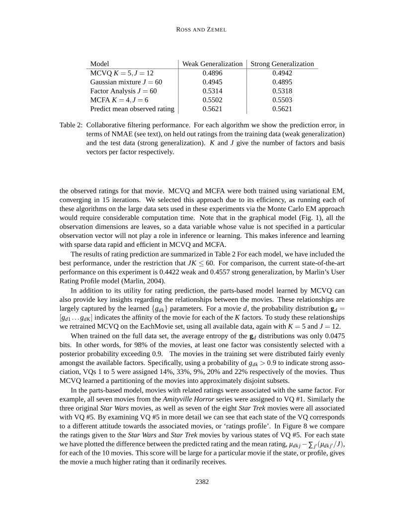
Model Weak Generalization Strong GeneralizationMCVQ K = 5,J = 12 0.4896 0.4942Gaussian mixture J = 60 0.4945 0.4895Factor Analysis J = 60 0.5314 0.5318MCFA K = 4,J = 6 0.5502 0.5503Predict mean observed rating 0.5621 0.5621

Table 2: Collaborative filtering performance. For each algorithm we show the prediction error, interms of NMAE (see text), on held out ratings from the training data (weak generalization)and the test data (strong generalization). K and J give the number of factors and basisvectors per factor respectively.

the observed ratings for that movie. MCVQ and MCFA were both trained using variational EM,converging in 15 iterations. We selected this approach due to its efficiency, as running each ofthese algorithms on the large data sets used in these experiments via the Monte Carlo EM approachwould require considerable computation time. Note that in the graphical model (Fig. 1), all theobservation dimensions are leaves, so a data variable whose value is not specified in a particularobservation vector will not play a role in inference or learning. This makes inference and learningwith sparse data rapid and efficient in MCVQ and MCFA.

The results of rating prediction are summarized in Table 2 For each model, we have included thebest performance, under the restriction that JK ≤ 60. For comparison, the current state-of-the-artperformance on this experiment is 0.4422 weak and 0.4557 strong generalization, by Marlin’s UserRating Profile model (Marlin, 2004).

In addition to its utility for rating prediction, the parts-based model learned by MCVQ canalso provide key insights regarding the relationships between the movies. These relationships arelargely captured by the learned gdk parameters. For a movie d, the probability distribution gd =[gd1 . . .gdK ] indicates the affinity of the movie for each of the K factors. To study these relationshipswe retrained MCVQ on the EachMovie set, using all available data, again with K = 5 and J = 12.

When trained on the full data set, the average entropy of the gd distributions was only 0.0475bits. In other words, for 98% of the movies, at least one factor was consistently selected with aposterior probability exceeding 0.9. The movies in the training set were distributed fairly evenlyamongst the available factors. Specifically, using a probability of gdk > 0.9 to indicate strong asso-ciation, VQs 1 to 5 were assigned 14%, 33%, 9%, 20% and 22% respectively of the movies. ThusMCVQ learned a partitioning of the movies into approximately disjoint subsets.

In the parts-based model, movies with related ratings were associated with the same factor. Forexample, all seven movies from the Amityville Horror series were assigned to VQ #1. Similarly thethree original Star Wars movies, as well as seven of the eight Star Trek movies were all associatedwith VQ #5. By examining VQ #5 in more detail we can see that each state of the VQ correspondsto a different attitude towards the associated movies, or ‘ratings profile’. In Figure 8 we comparethe ratings given to the Star Wars and Star Trek movies by various states of VQ #5. For each statewe have plotted the difference between the predicted rating and the mean rating, µdk j−∑ j′(µdk j′/J),for each of the 10 movies. This score will be large for a particular movie if the state, or profile, givesthe movie a much higher rating than it ordinarily receives.

2382


The four states depicted in Figure 8 show a range of possible ratings profiles. State 2 shows astrong preference for all the movies, with each receiving a rating 1-2.5 points higher than usual. Incontrast, state 9 shows an equally strong dislike for the movies. State 10 indicates a viewer who isfond of Star Wars, but not Star Trek. Finally, state 11 shows an ambivalent attitude: slight preferencefor some films, and slight dislike for others.

W1 W2 W3 T1 T2 T3 T4 T5 T6 T7−2.5

0

2.5VQ 5, State 2

W1 W2 W3 T1 T2 T3 T4 T5 T6 T7−2.5

0

2.5VQ 5, State 9

W1 W2 W3 T1 T2 T3 T4 T5 T6 T7−2.5

0

2.5VQ 5, State 10

W1 W2 W3 T1 T2 T3 T4 T5 T6 T7−2.5

0

2.5VQ 5, State 11

Star Wars W1 Star Trek III: The Search for Spock T3The Empire Strikes Back W2 Star Trek IV: The Voyage Home T4Return of the Jedi W3 Star Trek V: The Final Frontier T5Star Trek: The Motion Picture T1 Star Trek VI: The Undiscovered Country T6Star Trek II: The Wrath of Khan T2 Star Trek: First Contact T7

Figure 8: Ratings profiles learned by MCVQ on the EachMovie data, for Star Wars and Star Trekmovies. Each state represents a different attitude towards the movies. Positive scorescorrespond to above-average ratings for the movie, and negative to below-average.

3.2.1 ACTIVE LEARNING

When collaborative filtering is posed in an online or active setting, the set of available data is con-tinually growing, as viewers are queried and new ratings are observed. When a viewer provides anew rating for an item, the system’s beliefs about his preferences must be updated. In generativemodels, such as we have described, this entails updating the distribution over latent state variablesfor the viewer. This update is often costly, and can pose a problem when the system must be usedinteractively. Furthermore, queries of the sort “What is the rating of xd?” must be generated online,based on the viewer’s previous responses, to maximize the value of the information obtained. This

2383

ROSS AND ZEMEL

value could simply be the system’s certainty as to the viewer’s preferences, or, more interestingly,its ability to recommend movies that he might enjoy.

The parts based models we describe significantly simplify both of these computations. Bylearning a partitioning of the items, a new rating will only affect beliefs about unobserved ratingsassociated with the same factor. Specifically, only one mk j will be updated for each new rating, andthe update will depend only on a fraction of the observations.

Also, since we explicitly model the relationships between items, we can determine how thepossible responses to a putative query would affect predictions. Thus, we can formulate a querydesigned to identify movies with high predicted ratings. More details on a successful application ofMCVQ to active collaborative filtering, using these ideas, can be found in Boutilier et al. (2003).

4. Hierarchical Learning

Thus far it has been assumed that the states of each factor are selected independently. Althoughthis assumption has proven useful, it is unrealistic to suppose that, for example, the appearance ofthe eyes and mouth in a face are entirely uncorrelated. Rather than simply being a violation of ourmodeling assumptions, these correlations can be viewed as an additional source of information fromwhich we can learn higher-order structure present in the data.

Here we relax the assumption of independence by including an additional higher-level latentvariable upon which state selections are conditioned. This variable has two possible interpretations.First, if the higher-level cause is unobserved, it can be learned, inducing a categorization of the datavectors based on their state selections. Secondly, if the variable is observed, it can be treated as sideinformation available during learning. In this case the prior over state selections will be adapted toaccount for the side information.

We now develop both approaches, and demonstrate their use on a set of images containingdifferent facial expressions.

4.1 Extending the Generative Model

Suppose that each data vector comes from one of N different classes. We assume that for a givendata vector the selections of the states for each factor (the sk’s) depend on the class, but that theselections of a factor per data dimension (the rd’s) do not. Specifically, for training case x, weintroduce a new multinomial variable y which selects exactly one of the N classes. y can be thoughtof as an indicator vector y ∈ 0,1N , where yn = 1 if and only if class n has been selected. Using aprior P(yn = 1) = βn over y, the complete likelihood takes the following form (cf. Equation (1)):

P(x,R,S,y|θ) = P(x|R,S,θ)P(R)P(S|y)P(y),

= ∏d,k

(P(xd|θk,sk)rdk)∏

d,k

(

ardkdk

)

∏n,k, j

(

bsk jyn

nk j

)

∏n

(βynn ) . (6)

The graphical model representation is given in Figure 9.Note that for each class n there is a different prior distribution over the state selections. We

represent these distributions with bnk jnk j, ∑ j bnk j = 1, where bnk j is the probability of selectingstate j from factor k given class n. Since the model contains N priors over S, one to be selected foreach data vector, then we can think of this model as incorporating an additional vector quantizationor clustering, this time over distributions for S.

2384


βxdda ksdr

θkD

K

y

Figure 9: Graphical model with additional class variable, y. Note that y can be either observed orunobserved.

If the class variable y corresponds to an observed label for each data vector, then the new modelcan be thought of as a standard MCVQ or MCFA model, but with the requirement that we learna different prior over S for each class. On the other hand, if y is unobserved, then the new modellearns a mixture over the space of possible priors for S, rather than the single maximum likelihoodpoint estimate learned in standard MCVQ and MCFA.

Below we derive the EM updates for the hierarchical MCVQ model. The derivation of hierar-chical MCFA is similar.

4.2 Unsupervised Case

In the unsupervised case, yc, for each training case c = 1 . . .C is an unobserved variable, like Rc

and Sc. As in standard MCVQ, the posterior P(R,S,y|x,θ) over latent variables cannot tractably becomputed. Instead, we use the following factorized variational approximation:

Q(R ,S ,Y ) =

(

∏c,d,k

grc

dkdk

)(

∏c,n,k, j

mcnk j

sck jy

cn

)(

∏c,n

zcn

ycn

)

.

Note that, as in standard MCVQ, we restrict the posterior selections of VQ made for eachtraining case to be identical, that is, gdk is independent of c. Using the variational posterior andthe likelihood, Equation (6), we obtain the following lower bound on the log-likelihood:

F = EQ [logP(X ,R ,S ,Y |θ)− logQ(R ,S ,Y |X,θ))] ,

= EQ

[

∑c

logP(xc|Rc,Sc,yc,θ)+∑c

logP(Rc,Sc,yc)−∑c

logQ(Rc,Sc,yc)

]

,

= − ∑c,d,k

gdk loggdk

adk− ∑

c,n,k, j

mcnk jz

cn log

mcnk j

bnk j−∑

c,nzc

n logzc

n

βn

− ∑c,d,k, j

gdk(

∑n

mcnk jz

cn

)

εcdk j−

CD2

log(2π).

By differentiating F with respect to each of the parameters and latent variables, and solving fortheir respective maxima, we obtain the EM updates used for learning the model. The E-step updatesfor mc

nk j and zcn are

mcnk j ∝ bnk j exp

(

−∑d

gdkεcdk j

)

,

2385

ROSS AND ZEMEL

zcn ∝ βn exp

(

∑k j

mcnk j log

bnk j

mcnk j−∑

dk j

gdkmcnk jε

cdk j

)

.

The M-step updates for adk,gdk,µdk j, and σdk j are unchanged from standard MCVQ, except forthe substitution of ∑n(m

cnk jz

cn) in place of mc

k j, wherever it appears. The updates for βn and bnk j are

βn =1C ∑

czc

n, bnk j =∑c mc

nk jzcn

∑c zcn

.

A useful interpretation of the latent variable y is that, for a given data vector, it indicates theassignment of that datum to one of N clusters. Specifically, zc

n can be thought of as the posteriorprobability that example c belongs to cluster n.

4.3 Supervised Case

In the supervised case, we are given a set of labeled training data (xc,yc) for c = 1 . . .C. Note thatthis case is essentially the same as the unsupervised case—we can obtain the supervised updates byconstraining zc = yc,∀c. Since the class is known, we may now drop the subscript n from mc

nk j.As stated earlier, when the y’s are given, we learn a different prior over state selections for each

class n:

bnk j =1

Cβn∑c

mck jy

cn,

where the prior probability of observing class n, βn, can be calculated from the training labels:

βn =1C ∑

cyc

n.

The posterior probabilities of state selection for each example c, mck j, depend only on the prior

corresponding to c’s class:

mck j ∝ byck j exp

(

−∑d

gdkεcdk j

)

.

4.4 Experiments

In this section we present experimental results obtained by training the above models on imagestaken from the AR Face Database (Martinez and Benavente, 1998). This data consists of images offrontal faces of 126 subjects under a number of different conditions. The five conditions used forthese experiments were: 1) anger, 2) neutral, 3) scream, 4) smile, and 5) sunglasses.

The data set in its raw form contains faces which, although roughly centered, appear at differentlocations, angles, and scales. Since the learning algorithms do not attempt to compensate for thesedifferences, we manually aligned each face such that the eyes always appeared in the same location.Next we cropped the images tightly around the face, and subsampled to reduce the size to 29×22pixels. Finally, we converted the image data to grayscale, with pixel values ranging from -1 to 1.Examples of the preprocessed images can be seen in Figure 10.

The above preprocessing steps are standard when applying unsupervised learning methods, suchas NMF, PCA, ICA, etc., to image data.

2386


Figure 10: Examples of preprocessed images from the AR Face Database. These images, from leftto right, correspond to the conditions: anger, neutral, scream, smile, and sunglasses.

4.4.1 SUPERVISED CASE: LEARNING CLASS-CONDITIONAL PRIORS

We first trained a supervised model on the entire data set, with a goal of learning a different priorover state selections for each of the five classes of image (anger, neutral, scream, smile, and sun-glasses).

The model consisted of 5 VQs, 10 states each. The image regions that each VQ learned toexplain are shown in Figure 11. For each VQ k we have plotted, as a grayscale image, the priorprobability of each pixel selecting k (i.e., adk, d = pixel index). Two regions which we expected tobe class discriminative, the mouth and the eyes, were captured by VQs 3 and 4 respectively.

VQ 1 VQ 2 VQ 3 VQ 4 VQ 5

Figure 11: Image regions explained by each VQ. The prior probability of a VQ being selected foreach pixel is plotted as a gray value between 0=black and 1=white.

The priors over state selection for these VQs varied widely depending on the class of the imagebeing considered. As an example, in Figure 12 we have plotted the prior probability, given theclass, of selecting each of the states from VQ 3. In the figure we can see that the prior probabilitiesclosely matched our intuition as to which mouth shapes corresponded to which facial expressions.For example the first state (top left) appears to depict a smiling mouth. Accordingly, the smile classassigned it the highest prior probability, 0.34, while the other classes each assigned it 0.05 or less.Also, given the scream class, we see that the highest prior probabilities were assigned to the thirdand fourth states—both widely screaming mouths. States 6 through 9 (second row) range fromdepicting a neutral to an angry mouth.

Note that for sunglasses, which does not presuppose a mouth shape, the prior showed a prefer-ence for the more neutral mouths. The explanation for this is simply that most subjects in the dataadopted a neutral expression when wearing sunglasses.

2387

ROSS AND ZEMEL

A N S M G0

0.4

A N S M G0

0.4

A N S M G0

0.4

A N S M G0

0.4

A N S M G0

0.4

A N S M G0

0.4

A N S M G0

0.4

A N S M G0

0.4

A N S M G0

0.4

A N S M G0

0.4

Figure 12: Class-conditional priors over mouth selections. Each image displayed is the mean ofa state learned for VQ 3, masked (multiplied) by the prior probability of VQ 3 beingselected for that pixel. The bar charts indicate, for each state, the prior probability ofit being selected given each of the five class labels. From left to right these are anger(A), neutral (N), scream (S), smile (M), and sunglasses (G). On each chart, the y-axisextends up to a probability of 0.4.

2388


One method for qualitatively evaluating the suitability of a class-conditional prior is to use it togenerate novel images from the model, and see how well they match the class. Samples drawn thisway using each of the five priors can be seen in Figure 13.

Anger Neutral Scream Smile Glasses

Figure 13: Sample images generated from the supervised hierarchical MCVQ model. Four imagesare depicted for each of the five class-conditional priors. Note the generated imagescan contain a novel combination of parts not seen in the training data, such as a personscreaming and wearing glasses (Scream, upper-left). (The images do not include theGaussian noise described in the generative process.)

4.4.2 UNSUPERVISED CASE

To evaluate the performance of the unsupervised model, we trained a model on a subset of the fiveclasses, with the hope that it would learn clusters corresponding to the original classes.

The data set was restricted to contain only three classes—neutral, scream, and sunglasses—totaling 765 images. To prevent the images from being clustered simply by their overall brightnesslevels, for this experiment we performed equalization of the intensity histogram for each of thetraining images. The model we trained consisted of 15 VQs, 10 states each, and the latent classvariable had 3 settings (i.e., 3 clusters).

In Table 3 we see the relationship between learned clusters and classes. The first cluster corre-sponded to the sunglasses class, containing all but two of the sunglasses images. The second andthird clusters contained approximately equal numbers of neutral and scream images. Closer exam-ination revealed that, of those not wearing sunglasses, 88% of the males had been placed in cluster2, and 80% of the females in cluster 3. While we predicted that the model would learn classescorresponding to neutral and scream, it appears instead to have learned classes corresponding togender. Examples of training images assigned to each of the clusters are shown in Figure 14.

Figure 14: Two training examples randomly selected from each of the three learned clusters.

2389

ROSS AND ZEMEL

cluster 1 2 3neutral 0 154 101scream 0 139 116sunglasses 253 0 2totals 253 293 219

cluster 1 2 3female 112 46 184male 141 247 35totals 253 293 219

Table 3: Number of images from each class assigned to each cluster. We consider an image tobelong to the cluster with the highest posterior probability (zc

n).

4.5 Discussion

In this section we have presented an extension to MCVQ that allows higher-level causes or rela-tionships to be learned from the data. Specifically, assuming the data comes from a pre-specifiednumber of classes, this extension models the relationships between data vectors, based on the stateselections each class favours in an MCVQ model.

Given a set of labeled data, such as facial images classified by the expression of the subject, thisapproach learns a single vocabulary of parts, and the likelihood of each part appearing in imagesof a given class. These probabilities are of interest since, by applying Bayes’ rule, we can discoverhow the possible states for each feature affect what class a data vector will belong to.

Finally, when the data are not labeled, the proposed method can learn a clustering of the datainto classes while simultaneously learning the relationships described above.

5. Related Models

MCVQ and MCFA fall into the expanding class of unsupervised algorithms known as factorialmethods, in which the aim of the learning algorithm is to discover multiple independent causes, orfactors, that can well characterize the observed data. Their direct ancestor is Cooperative VectorQuantization (Zemel, 1993; Hinton and Zemel, 1994; Ghahramani, 1995), which has a very simi-lar generative model to MCVQ, but lacks the stochastic selection of one VQ per data dimension.Instead, a data vector is generated cooperatively: each VQ selects one vector, and these vectorsare summed to produce the data (again using a Gaussian noise model). The contrast between theseapproaches mirrors the development of the competitive mixture-of-experts algorithm (Jacobs et al.,1991) which grew out of the inability of a cooperative, linear combination of experts to decomposeinputs into separable experts.

Unfortunately Cooperative Vector Quantization can learn unintuitive global features which in-clude both additive and subtractive effects. The aforementioned non-negative matrix factorization(NMF) (Lee and Seung, 1999, 2001; Mel, 1999) overcomes this problem by proposing that eachdata vector is generated by taking a non-negative linear combination of non-negative basis vec-tors. Since each basis vector contains only non-negative values, it is unable to ‘subtract away’ theeffects of other basis vectors it is combined with. This property encourages learning a basis ofsparse vectors, each capturing a single instantiation of one of the independent latent factors, forexample a local feature of an image. Like NMF, given non-negative data MCVQ will learn a non-negative basis, taken only in non-negative combinations. Unlike MCVQ and MCFA, NMF providesno mechanism for learning compositional structure - how basis images or parts may be combined

2390


to form a valid whole. Rather, it considers any non-negative linear combination of basis vectorsto be equally suitable, and hence NMF and MCVQ models differ in the range of novel examplesthey can generate. Interestingly, the conditions under which non-negative matrix factorization willlearn a correct parts-based decomposition, as shown by Donoho and Stodden (2004), closely re-semble the generative model proposed by MCVQ. However one of these conditions—that the dataset contain a complete factorial sampling of all JK possible part configurations—seems difficult toachieve in practice. Other work such as Li et al. (2001) suggests that, when using realistic data sets,non-negativity alone may not be sufficient to ensure the learned basis corresponds to localized parts.

MCVQ also resembles a wide range of generative models developed to address image segmen-tation (Williams and Adams, 1999; Hinton et al., 2000; Jojic and Frey, 2001). These are generallycomplex, hierarchical models designed to focus on a different aspect of this problem than that ofMCVQ: to dynamically decide which pixels belong to which objects. The chief obstacle faced bythese models is the unknown pose (primarily limited to position) of an object in an image, and theyemploy learned object models to find the single object that best explains each pixel. MCVQ adoptsa more constrained solution with respect to part locations, assuming that these are consistent acrossimages, and instead focuses on the assembling of input dimensions into parts, and the variety ofinstantiations of each part. The constraints built into MCVQ limit its generality, but also lead torapid learning and inference, and enable it to scale up to high-dimensional data.

A recent generative model closely related to MCVQ is the Probabilistic Index Map (PIM) (Jojicand Caspi, 2004; Winn and Jojic, 2005). PIMs propose that an image is generated by selecting,for each pixel, one colour from a palette of K colours (in the simplest case—the palette could alsocontain texture, filter coefficients, etc.). Pixels are grouped together if they select the same indexinto the palette. Across a collection of images, segmentation of the pixels into consistent parts isaccomplished via a shared prior distribution over the palette index, and variation between imagesis accounted for by learning a different palette for each image. When learning parts, PIMs grouptogether pixels which are self-similar (e.g., a similar colour), while MCVQ groups pixels which arehighly correlated, regardless of their relative intensities.

Connections can also be made between MCVQ and algorithms for biclustering, which aim toproduce a simultaneous clustering of both the rows and the columns of the data matrix (Mirkin,1996). Biclustering has recently become popular in bioinformatics as a tool for analyzing DNA mi-croarray data, which presents the expression levels for different genes under multiple experimentalconditions as a matrix (Cheng and Church, 2000). Assuming column-vector data, the selection ofa VQ for each data dimension in MCVQ produces a clustering of the rows. MCVQ differs fromother biclustering methods in that it produces not one but K clusterings of the columns, one for eachof the K VQs. In Section 4 we presented an hierarchical extension that combines the clusterings,allowing MCVQ to produce a single biclustering of the data.

Finally, MCVQ also closely relates to sparse matrix decomposition techniques, such as the as-pect model (Hofmann, 1999), a latent variable model which associates an unobserved class variable,the aspect z, with each observation. Observations consist of co-occurrence statistics, such as countsof how often a specific word occurs in a document. The latent Dirichlet allocation model (LDA)(Blei et al., 2002) can be seen as a proper generative version of the aspect model: each docu-ment/input vector is not represented as a set of labels for a particular vector in the training set, andthere is a natural way to examine the probability of some unseen vector. MCVQ shares the abilityof these models to associate multiple aspects with a given document, yet it achieves this in a slightlydifferent manner, since the two approaches present different ways of generating documents. The

2391

ROSS AND ZEMEL

aspect and LDA models propose that each document—a list of exchangeable words—is generatedby sampling an aspect, then sampling a word from the aspect, for each word in the document. Thuseach occurrence of a word is associated with a single aspect, but different aspects can generate thesame word. On the other hand MCVQ models the aggregate word counts of a document. That is,each data vector has a number of components D equal to the size of the vocabulary, and xc

d indicatesthe number of times word d appears in document c. For each word in the vocabulary, its entiredocument frequency is generated according to the dictates of a stochastically-selected aspect (VQ).The stochastic selection leads to a posterior probability stipulating a soft mixture over aspects foreach word.

Recently LDA and the aspect model have also been applied to images, by first representingeach image as an exchangeable set of ‘visual words’—interest points or image patches extractedfrom the image (Fei-Fei and Perona, 2005; Sivic et al., 2005; Fergus et al., 2005; Sudderth et al.,2005). By selecting as ‘words’ (or parts) image features that can be recognized regardless of theposition or scale at which they appear, these models can be made invariant to the position of thetarget object in the training images. Since these models are designed for object detection and imagecategorization, they learn very different object representations than MCVQ/MCFA. First, parts arerepresented using invariant descriptors (typically SIFT descriptors, Lowe, 2004), which are usefulfor recognizing a part but provide little information about its actual appearance. Second, sinceinterest points generally do not appear on all regions of the object, the learned parts are not sufficientfor describing all aspects of its appearance. Thus, unlike MCVQ/MCFA, one cannot use thesemodels to synthesize or repair a realistic image of the object.

The generative model of MCFA, and the EM algorithm for learning it, are related to the mixtureof factor analyzers model (MFA) (Ghahramani, 1995). The distinction between the two is thatin MFA a data point is generated entirely by one selected factor analyzer, while in MCFA datadimensions can be generated by different FAs. Thus MFA does not attempt to learn parts, rather itfits the data with a mixture of linear manifolds. MCFA also resembles a recently proposed methodemploying factor analysis to model the appearance and occlusion masks of moving ‘sprites’ in video(Frey et al., 2003).

6. Conclusion

In this paper we have proposed an approach to learning parts-based models of data, and provideddetails for a discrete appearance model (MCVQ) and a continuous appearance model (MCFA) forthe latent factors.

This approach can be used to learn informative and intuitively appealing models of variouskinds of vector-valued data, such face images and movie ratings. The parts-based models can beinterpreted as a set of sparse basis vectors, with constraints on how they can be combined to generatea valid data vector. The sparsity is not assumed a priori, or forcibly encoded in the model. Rather itresults naturally from our assumption that different parts choose their states independently.

When the independence assumption does not hold, we have shown that the model can be ex-tended hierarchically, learning the dependencies between latent states. This permits modeling ofdata containing multiple categories with a single vocabulary of parts, in addition to clustering databased on the states used for each part in the generative process.

Considering the four potential advantages of parts-based models for objects in images, as out-lined in the introduction, our approach has managed to realize two of these. Firstly, addressing

2392


advantage 2., our approach naturally allows the generation of new images that are novel combi-nations of familiar parts (see Figure 13). Secondly, addressing advantage 4., we have shown thatMCVQ is robust to partial occlusions in the training images (see Section 3.1.1, including Figure 7).Unfortunately, however, the approach we present for learning parts is not well-suited to handlingpose variation and articulation of the target object in images. This is because in our models a part isessentially a group of like-minded pixels, thus is tied to specific dimensions of the input vector. Assuch it cannot handle variation in the spatial location of parts. One way to address this would be toincorporate the transformation invariances developed by Frey and Jojic (2003).

An important direction for future research is the problem of automatically discovering the num-ber of parts present in the data. Possible methods for this include employing ideas from variationalBayesian modeling (Beal and Ghahramani, 2003), or infinite mixture models and Dirichlet process(Teh et al., 2005).

Acknowledgments

We would like to thank Sam Roweis and Brendan Frey for helpful discussions, as well as the manyreviewers for their thoughtful suggestions. This research was supported by Communications andInformation Technology Ontario (CITO), the Natural Sciences and Engineering Research Councilof Canada (NSERC), and the Ontario Graduate Scholarship Program (OGS).

Appendix A.

In this appendix we motivate, in more detail, our choice of approximate posterior for variationalEM learning of MCVQ (and consequently for MCFA as well). This choice is somewhat unorthodoxin that the generative model proposes a selection variable rc

dk for each dimension of each trainingvector c, yet the approximate posterior (3) includes only one parameter gdk for all the trainingvectors. There are two alternatives which might seem more natural: the number of variationalparameters could be increased to match the generative model, or the generative model could bemodified so that the selection of factors is made only once for all data vectors.

The simplest and most conventional variation approximation, the fully-factorized mean-fieldmethod (Ghahramani, 1995), proposes using a set of variational parameters gc

dk for each trainingcase c. This causes a number of changes to the EM updates. First of all the gc

dk’s, now updated inthe E-step, depend only on a single training case c, while in the M-step their prior is computed byaveraging:

gcdk ∝ adk exp

(

−∑j

mck jε

cdk j

)

, adk =1C ∑

cgc

dk.

The remaining changes consist of replacing gdk with gcdk in the update of mc

k j, and replacing mck j

with gcdkmc

k j in the updates of µdk j and σ2dk j. Experimentally this results in a weak (high-entropy)

prior, unable to discover any parts in the data. Adding a low-entropy hyper-prior to the adk’s, asproposed by Brand (1999), did not improve learning.

Another closely related model proposes only a single set of factor selections, rdk, which are usedto generate all of the data vectors. For this model, which we will call the r-tied model, equation (3)is the natural fully-factorized mean-field approximation. Working through the EM updates, the only

2393

ROSS AND ZEMEL

change from Section 2.1.1 is in the update for gdk, which becomes

gdk ∝ adk exp

(

−∑c j

mck jε

cdk j

)

.

This update differs from (4) only in the omission of a factor of 1C inside the exponential. Thus the

new gdk’s can be obtained from the old ones through exponentiating by the power C and renormal-izing. This has the effect of pushing the low probability factor selections closer to zero and highprobability selections closer to 1, resulting in new gdk’s with lower entropy.

As a quantitative comparison, we trained MCVQ models using each of the three algorithmson the face images described in Section 3.1. For each trained model we computed the mean andstandard deviation of the entropy of the adk parameters, as well as the sum-of-squares error recon-structing 100 held-out face images. A low mean entropy indicates that a near-binary associationbetween data dimensions and factors was been learned, while a low reconstruction error shows thata good model of faces was obtained. The results appear in Table 4.

Learning Algorithm Standard Fully-Factorized r-TiedAverage Entropy in adk 0.6751 1.9662 0.4365Squared Reconstruction Error 1.5163e+04 1.9699e+04 1.5362e+04

Table 4: A quantitative comparison of alternative learning algorithms for MCVQ.

As expected, the entropy in the prior distribution over factor selection is lowest in the r-tiedmodel, and highest in the fully-factorized model. The fully-factorized model also has the highestreconstruction error, while the standard model shows a slight advantage over the r-tied model. Inpractice, the fully-factorized model performs poorly, and is unable to discover any parts in thedata. The standard and r-tied models often show similar performance, but the standard algorithmis usually qualitatively better at discovering parts. A possible explanation could be that the r-tiedupdates push the gdk parameters too quickly to a low-entropy configuration during the early stagesof learning.

In the future we plan to explore the possibility of combining these alternatives, in hope of beingable to realize benefits provided by each. For instance, the parameters learned by a standard or r-tiedMCVQ model could be used as an initialization for learning with the fully-factorized variationalapproximation. This approach has the potential to be able to discover parts, while still allowingsome variation in parts between data (e.g., borderline pixels could be assigned to the nose in someface images, and to the upper-lip in others).

Code for MCVQ, which also implements all the alternatives described here, can be obtained athttp://www.cs.toronto.edu/∼dross/mcvq/.

References

C. Andrieu, N. de Freitas, A. Doucet, , and M.I. Jordan. An introduction to MCMC for machinelearning. Machine Learning, 50:5–43, 2003.

M.J. Beal and Z. Ghahramani. The variational Bayesian EM algorithm for incomplete data: withapplication to scoring graphical model structures. In Bayesian Statistics 7, 2003.

2394


I. Biederman. Recognition-by-components: A theory of human image understanding. PsychologicalReview, 94(2):115–147, 1987.

D.M. Blei, A.Y. Ng, and M.I. Jordan. Latent Dirichlet Allocation. In S. Becker T. Dietterichand Z. Ghahramani, editors, Advances in Neural Information Processing Systems 14. MIT Press,Cambridge, MA, 2002.

C. Boutilier, R.S. Zemel, and B. Marlin. Active collaborative filtering. In Proceedings of the 19thAnnual Conference on Uncertainty in Artificial Intelligence (UAI-03), pages 98–106. MorganKaufmann Publishers, 2003.

M. Brand. Structure learning in conditional probability models via an entropic prior and parameterextinction. Neural Computation, 11(5):1155–1182, 1999.

Y. Cheng and G.M Church. Biclustering of Expression Data. In Proceedings of the Eighth Interna-tional Conference on Intelligent Systems for Molecular Biology (ISMB), 2000.

D. Donoho and V. Stodden. When does non-negative matrix factorization give a correct decomposi-tion into parts? In Sebastian Thrun, Lawrence Saul, and Bernhard Scholkopf, editors, Advancesin Neural Information Processing Systems 16. MIT Press, Cambridge, MA, 2004.

L. Fei-Fei and P. Perona. A Bayesian hierarchical model for learning natural scene categories. InProc. CVPR, 2005.

R. Fergus, L. Fei-Fei, P. Perona A., and Zisserman. Learning object categories from google’s imagesearch. In Proceedings of the 2005 IEEE International Conference on Computer Vision, 2005.

B. J. Frey, N. Jojic, and A. Kannan. Learning appearance and transparency manifolds of occludedobjects in layers. In Proc. CVPR, 2003.

B.J. Frey and N. Jojic. Transformation-invariant clustering using the EM algorithm. IEEE Transac-tions on Pattern Analysis and Machine Intelligence, 25(1):1–17, 2003.

Z. Ghahramani. Factorial learning and the EM algorithm. In G. Tesauro, D.S. Touretzky, and T.K.Leen, editors, Advances in Neural Information Processing Systems 7. MIT Press, Cambridge,MA, 1995.

Z. Ghahramani and G.E. Hinton. The EM algorithm for mixtures of factor analyzers. TechnicalReport CRG-TR-96-1, University of Toronto, 1996.

B. Heisele, T. Poggio, and M. Pontil. Face detection in still gray images. A.I. Memo 1687, Mas-sachusetts Institute of Technology, May 2000.

G. Hinton and R.S. Zemel. Autoencoders, minimum description length, and Helmholtz free energy.In G. Tesauro J. D. Cowan and J. Alspector, editors, Advances in Neural Information ProcessingSystems 6. Morgan Kaufmann Publishers, San Mateo, CA, 1994.

G.E. Hinton, Z. Ghahramani, and Y.W. Teh. Learning to parse images. In S.A. Solla, T.K. Leen,and K.R. Muller, editors, Advances in Neural Information Processing Systems 12. MIT Press,Cambridge, MA, 2000.

2395

ROSS AND ZEMEL

T. Hofmann. Probabilistic latent semantic analysis. In Proc. of Uncertainty in Artificial Intelligence,UAI’99, Stockholm, 1999.

R. A. Jacobs, M. I. Jordan, S. J. Nowlan, and G. E. Hinton. Adaptive mixtures of local experts.Neural Computation, 3(1):79–87, 1991.

N. Jojic and Y. Caspi. Capturing image structure with probabilistic index maps. In Proc. CVPR,2004.

N. Jojic and B.J. Frey. Learning flexible sprites in video layers. In Proc. CVPR, 2001.

D.D. Lee and H.S. Seung. Learning the parts of objects by non-negative matrix factorization. Na-ture, 401:788–791, October 1999.

D.D. Lee and H.S. Seung. Algorithms for non-negative matrix factorization. In T.K. Leen, T. Diet-terich, and V. Tresp, editors, Advances in Neural Information Processing Systems 13. MIT Press,Cambridge, MA, 2001.

S. Li, X. Hou, and H. Zhang. Learning spatially localized, parts-based representation. In Proc.CVPR, 2001.

D.G. Lowe. Distinctive image features from scale-invariant keypoints. International Journal ofComputer Vision,, 60(2):91–110, 2004.

B. Marlin. Collaborative filtering: A machine learning perspective. Master’s thesis, University ofToronto, 2004.

A.M. Martinez and R. Benavente. The AR face database. Technical Report 24, CVC, 1998.

B.W. Mel. Think positive to find parts. Nature, 401:759–760, October 1999.

B. Mirkin. Mathematical Classification and Clustering. Kluwer Academic Publishers, 1996.

MIT-CBCL. CBCL face database #1. MIT Center For Biological and Computation Learning, 2000.http://cbcl.mit.edu/.

A. Mohan, C. Papageorgiou, and T. Poggio. Example-based object detection in images by compo-nents. IEEE Transactions on Pattern Analysis and Machine Intelligence, 23(4):349–361, 2001.

R.M. Neal and G.E. Hinton. A new view of the EM algorithm that justifies incremental and other al-gorithms. In M.I. Jordan, editor, Learning and Inference in Graphical Models. Kluwer AcademicPublishers, 1998.

D.A. Ross and R.S. Zemel. Multiple cause vector quantization. In S. Becker, S. Thrun, and K. Ober-mayer, editors, Advances in Neural Information Processing Systems 15. MIT Press, Cambridge,MA, 2003.

S. Roweis. EM algorithms for PCA and SPCA. In Michael I. Jordan, Michael J. Kearns, and Sara A.Solla, editors, Advances in Neural Information Processing Systems 10. MIT Press, Cambridge,MA, 1997.

2396


J. Sivic, B. Russell, A. Efros, A. Zisserman, and W. Freeman. Discovering object categories in im-age collections. Technical Report A. I. Memo 2005-005, Massachusetts Institute of Technology,2005.

E.B. Sudderth, A. Torralba, W.T. Freeman, and A.S. Wilsky. Learning hierarchical models of scenes,objects, and parts. In Proceedings of the 2005 IEEE International Conference on ComputerVision, 2005.

Y.W. Teh, M.I. Jordan, M.J. Beal, and D.M. Blei. Sharing clusters among related groups: Hierar-chical Dirichlet processes. In Lawrence K. Saul, Yair Weiss, and Leon Bottou, editors, Advancesin Neural Information Processing Systems 17. MIT Press, Cambridge, MA, 2005.

M.E. Tipping and C.M. Bishop. Mixtures of probabilistic principal component analysers. NeuralComputation, 11(2):443–482, 1999.

M. Weber, W. Einhauser, M. Welling, and P. Perona. Viewpoint-invariant learning and detection ofhuman heads. In IEEE International Conference on Automatic Face and Gesture Recognition,2000.

C. Williams and N. Adams. DTs: Dynamic trees. In M.J. Kearns, S.A. Solla, and D.A. Cohn,editors, Advances in Neural Information Processing Systems 11. MIT Press, Cambridge, MA,1999.

J. Winn and N. Jojic. LOCUS: Learning object classes with unsupervised segmentation. In Proc.IEEE Intl. Conf. on Computer Vision (ICCV), 2005.

R.S. Zemel. A Minimum Description Length Framework for Unsupervised Learning. PhD thesis,Dept. of Computer Science, University of Toronto, Toronto, Canada, 1993.

2397

Learning Parts-Based Representations of Data - Department of

Documents

Transcript of Learning Parts-Based Representations of Data - Department of