INVESTIGATION

Learning Natural Selection from the SiteFrequency Spectrum

Roy Ronen,*,1 Nitin Udpa,* Eran Halperin,† and Vineet Bafna‡

*Bioinformatics and Systems Biology Program, University of California, San Diego, California 92093, †The Blavatnik School ofComputer Science and Department of Molecular Microbiology and Biotechnology, Tel-Aviv University, Tel-Aviv 69978, Israel,

International Computer Science Institute, Berkeley, California 94704, and ‡Department of Computer Science and Engineering,University of California, San Diego, California 92093

ABSTRACT Genetic adaptation to external stimuli occurs through the combined action of mutation and selection. A central problem ingenetics is to identify loci responsive to specific selective constraints. Many tests have been proposed to identify the genomic signaturesof natural selection by quantifying the skew in the site frequency spectrum (SFS) under selection relative to neutrality. We build uponrecent work that connects many of these tests under a common framework, by describing how selective sweeps affect the scaled SFS.We show that the specific skew depends on many attributes of the sweep, including the selection coefficient and the time underselection. Using supervised learning on extensive simulated data, we characterize the features of the scaled SFS that best separatedifferent types of selective sweeps from neutrality. We develop a test, SFselect, that consistently outperforms many existing tests overa wide range of selective sweeps. We apply SFselect to polymorphism data from a laboratory evolution experiment of Drosophilamelanogaster adapted to hypoxia and identify loci that strengthen the role of the Notch pathway in hypoxia tolerance, but were missedby previous approaches. We further apply our test to human data and identify regions that are in agreement with earlier studies, aswell as many novel regions.

NATURAL selection works by preferentially favoring car-riers of beneficial (fit) alleles. At the genetic level, the

increased fitness may stem from two sources: either a denovo mutation that is beneficial in the current environmentor new environmental stress leading to increased relativefitness of an existing allele. Over time, haplotypes carryingsuch variants start to dominate the population, causing re-duced genetic diversity. This process, known as a selectivesweep, is mitigated by recombination and can therefore beobserved mostly in the vicinity of the beneficial allele. Im-proving our ability to detect the genomic signatures of se-lection is crucial for shedding light on genes responsible foradaptation to environmental stress, including disease.

Many tests of neutrality have been proposed based on thesite frequency spectrum (Tajima 1989; Fay and Wu 2000;Zeng et al. 2006; Chen et al. 2010; Udpa et al. 2011). We

start by describing these tests in a common framework de-lineated by Achaz (2009). The data, namely genetic variantsfrom a population sample, is typically represented as a ma-trix with m columns corresponding to segregating sites, andn rows corresponding to individual chromosomes. The sam-ple is chosen from a much larger population of N diploidindividuals, where chromosomes are connected by a (hid-den) genealogy and mutations occurring in a certain lineageare inherited by all of its descendants (Figure 1A). Thus, inthe example shown in Figure 1A, the mutation at locus 4appears in four chromosomes from the sample, or 0.5 fre-quency. Following Fu (1995), let ji denote the number ofpolymorphic sites at frequency i/n in a sample of size n. Thesite frequency spectrum (SFS) vector j and the scaled SFSvector j9 are defined as

j ¼ ½j1; j2; . . . ; jn21�; j9 ¼ ½1j1; 2j2; . . . ; ðn2 1Þjn21�:(1)

Thus, in Figure 1A, we have

j ¼ ½3;  1;  1;  1;  0;  0;  1�; j9 ¼ ½3;  2;  3;  4;  0;  0;  7�:(2)

Copyright © 2013 by the Genetics Society of Americadoi: 10.1534/genetics.113.152587Manuscript received April 26, 2013; accepted for publication June 6, 2013Supporting information is available online at http://www.genetics.org/lookup/suppl/doi:10.1534/genetics.113.152587/-/DC1.1Corresponding author: Bioinformatics and Systems Biology Program, University ofCalifornia, San Diego, 9500 Gilman Dr., Dept. 0419, San Diego, CA 92093.E-mail: rronen@ucsd.edu

Genetics, Vol. 195, 181–193 September 2013 181

In a constant-sized population evolving neutrally, thebranch lengths of various lineages (Kingman 1982), thenumber of mutations on each lineage (Tajima 1989), andthe observed SFS (Fu 1995) are all tightly connected to thepopulation-scaled mutation rate u (= 4Nm) by coalescenttheory. Specifically, E(ji) = u/i for all i = (1, . . ., n 2 1).This implies that each ji9ð¼ ijiÞ is an unbiased estimator of u(Fu 1995) and that the scaled SFS j9 is uniform in expecta-tion (as illustrated by the neutral curves in Figure 1).

However, this is not the case for populations evolvingunder positive selection. We consider the case of a selectivesweep, where a single (de novo) mutation confers increasedfitness. Individuals carrying the mutation preferentially pro-create with probability } 1 + s, where s is the selectioncoefficient. As a result, the frequency of the favored alleleand of those linked to it rises exponentially with parameters, eventually reaching fixation at a rate dependent on s. Notsurprisingly, selective sweeps have a dramatic effect on thescaled SFS. Near the point of fixation, the scaled SFS ischaracterized by an abundance of very high-frequency allelesand a near absence of intermediate frequency alleles (Figure1E). Importantly, the scaled SFS of regions evolving underselective sweeps differs even in the prefixation and postfixa-tion regimes from that of regions evolving neutrally (Figure 1,D and F).

To a first approximation, all tests of neutrality operate byquantifying the “skew” in the SFS of a given populationsample, relative to that expected under neutral conditions.A subset of these tests do so by comparing different estima-tors of u. Following Achaz (2009), we note that anyweighted linear combination of j9 yields an unbiasedestimator:

E

1Pi wi

Xn21

i¼1

wi ji9

!¼ u: (3)

Thus, known estimators of u can be rederived simply bychoosing appropriate weights wi. For instance,

uW ¼ 1an

Xi

1iji9

�wi ¼ i21;  Watterson 1975

�ð4Þ

up ¼ 2nðn2 1Þ

Xi

ðn2 iÞji9 ðwi ¼ n2 i;  Tajima 1989Þð5Þ

uH ¼ 2nðn2 1Þ

Xiiji9 ðwi ¼ i;  Fay and Wu 2000Þ:

ð6Þ

Since different estimators of u are affected to varyingextents by selective sweeps, many tests of neutrality arebased on taking the difference between two estimators.These, also, can be defined as weighted linear combinationsof j9. For example (see Figure 2),

d ¼ up 2 uW ¼Xi

�2ðn2 iÞnðn21Þ2

1ian

�ji9 ðTajima 1989Þ

ð7Þ

H ¼ up 2 uH ¼Xi

�2n2 4inðn2 1Þ

�ji9 ðFay and Wu 2000Þ

ð8ÞIn practice, d is normalized by its standard deviation, andthe normalized version is denoted D. The expected value ofboth (D, H) equals 0 under neutral evolution, but , 0 forpopulations evolving under selection. A potential caveat ofthese tests is that although the scaled SFS changes consid-erably with time (t) under selection (Figure 1), selection co-efficient (s), and demographic history, the test statistic consistsof a single fixed-weight function. It is therefore not surprisingthat the performance of these tests varies widely dependingon the values of these parameters.

Figure 1 Impact of a selective sweep onthe scaled SFS. (A) The genealogy ofeight chromosomes with eight polymor-phic sites falling on different branches,and the corresponding SNP matrix. (B)Two populations diverged from a sourcepopulation under neutral evolution, or(C) with one under selection. (D–F) Themean scaled SFS of 500 simulated sam-ples from populations evolving neutrallyor under selection (s = 0.08), sampled att = 150 (D), 250 (E), and 2000 (F) gen-erations under selection (see Methodsfor simulation details).

182 R. Ronen et al.

Additionally, naturally evolving populations may be sub-ject to multiple selective forces, affecting many unlinkedloci. To limit the search to selective pressures acting ona specific phenotype, cross-population tests are commonlyused. These tests are applied simultaneously to a populationunder selection and to a genetically similar control popula-tion that is not subject to the specific selection pressure.Some common cross-population tests include XP-CLR (Chenet al. 2010), XP-EHH (Sabeti et al. 2007), LSBL (Shriveret al. 2004), Fst (Hudson et al. 1992), and Sf (Udpa et al.2011). These tests can also be interpreted in the context ofthe scaled SFS. For example, the EHH test considers thechange in frequency of a single haplotype (Sabeti et al.2002). This is especially effective in the early stages ofa sweep, when the haplotype carrying the beneficial alleleincreases in frequency while remaining largely intact.

Here, rather than inferring selection using fixed summarystatistics (such as u-based tests) of the scaled SFS, we pro-pose inferring it directly using supervised learning. Specifi-cally, we use support vector machines (SVMs) trained ondata from extensive population simulations under variousparameters. We consider the relative importance of featuresin the scaled SFS for classifying neutrality from various typesof selective sweeps and find commonalities in these featuresacross the parameter space.

Although there have been recent applications of machinelearning to SFS- and LD-based summary statistics forinferring selection (Pavlidis et al. 2010; Lin et al. 2011), tothe best of our knowledge, this study represents the firstattempt to apply supervised learning directly to the scaledSFS to this end. In addition, whereas most supervised learningapproaches are inherently specific to parameters of the train-ing data, here we propose a way to overcome this by leverag-ing common attributes in the learned models of selection.

We develop an algorithmic framework, SFselect, whichcan be applied in two ways. If the parameters of a sweep(selective pressure, time under selection, etc.) are given,a model of the scaled SFS can be trained to yield very highsensitivity. We also consider the general, and more common,case in which this information is unknown. Our results sug-gest that there are distinct similarities in the trained modelsof prefixation and postfixation regimes (of the beneficialallele) and that these are maintained over a wide range of

selection coefficients. We leverage this to generate a discrim-inative model that is robust over a wide range of values fortwo parameters: selection coefficient and time since selec-tion. Further results point to the robustness of our test undera (plausible) demographic history of two extant humanpopulations. In addition, we develop a similar approach(XP-SFselect) for cross-population testing based on the two-dimensional SFS (Sawyer and Hartl 1992; Chen et al. 2007;Gutenkunst et al. 2009; Nielsen et al. 2009). A softwarepackage implementing our approach is available online athttp://bioinf.ucsd.edu/~rronen/sfselect.html.

To validate the utility of our framework, we applied XP-SFselect to genetic variation data from two sources. The firstwas a laboratory evolution experiment (Zhou et al. 2011)where pooled sequencing was conducted on populations ofDrosophila melanogaster evolved under conditions of low(4%) oxygen. We further applied XP-SFselect to data fromtwo human populations sequenced by the 1000 GenomesProject (Abecasis et al. 2010): Northern European individu-als from Utah (CEU) and Yoruba individuals from Ibadan,Nigeria (YRI). While many of our identified regions agreewith those of previous studies in these populations, we alsoidentify many novel regions.

Methods

Population simulations

We simulated populations using the forward simulator mpop(Pickrell et al. 2009). Each simulation instance was initial-ized with a source population of size Ne = 1000 diploidsfrom a neutral coalescent using Hudson’s ms (Hudson 2002).By randomly sampling from the source, we created threeseparate populations of size Ne each, labeled selected, neutral1,and neutral2. From this point, we evolved the populationsseparately, introducing a single beneficial locus in the selectedpopulation. Individuals carrying the advantageous allele hadhigher likelihood to reproduce at each generation (} 1 + 0.5sfor heterozygous carriers, and } 1 + s for homozygous car-riers). After t generations, we sampled (n = 100 diploids)from each population and applied tests of neutrality.

We simulated genomic regions of size 50 kbp, with mutationand recombination occurring at rates of m = 2.4 3 1027 andr = 3.784 3 1028/base/generation. We note that these ratesare higher than realistic in humans (Nachman and Crowell 2000;Campbell et al. 2012). For considerations of space and time,we simulated populations with effective size Ne = 1000 ratherthan Ne = 10,000, as considered more realistic in humans. Wetherefore scaled m and r to obtain appropriate values of u =4 Nem and r = 4 Ner. We simulated the beneficial allele underselection coefficient s 2 {0.005, 0.01, 0.02, 0.04, 0.08}, or{10, 20, 40, 80, 160} in units of 2Nes, and sampled the pop-ulations after t 2 {0, 100, 200, . . ., 4000} generations underselection, or {0, 0.05, 0.1, . . ., 2} in units of 2Ne. For each ofthe 200 combinations of (s, t), we simulated 500 instances ofthe source, selected, neutral1, and neutral2.

Figure 2 Weights (normalized wi) for two common neutrality tests basedon the difference between u estimators. (A) Tajima’s D weights, consist-ing of the difference between the normalized weights of up and uW. (B)Fay and Wu’s H weights, consisting of the difference between the nor-malized weights of up and uH. Shown for n = 10 haplotypes.

Learning Selection from the SFS 183

Binning, rescaling, and extending the SFS

For the scaled SFS vectors of unevenly sized population samplesto be directly comparable, we rescale and bin frequencies ineach sample to a fixed range [0, 1]. Empirically, the best resultswere obtained using relatively few (�10) bins, as this reducedthe variance per bin. Additionally, variants that have reachedfixation in a given population are not informative in the contextof that population, but may be informative across populations.We thus retain fixed variants unless fixed across all consideredpopulations and extend j (j9) with an additional entry jn (njn)dedicated to these variants. Note, however, that the result fromFu (1995) showing that E(ji) = u/i does not hold for i = n.

For a cross-population test, we use the joint frequencyspectrum of two populations, referred to as the cross-population SFS, or XP-SFS (Sawyer and Hartl 1992; Chenet al. 2007; Gutenkunst et al. 2009; Nielsen et al. 2009).Given two population samples of size n and m, the XP-SFSis defined as a n3 mmatrix j, where the jij entry representsthe number of polymorphic sites at frequency i/n in the firstsample, and j/m in the second sample. As in the single-pop-ulation case, we obtained the best results using few (�8 38) bins, due to lower per-bin variance.

Support vector classification

We train SVMs on normalized scaled SFS vectors (alsodenoted by ji9 2 ℝn), derived from simulated populationsevolving both neutrally and under selection. Let us denoteclass labels as yi 2 {21, 1} for selected and neutral, respec-tively. Given a set of training data fji9; yigki¼1, the linear (soft-margin) SVM returns a maximummargin separating hyperplanew and an offset b0 using

argminw;b0

12kwk2 þ C

Xiei

subject to :   yiðw⊺ji9þ b0Þ$ 12 ei; i ¼ 1; 2; . . . ; k

where w are feature weights representing the hyperplane,ei $ 0 are slack variables designed to allow a data point to bemisclassified (ei . 1) or in the margin 0 , ei # 1, and C isthe penalty constant for misclassification. To classify newdata points using empirical FPR cutoffs, we use class prob-abilities (Wu et al. 2004; Chang and Lin 2011) rather thanthe binary decision function. For more detail on SVM imple-mentation, see Supporting Information, File S1.

Finally, we use a linear kernel function so that the learnedweights are directly applicable to the scaled SFS, and arethus more readily interpreted. We note the similarity ofthe SVM decision function signðw⊺ji9þ b0Þ given learnedweights w = (w1, . . ., wn), to a weighted linear combinationof j9 given weights (w1, . . ., wn21) as in Tajima’s D or Fayand Wu’s H. This will enable a qualitative comparison ofweights obtained from supervised learning to those of exist-ing tests.

Results

Specific SVM tests (SFselect-s)

Initially, we assume prior knowledge of the time underselection (t) and the selection coefficient (s). Under theseassumptions (later relaxed), we trained 200 different SVMson data corresponding to all combinations of (s, t) simu-lated. We then applied each SVM to data simulated underthe corresponding parameters and evaluated power as com-pared to several existing methods (Figure 3 and Figure S1).For further details on power estimation, see File S1. Wecompared our single-population SVMs to Tajima’s D (Tajima1989) and Fay and Wu’s H (Fay and Wu 2000), which arebased on weighted linear combinations of the scaled SFS,but also to the SweepFinder (Nielsen et al. 2005) andv-statistic (Kim and Nielsen 2004) algorithms (as imple-mented in SweeD) (P. Pavlidis, personal communication)

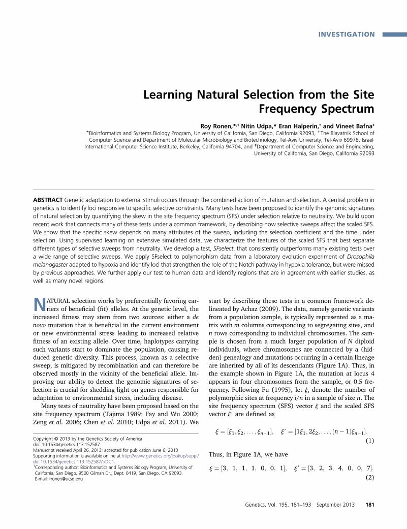
Figure 3 Power (5% FPR) of the SVMtest compared to other single-popula-tion tests of neutrality. Shown for 200data sets representing selective sweepswith selective coefficients s 2 [0.01,0.08], sampled at t 2 [0, 4000] gener-ations under selection. SFselect-s (black)assumes knowledge of (t, s), while SFse-lect (blue) assumes no prior knowledgeof these parameters. Time is shown ingenerations (bottom axes), and ln(2Ns)/sgenerations (top axes). Dotted verticallines show the mean time to fixation ofthe beneficial allele, which occurs at � 5ln(2Ns)/s generations.

184 R. Ronen et al.

and OmegaPlus (Alachiotis et al. 2012)). We compared ourcross-population SVMs to XP-CLR (Chen et al. 2010), XP-EHH (Sabeti et al. 2007), and Fst (Hudson et al. 1992).

We make a number of observations: (i) power changesproportionately to s for all tests, (ii) time to fixation of thebeneficial allele scales as ln(2Ns)/s (Campbell 2007), and(iii) all tests reach peak power following fixation and decayin the prefixation and postfixation regimes. We also notethat Tajima’s D performs better prefixation, due to the neg-ative weights (expected inflation) assigned to low frequen-cies and the positive weights (expected depletion) assignedto intermediate frequencies (Figure 2), while Fay andWu’s H performs better postfixation, due to the relativelyhigh weights assigned to low- and intermediate-frequencyvariants.

Invariably, our parameter-specific SVMs (SFselect-s) ex-hibit higher power compared to the other tests across thewide range of (s) and (t) combinations considered, remain-ing powerful throughout much of the postfixation regime.For example, at s = 0.08 the SVM shows 87% power after2000 generations, vs. 42% for the next best method. Like-wise, at s = 0.02, we see 85% power for the SVM at gener-ation 1000 vs. 57% for the next best method. These resultsdemonstrate the potential of statistical learning of weightfunctions for the scaled SFS. We next consider several mod-els of the scaled SFS learned by our parameter-specificSVMs.

Comparison with existing weighted linear combinations

We consider the feature weights learned by several of ourparameter-specific SVMs, compared with weight functionsof existing tests. Tajima’s D and Fay and Wu’s H (amongother tests) apply a weighted linear combination to the scaledSFS and are thus conceptually similar to trained (linear)SVMs. Differently put, both types of test represent linearmodels of the scaled SFS under nonneutral evolution.

For several reasons, only qualitative comparisons canbe made. First, we use a rescaled and binned version of theSFS. Unlike existing scaled SFS tests (such as D and H)that consider all allele frequencies between 1 and n 2 1,where n is the sample size, we rescale sample frequenciesto (0, 1] and bin them into n = 10 frequency bins (seeMethods). Second, while tests based on estimators of u

consider frequencies up to n 2 1, we extend the scaledSFS with an additional bin representing fixed differences

(see Methods). Finally, the rescaled, binned, and extendedscaled SFS vectors are normalized prior to learning andclassification. Hence, although absolute values of the learnedweights cannot be directly compared, we nevertheless gaininsight from a qualitative comparison with existing scaledSFS tests.

In Figure 4 we consider models learned by our specificSVMs (SFselect-s) from data sets simulated under relativelystrong selection (s = 0.04), sampled at times where D or Hshow high sensitivity. We consider differences and similari-ties between these models and the weighted linear combi-nations applied by D and H (Figure 2). For D, peak poweroccurs near the mean time of fixation (e.g., t = 700 gener-ations). We observe that the weights learned from this dataset do indeed bear some resemblance to those of Tajima’s D.Both have moderately positive weights in the intermediatefrequency range, which gradually decay toward the higherand lower frequencies (Figures 4A and 2A). However, themodels differ in their weight of the lowest frequency bin,which is highly negative in Tajima’s D.

At t = 2000 generations, H shows higher sensitivity com-pared to D. This is because unlike Tajima’s D, Fay and Wu’sH does not consider an inflation of low-frequency alleles asindicative of nonneutral evolution (Figure 2B). This helpsbecause after fixation, lower-frequency alleles are first to berestored to neutral levels via de novo mutation. In contrast,the weights learned from this data set are quite differentfrom those of H (Figures 4B and 2B), which was designedto capture an excess in high-frequency alleles (Fay and Wu2000). Specifically, we see positive linearly increasingweights toward the higher frequencies. This is effective be-cause de novo mutation takes longer to drift to higherfrequencies.

As stated previously, our fixed differences bin (rightmost)has no equivalent in Tajima’s D or Fay and Wu’s H. It is neg-atively weighted in both models shown because the beneficialallele (as well as hitchhiking alleles) has fixed, leading to manydifferentially fixed variants.

Comparison with previous learning-based methods

We further compared our results with two recent tests basedon supervised learning of summary statistics. The first, byPavlidis et al. (2010), applies SVMs to values of two tests:the v-statistic (Kim and Nielsen 2004), which is based on LDinformation, and the SweepFinder L-statistic (Nielsen et al.

Figure 4 Feature weights learned byparameter-specific SVMs. (A) Featureweights of the SVM trained on (s =0.04, t = 700), a regime in which Taji-ma’s D is sensitive. (B) Feature weightsof the SVM trained on (s = 0.04, t =2000), a regime in which Fay and Wu’sH is sensitive. We note that the right-most feature (representing fixed differ-ences) has no equivalent in D or H.

Learning Selection from the SFS 185

2005), which is based on the SFS. Additionally, the correla-tion between the genomic positions yielding maximal valuesof these tests is also used as a feature for learning. We usedimproved implementations of these algorithms, namely SweeD(P. Pavlidis, personal communication) for SweepFinder andOmegaPlus (Alachiotis et al. 2012) for the v-statistic. Thesecond approach we compare to, by Lin et al. (2011), appliesboosting to weak logistic regression classifiers learned fromLD- and SFS-based summary statistics computed within a re-gion. Namely, up (Tajima 1989), uH (Fay and Wu 2000), uW(Watterson 1975), Tajima’s D (Tajima 1989), Fay and Wu’sH (Fay and Wu 2000), and iHH (Sabeti et al. 2002).

In Figure 5 we show the power of SFselect-s compared toPavlidis et al. (2010) and Lin et al. (2011) under differentsweep parameters. Both SFselect-s and Lin et al. (2011) showhigher power compared to Pavlidis et al. (2010) across thesweep types considered. In addition, we observe that overallSFselect-s and Lin et al. (2011) show similar power, apartfrom a slight advantage to Lin et al. (2011) in a number oftime points under weaker selection (s = 0.01, 0.02).

We note that our feature set bears some conceptualsimilarity to that of Lin et al. (2011). With the exception ofthe iHH features, Lin et al. (2011) effectively learn from a smallset of weighted linear combinations of the scaled SFS. Ourframework demonstrates that similar power can be achievedby learning directly from the scaled SFS. In fact, our analysisshows that the small difference in observed power is explainedby the iHH features (Figure S4). Furthermore, the fundamentalnature of our feature set enables our framework to potentiallylearn linear combinations that are not captured by the set usedin Lin et al. (2011). In addition, we emphasize that althoughSFselect-s and Lin et al. (2011) show similar power in theparameter-specific case, in practice the parameters of a selectivesweep are seldom known. Next, we develop a generalized test

that can be applied without a priori knowledge of theseparameters.

Generalized SVM test (SFselect)

Learning-based approaches, by definition, require trainingdata. In the context of selection, this typically impliessimulating populations undergoing a selective sweep. Asa result, the parameters used in the simulation process areinevitably reflected in the trained models. Previous imple-mentations of learning-based approaches have been gearedtoward specific sweep parameters (Pavlidis et al. 2010; Linet al. 2011; as well as SFselect-s). Although we are able tolearn powerful models (and thus, tests) using this framework,such models are difficult to apply in practice. This is becausein most cases, the parameters (s, t) of a sweep are unknown.

To develop a test that performs well in practice, we musteither estimate these parameters or design a test that isrobust to them. As a first step, we compare the featureweights learned by parameter-specific SVMs across differentvalues of (s, t). In Figure 6, we show the cosine distancebetween all (�20,000) pairs (wi, wj), defined as

Dcos�wi;wj

�¼12wi �wj

jjwijj2  ����wj

����2

: (9)

Remarkably, we see two strong similarity blocks across allselection coefficients, partitioned roughly at the time offixation: a near-fixation similarity block encompassing timepoints close to (before and including) fixation of the bene-ficial allele, and a post-fixation similarity block encompassingthe later time points. Importantly, the similarity is transitiveacross selection coefficients, meaning that trained SVMs ina given block are similar not only to each other, but also toSVMs in corresponding blocks of other selection coefficients.For instance, members of the near-fixation block in s = 0.01

Figure 5 Power (0.05 FPR) of SFselect-scompared to tests based on supervisedlearning of summary statistics. We com-pare to Pavlidis et al. (2010) and Linet al. (2011). Shown for 200 data setsrepresenting selective sweeps with se-lective coefficients s 2 [0.01, 0.08], sam-pled at t 2 [0, 4000] generations underselection. Time shown in generations(bottom axes), and ln(2Ns)/s generations(top axes). The dashed vertical lines(gray) show the mean time to fixationof the beneficial allele, which occurs at�5 ln(2Ns)/s generations.

186 R. Ronen et al.

(spanning times t 2 [700, 1800]) show high similarity tomembers of the near-fixation block of s = 0.04 (spanningtimes t 2 [200, 500]). In the weaker selective pressures(s = 0.005,0.01), transitions between the two regimes are notas stark, due to the increased variance in fixation times (Durrett2002). This pairwise similarity structure is generally maintainedin cross-population SVMs as well (Figure S2).

Based on these findings, we retrained exactly two regime-specific SVMs denoted wnear and wpost. We trained theseSVMs on data corresponding to the observed similarityblocks, aggregated over the relevant time points of selectioncoefficients s 2 [0.02, 0.08]. For a given point j9, we use theestimated class probabilities from these SVMs to define ourtest score simply as

Sðj9Þ¼ max�Prðj9jw nearÞ; Pr

�j9jwpost

��: (10)

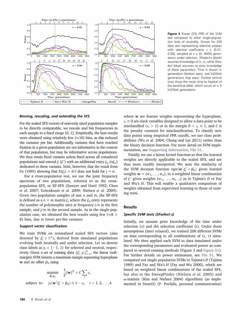
In Figure 7 we show the feature weights learned by thesegeneral SVMs (see Figure S3 for feature weights of the cor-responding cross-population SVMs). As expected when re-quiring less knowledge apriori, the general two-stage SVMhas less power to detect selective sweeps compared to theparameter-specific SVMs. Nevertheless, it dominates overexisting methods across much of the (s, t) parameter space(Figure 3), most notably so in the time points following fixa-tion of the beneficial allele. In certain regimes, D or H performsimilarly to our general model. This is in part because thefeature weights are somewhat similar. Particularly, we notethe similarity between the near-fixation SVM weights and D(Figure 2). For a corresponding analysis of power of the gen-eral cross-population SVM test (XP-SFselect), see Figure S1.

Finally, the class probabilities returned from wnear andwpost also carry information on whether a given data pointis in the prefixation or postfixation regime. By simply con-sidering the maximum of the two values, we were able toinfer the regime with .70% accuracy across times and se-lection pressures, excluding only those surrounding regimetransitions, which are inherently unclear (Figure 7C).

Fly models of hypoxia adaptation

We applied XP-SFselect to polymorphism frequency datafrom pooled whole-genome sequencing of D. melanogaster(Zhou et al. 2011). In this study, fly populations evolved formany generations (�200) in increasing levels of hypoxia(eventually reaching 4% O2), while genetically similar con-trols were kept in room air (21% O2) for cross-populationanalysis. The hypoxic stress was so strong that no wild-typefly survives in the final stage. Consequently, for a subset ofadaptive variants needed to survive under such conditions,the population under selection had likely reached a postfix-ation regime. At the same time, selective sweeps may beongoing for other variants. In that study, we used a log-ratiostatistic (Sf) that applies fixed weights to the scaled SFS andis sensitive to postfixation signal (Udpa et al. 2011).

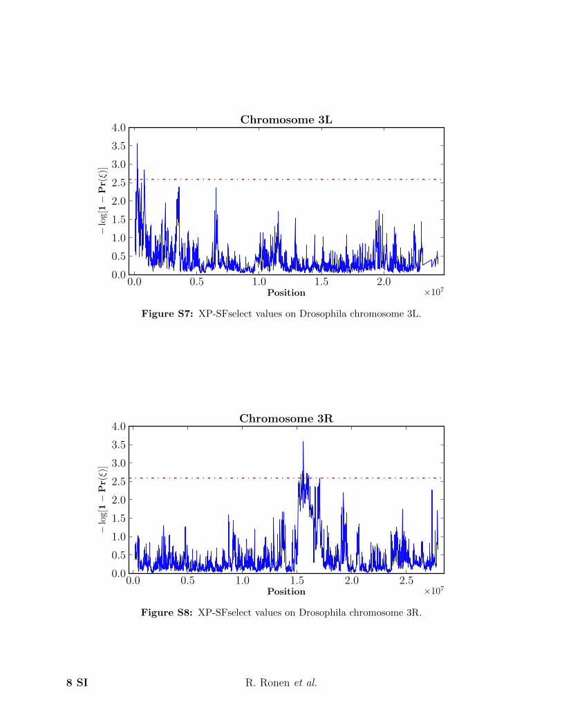
Applying a 1% genomic control FDR (see, for instance,Chen et al. 2010) in overlapping windows, and collapsingsignificant windows within 100 kbp of each other, we found17 significant regions using Sf. At the same time, XP-SFselectidentified 25 significant regions (Table S1, Figure S5, FigureS6, Figure S7, and Figure S8) including 11/17 (65%) of theSf regions. Many of the strongest candidates identified in

Figure 6 Pairwise cosine distance between 200trained SVMs. SVMs were trained on data sim-ulated under different selection pressures s 2[0.01, 0.08], sampled at different times underselection t 2 [0, 4000] generations. Boundariesbetween selection pressures are denoted byblack lines and mean times to fixation by bluedashed lines. We observe two similarity blocksat each selection pressure, corresponding to“near fixation”and “postfixation” of the bene-ficial allele. The stronger the selection (e.g., bot-tom right) the earlier/shorter the near-fixationstage, and vice versa.

Learning Selection from the SFS 187

Zhou et al. (2011), including HDAC4 and hang, were alsofound by XP-SFselect. In addition, XP-SFselect identified 14unique regions as significant. For a breakdown of significantwindows by regime, see Table 1.

There is some evidence that XP-SFselect is more robustthan Sf. For instance, one region deemed significant by Sf,but not XP-SFselect, appears to be an artifact. This region(chrX:14.61–14.85 Mb) is significant under Sf due to littlehaplotype diversity in the adapted population, caused bya large block of fixed SNPs. Importantly, the control popu-lation also shows reduced diversity in this region, with thesame block present at �80% frequency. This is likely theresult of an event prior to population divergence and, thus,not caused by the hypoxic stress. Sf correctly identified lowdiversity in the adapted population, but weighed the high-frequency (nonfixed) alleles in controls as evidence ofincreased diversity instead (Udpa et al. 2011). In contrast,XP-SFselect correctly identifies the frequency difference of20% as uninteresting genome wide.

XP-SFselect may also be more sensitive. The main conclu-sion of Zhou et al. (2011) was that the Notch pathway isgenetically involved in hypoxia tolerance, based on the pres-ence of two Notch inhibitory genes (HDAC4 and Hairless) insignificant regions. We confirmed these with XP-SFselect butalso identified another significant region (chrX:2.87–3.44Mb) containing a third component of the Notch pathway—the Notch gene itself (Figure 8). Upon further inspection, theNotch gene shows an interesting profile. We see very littlediversity in the adapted population (mean coding SNP fre-quency, 0.99), while corresponding control frequencies arelow (mean, 0.26). These include a nonsynonymous SNP(S29P) fixed in the adapted population and completely ab-sent in controls. This serine is located in the N-terminal signalpeptide, important for moving Notch to the membrane, whereactivation can occur. A key feature of the signal peptide is a longstretch of hydrophobic residues that stabilize by forming a he-lical structure. The serine at position 29 is in the middle of thisstretch, and is hydrophilic, potentially impairing the ability ofthe signal peptide to form the helix. Replacing the serine witha hydrophobic proline may increase the stability (and thus

efficiency) of the signal peptide in guiding Notch to themembrane.

Models of human demography

To assess the ability of our framework to detect selection undercomplex demographic scenarios, as in many extant humanpopulations, we simulated data under a more involved model.A strength of our framework is that if the demographic historyis well characterized, a specific model of the SFS that is fine-tuned to that history can be learned. Focusing on the recentdemographic histories of Northern Europeans and WesternAfricans, we note that multiple models can potentially explainthe observed patterns of polymorphism (Schaffner et al. 2005;Voight et al. 2005; Fagundes et al. 2007) and that a clearconsensus has not yet been reached.

We use a model described recently by Gravel et al. (2011),with two instantaneous bottlenecks followed by a period ofexponential growth in the European population (Figure 9). Inthis demographic scenario, we simulated a beneficial (s =0.02, 0.005) allele in the European population, introducedat various time points [20, 25, and 50 thousand years ago(kya)]. In our simulations, we assume neutral evolution priorto the populations separating. As a result, we do not expectcross-population tests to have a distinct advantage, as theirmain strength is to decrease the effect of shared selection inthe ancestral population.

We evaluated the power of single- and cross-populationSVMs trained on the simulated data to detect selection.Table 2 shows power of the SVMs at various time points,

Table 1 Regime of selection as determined by SVM

Near-fixationregime

Postfixationregime

XP-SFselect and Sf windows 75 274XP-SFselect-only windows 211 8

The number of genomic windows found significant under XP-SFselect (568 overall)with higher class probabilities for the near-fixation, or the post-fixation regime.Showing windows found only by XP-SFselect, as well those identified by both XP-SFselect and Sf. These results imply that while Sf is sensitive to the post-fixationregime, XP-SFselect captures both types of selection.

Figure 7 Feature weights of the twogeneralized regime SVMs and regimeinference rates. (A) Weights learned bythe near-fixation SVM. (B) Weightslearned by the postfixation SVM. Minorallele frequencies were distributed ton = 11 bins, with the last bin dedicatedto fixed differences. (C) Fraction of truepositives with postfixation class proba-bility greater than that of near fixation,as function of time. Due to lower absolutenumber of true positives in the weakerselection pressures (s = 0.01, 0.02), weobserve increased variance. The shadedregion surrounding 4ln(2Ns)/s generationscontains the mean times to fixation of thebeneficial alleles.

188 R. Ronen et al.

compared with other tests. As in constant-sized populations,we observe that Fay and Wu’s H is less powerful except inthe late stages (e.g., 50 kya for s= 0.02) and that among thecross-population tests, XP-CLR is generally more powerfulthan XP-EHH. Additionally, we note that both the single- andcross-population SVMs show significantly higher power than allother tests. Finally, as postulated, we did not observe a consistentadvantage for cross-population over single-population tests.

Application to human populations

As no clear consensus exists on the demographic history ofany human population, we applied our general SVM test(XP-SFselect) to data from two human populations se-quenced by the 1000 Genomes Project (Abecasis et al.2010): individuals of Northern European descent from Utah(CEU, 88 individuals) and Yoruban individuals from Nigeria(YRI, 85 individuals). These populations have been consid-ered in several studies of selection (Frazer et al. 2007; Sabetiet al. 2007; Pickrell et al. 2009; Chen et al. 2010); thus weexpected our results to overlap with previously reportedregions. Using a 0.2% genomic control FDR in overlappingwindows, and collapsing significant windows within 100kbp of each other, we identified 339 distinct regions, ofwhich 217 overlap known genes. As expected, several ofthe regions we find have been previously reported. We do,however, find signal in regions that have not so far beenreported and may be of phenotypic interest. In Table S2,we list 40 regions showing the strongest signal of selectivesweep using XP-SFselect. We used SnpEff (Cingolani et al.2012) to annotate the functional impact of mutations and

extracted all high-impact (splice or nonsense) mutations aswell as all nonsynonymous mutations deemed damaging bySIFT (Kumar et al. 2009). In Table S3 we list the subset ofthese SNPs that fall within significant regions and showa high-frequency differential ($30%) between the two pop-ulations (we find 11 such SNPs genome wide).

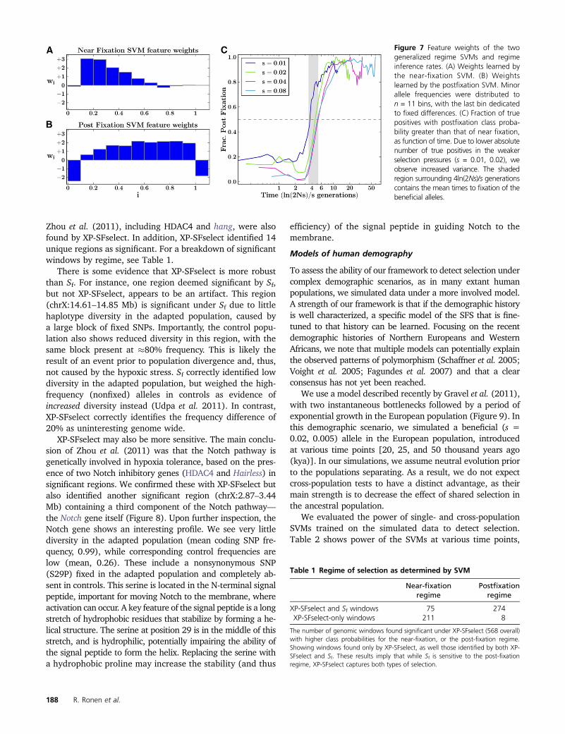
Known regions identified by XP-SFselect: We compared thesignificant regions found by XP-SFselect to the top regionsidentified in four previous studies of the same populations:Chen et al. (2010), Pickrell et al. (2009), Frazer et al. (2007),and Sabeti et al. (2007). Of the 339 regions, 36 were reportedin these studies (8 of top 40). This partial overlap likely stemsfrom the considerable difference in density between the gen-otyping data used in the previous studies and that of whole-genome sequencing. When considering the top 1% of ourresults, however, the overlap becomes substantial (see Figure10). Specifically, the overlap was 35.3% for Frazer et al.(2007), 47.8% for Pickrell et al. (2009), 57.9% for Sabetiet al. (2007), and 67.5% for Chen et al. (2010).

Of the previously reported regions, particularly noteworthyare the genomic regions of KITLG (12q21.32) and SLC24A5(15q21.1), found at 0.002 and 0.1% of the genome widedistribution, respectively. Variation in these genes has beenassociated with skin pigmentation and was reported to showevidence of selection (Pickrell et al. 2009). Additionally, wefound the region containing the lactase gene (LCT) significantat 0.16% genome wide. Several studies have reported thisgene as showing evidence of selection in Northern Europeanpopulations (Bersaglieri et al. 2004; Chen et al. 2010).

Figure 8 Signatures of selective sweeps affect-ing Notch pathway in hypoxia tolerant flies. XP-SFselect and Sf on fly chromosome X. Theregions highlighted in gray were found signifi-cant by both Sf and XP-SFselect. The regionhighlighted in yellow is an artifactual regiondeemed significant under Sf, but not underXP-SFselect. The region highlighted in greencontains the Notch gene, which activates theNotch signaling pathway. The mutation S29Pmay enhance the activity of Notch by improvingthe stability of the signal peptide domain. Theregion highlighted in red contains the HDAC4gene, including the mutation A1009S near theactive site of the protein, which may reduce itsability to affect Notch gene targets. Both ofthese mutations are consistent with hypoxia-tolerant flies genetically activating the Notchpathway as a mechanism of adaptation.

Learning Selection from the SFS 189

Novel regions identified by XP-SFselect: We identified aregion (1q44) significant at 0.01% genome wide, containinga cluster of olfactory receptor (OR) genes: OR2T8, OR2L13,OR2L8, OR2AK2, and OR2L1P. Notably, the subregion con-taining OR2L8, OR2L13, and OR2AK2 has particularly lowdiversity in Northern Europeans, with a dense block of 97nearly fixed SNPs (mean frequency, 0.95) in comparison to thesame block in Western Africans (mean frequency, 0.24). Thisblock also includes six nonsynonymous SNPs, of which twowere deemed damaging (rs10888281 and rs4478844; seeTable S3). Olfactory receptors make up the largest gene fam-ily, containing several hundreds of genes, many of which arepseudogenes. It has been suggested that a subset of (intact)OR genes are subject to selection in several human popula-tions (Gilad et al. 2003; Pickrell et al. 2009), but to the bestof our knowledge this OR cluster has not been identified asunder selection in Northern European or Western Africanpopulations.

Additionally, the regions containing MSR1 (macrophagescavenger receptor 1) and MASP2 (mannan-binding lectinserine protease 2) were found significant at 0.07% and0.09% of the genome wide distribution, respectively. Thesegenes also contained 2 of the 11 variants with high-frequency differential between the populations that weredeemed damaging (rs435815 and rs12711521; see TableS3). Interestingly, the ortholog of MSR1 has been shownto confer a protective effect from malaria infection in a re-cent study on mice (Rosanas-Urgell et al. 2012). At the sametime, it has been shown to have a strong signal of balancingselection in African primate populations (Tung et al. 2009).Likewise, MASP2 has been associated with immune re-sponse to several diseases, including Chagas disease (Boldtet al. 2011), hepatitis C (Tulio et al. 2011), and placentalmalaria (Holmberg et al. 2012). Mutations in this gene

(including rs12711521 (Boldt et al. 2011), see Table S3)have been linked to both the activity (Thiel et al. 2009)and expression levels (Thiel et al. 2007) of the protein. Sucha sharp signal at these loci may imply a differential diseaselandscape between the two populations. For instance, it isconceivable that the YRI population has had to adapt atthese loci to deal effectively with malaria, whereas CEUindividuals have not had this stress.

Computational considerations

Our approach is composed of three main steps: data simula-tion, model training, and region classification. The first step,simulation, is performed with external tools and is thereforeoutside the scope of this article. For training and classification,there are two options. One may use our pretrained generalmodel for classifying genomic regions as selected or neutral.This approach is very fast: a complete cross-population scan ofthe human genome (of the CEU and YRI populations)completed in under 2 hr on a standard desktop with 4 GBRAM. We note that this was done on whole-genome sequenc-ing data, with considerably more variants than genotyping.

Another option is to train on data simulated under a specificmodel (e.g., given a known demographic scenario). The com-putational space and time required for training strongly de-pend on the size of the training data. In our experience,training a specific model (�1000 training examples) requiredunder 1 min, while training the general model (�90,000 train-ing examples) required close to 2 hr.

It should also be noted that training can potentially befaster. We used the LIBSVM implementation (Graf et al. 2003;Chang and Lin 2011; Pedregosa et al. 2011) due to its capa-bility to calculate class probabilities, which enabled bettercontrol of FPR. A strictly linear SVM implementation, suchas the one used by LIBLINEAR (Fan et al. 2008), will yieldmuch better scaling of training times.

Discussion

The site frequency spectrum is heavily skewed underpositive selection. Using supervised learning, we sought todevelop a test that would yield not only improved power todetect a sweep, but also insight into the behavior of the SFS

Table 2 Power (0.05 FPR) of different tests on data simulatedunder a demographic model

s kya D H XP-CLR XP-EHH SFselect-s XP-SFselect-s

20 0.64 0.05 0.58 0.22 0.85 0.800.02 25 0.82 0.22 0.77 0.28 0.89 0.88

50 0.97 0.95 0.99 0.40 0.99 0.99

20 0.04 0.04 0.06 0.06 0.29 0.400.005 25 0.05 0.03 0.04 0.05 0.23 0.48

50 0.45 0.11 0.41 0.25 0.71 0.66

The beneficial allele was simulated in the Northern European population (CEU),while the Western African population (YRI) evolved neutrally and was used ascontrol for the cross-population tests.

Figure 9 The demographic model used to simulate the CEU and YRIpopulations. The model is shown with time flowing downward. Modelparameters are as described by Gravel et al. (2011), including a growthrate of 0.48% per generation in the European expansion period. Wesimulated an allele under positive selection (s = 0.02, 0.005) introduced20, 25, and 50 kya (assuming 25 years per generation).

190 R. Ronen et al.

under various sweep types. The scaled SFS, being uniform inexpectation under neutrality, provided a natural choice offeatures to learn from. Rather than a fixed weight functionthat performs well only under certain regimes, we were ableto learn multiple weight functions of the scaled SFS, eachproviding optimal performance in its respective regime. Whencombined, these resulted in a usable test that improves overexisting methods for both simulated and real data.

Although SVMs are standard practice in supervisedlearning, other classification methods are also applicable.A popular alternative is logistic regression, with optional (L1

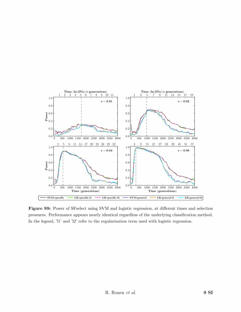
or L2 norm) regularization of the model. While logistic re-gression has the advantage of providing a naturally contin-uous output, it proved less effective for our purposes. Thetwo methods performed similarly in the single-populationtest, but we observed a noticeable decrease in power ofthe cross-population test (Figure S9 and Figure S10). Thisis likely due to the difference in loss function. While SVMsuse a one-sided hinge loss, with no penalty for well-classifiedpoints outside the classification margin, logistic regressionminimizes the log loss. Here, correctly classified points—including those outside the SVM margin—incur a (small)penalty. This may have a significant impact if the data aredense near the margins, which is likely the case for the XP-SFS vectors.

Given prior information on a population’s history andmode of selection, one may wish to apply weights to theregime SVMs, thereby increasing the sensitivity of the test.

In our fly data, we can safely assume a postfixation regimefor those loci most (and earliest) affected by selection, dueto the high selective stress and relatively long time (�200generations). Thus, we can increase the sensitivity in thoseregions by weighting down the probabilities returned fromthe near-fixation SVM. Of course, this will decrease the sen-sitivity for regions in near-fixation regime. When applyingno such bias to the regime of selection, our results indicatethat SFselect can identify both types of selection, while pre-vious methods were limited to specific regimes (Table 1).

Finally, although SFselect has high power in the near-fixation and postfixation regimes, there may be room forimprovement in early selection. We note that tests based onhaplotype diversity, such as iHH (Sabeti et al. 2002), areconsidered advantageous in this regime. To increase sensi-tivity in this regime, one might incorporate frequencies ofdominant haplotypes as additional features. Moreover, al-though here we considered only the hard sweep model ofpositive selection, one might use a similar framework to in-vestigate more complex scenarios, including the soft sweepmodel. Our results suggest that applying statistical learningdirectly to the scaled SFS can provide valuable insights fordetecting nonneutral evolutionary processes.

Acknowledgments

We thank Efrat Golan for technical assistance, as well as YanivErlich, Matan Hofree, Boyko Kakaradov, and two anonymous

Figure 10 Cumulative rank distribution of the topregions reported by previous studies, in the results ofXP-SFselect. Rank distributions of previous studies areshown in red and those of 1000 identically sized sets ofregions (per study) sampled at random from the ge-nome are shown in blue. We see a significant enrich-ment of the regions from previous studies among thetop 0.2% (dark shading) and 1% (light shading) of XP-SFselect results. The P-values shown are for a Mann–Whitney U-test with null hypothesis of equality be-tween the rank distribution of a given study and thatof the corresponding random samples. The studiescompared to were: Chen et al. (2010), Pickrell et al.(2009), Sabeti et al. (2007), and Frazer et al. (2007).

Learning Selection from the SFS 191

reviewers for valuable suggestions. We also thank NoahRosenberg for comments on the manuscript and PavlosPavlidis for sharing instructions and code of OmegaPlusand SweeD. R.R. and N.U. were supported by NationalScience Foundation (NSF) grant CCF-1115206. E.H. is afaculty fellow of the Edmond J. Safra Program at Tel AvivUniversity and was supported in part by the German IsraeliFoundation (grant 0603806851). V.B. was supported byNational Institutes of Health (NIH) grant 5RO1-HG004962.

Literature Cited

Abecasis, G. R., D. Altshuler, A. Auton, L. D. Brooks, R. M. Durbinet al., 2010 A map of human genome variation from popula-tion-scale sequencing. Nature 467: 1061–1073.

Achaz, G., 2009 Frequency spectrum neutrality tests: one for alland all for one. Genetics 183: 249–258.

Alachiotis, N., A. Stamatakis, and P. Pavlidis, 2012 OmegaPlus:a scalable tool for rapid detection of selective sweeps in whole-genome datasets. Bioinformatics 28: 2274–2275.

Bersaglieri, T., P. C. Sabeti, N. Patterson, T. Vanderploeg, S. F.Schaffner et al., 2004 Genetic signatures of strong recent positiveselection at the lactase gene. Am. J. Hum. Genet. 74: 1111–1120.

Boldt, A. B., P. R. Luz, and I. J. Messias-Reason, 2011 MASP2haplotypes are associated with high risk of cardiomyopathy inchronic Chagas disease. Clin. Immunol. 140: 63–70.

Campbell, C. D., J. X. Chong, M. Malig, A. Ko, B. L. Dumont et al.,2012 Estimating the human mutation rate using autozygosityin a founder population. Nat. Genet. 44: 1277–1281.

Campbell, R., 2007 Coalescent size vs. coalescent time withstrong selection. Bull. Math. Biol. 69: 2249–2259.

Chang, C. C., and C. J. Lin, 2011 LIBSVM: a library for supportvector machines. ACM Trans. Intell. Syst. Technol. 2: 27:1–27:27.

Chen, H., R. E. Green, S. Paabo, and M. Slatkin, 2007 The jointallele-frequency spectrum in closely related species. Genetics177: 387–398.

Chen, H., N. Patterson, and D. Reich, 2010 Population differenti-ation as a test for selective sweeps. Genome Res. 20: 393–402.

Cingolani, P., A. Platts, M. Coon, T. Nguyen, L. Wang et al.,2012 A program for annotating and predicting the effects ofsingle nucleotide polymorphisms, SnpEff: SNPs in the genome ofDrosophila melanogaster strain w1118; iso-2; iso-3. Fly 6: 80–92.

Durrett, R., 2002 Probability Models for DNA Sequence Evolution,Ed. 2. Springer-Verlag, New York.

Fagundes, N. J. R., N. Ray, M. Beaumont, S. Neuenschwander, F. M.Salzano et al., 2007 Statistical evaluation of alternative models ofhuman evolution. Proc. Natl. Acad. Sci. USA 104: 17614–17619.

Fan, R.-E., K.-W. Chang, C.-J. Hsieh, X.-R. Wang, and C.-J. Lin,2008 LIBLINEAR: a library for large linear classification. J.Mach. Learn. Res. 9: 1871–1874.

Fay, J. C., and C. I. Wu, 2000 Hitchhiking under positive Darwinianselection. Genetics 155: 1405–1413.

Frazer, K. A., D. G. Ballinger, D. R. Cox, D. A. Hinds, L. L. Stuveet al., 2007 A second generation human haplotype map of over3.1 million SNPs. Nature 449: 851–861.

Fu, Y. X., 1995 Statistical properties of segregating sites. Theor.Popul. Biol. 48: 172–197.

Gilad, Y., C. D. Bustamante, D. Lancet, and S. Paabo, 2003 Naturalselection on the olfactory receptor gene family in humans andchimpanzees. Am. J. Hum. Genet. 73: 489–501.

Graf, A., A. Smola, and S. Borer, 2003 Classification in a normal-ized feature space using support vector machines. IEEE Trans.Neural Networks 14: 597–605.

Gravel, S., B. M. Henn, R. N. Gutenkunst, A. R. Indap, G. T. Marthet al., 2011 Demographic history and rare allele sharingamong human populations. Proc. Natl. Acad. Sci. USA 108:11983–11988.

Gutenkunst, R. N., R. D. Hernandez, S. H. Williamson, and C. D.Bustamante, 2009 Inferring the joint demographic history ofmultiple populations from multidimensional SNP frequencydata. PLoS Genet. 5: e1000695.

Holmberg, V., P. Onkamo, E. Lahtela, P. Lahermo, G. Bedu-Addoet al., 2012 Mutations of complement lectin pathway genesMBL2 and MASP2 associated with placental malaria. Malar. J.11: 61.

Hudson, R. R., 2002 Generating samples under a Wright–Fisherneutral model of genetic variation. Bioinformatics 18: 337–338.

Hudson, R. R., M. Slatkin, and W. P. Maddison, 1992 Estimationof levels of gene flow from DNA sequence data. Genetics 132:583–589.

Kim, Y., and R. Nielsen, 2004 Linkage disequilibrium as a signa-ture of selective sweeps. Genetics 167: 1513–1524.

Kingman, J. F. C., 1982 On the genealogy of large populations. J.Appl. Probab. 19: 27–43.

Kumar, P., S. Henikoff, and P. C. Ng, 2009 Predicting the effects ofcoding non-synonymous variants on protein function using theSIFT algorithm. Nat. Protoc. 4: 1073–1081.

Lin, K., H. Li, C. Schltterer, and A. Futschik, 2011 Distinguishingpositive selection from neutral evolution: boosting the perfor-mance of summary statistics. Genetics 187: 229–244.

Nachman, M. W., and S. L. Crowell, 2000 Estimate of the muta-tion rate per nucleotide in humans. Genetics 156: 297–304.

Nielsen, R., S. Williamson, Y. Kim, M. J. Hubisz, A. G. Clark et al.,2005 Genomic scans for selective sweeps using SNP data. Ge-nome Res. 15: 1566–1575.

Nielsen, R., M. J. Hubisz, I. Hellmann, D. Torgerson, A. M. Andreset al., 2009 Darwinian and demographic forces affecting hu-man protein coding genes. Genome Res. 19: 838–849.

Pavlidis, P., J. D. Jensen, and W. Stephan, 2010 Searching forfootprints of positive selection in whole-genome snp data fromnonequilibrium populations. Genetics 185: 907–922.

Pedregosa, F., G. Varoquaux, A. Gramfort, V. Michel, B. Thirionet al., 2011 Scikit-learn: machine learning in python. J. Mach.Learn. Res. 12: 2825–2830.

Pickrell, J. K., G. Coop, J. Novembre, S. Kudaravalli, J. Z. Li et al.,2009 Signals of recent positive selection in a worldwide sam-ple of human populations. Genome Res. 19: 826–837.

Rosanas-Urgell, A., L. Martin-Jaular, J. Ricarte-Filho, M. Ferrer, S.Kalko et al., 2012 Expression of non-TLR pattern recognitionreceptors in the spleen of BALB/c mice infected with Plasmo-dium yoelii and Plasmodium chabaudi chabaudi AS. Mem. Inst.Oswaldo Cruz 107: 410–415.

Sabeti, P. C., D. E. Reich, J. M. Higgins, H. Z. Levine, D. J. Richteret al., 2002 Detecting recent positive selection in the humangenome from haplotype structure. Nature 419: 832–837.

Sabeti, P. C., P. Varilly, B. Fry, J. Lohmueller, E. Hostetter et al.,2007 Genome-wide detection and characterization of positiveselection in human populations. Nature 449: 913–918.

Sawyer, S. A., and D. L. Hartl, 1992 Population genetics of poly-morphism and divergence. Genetics 132: 1161–1176.

Schaffner, S. F., C. Foo, S. Gabriel, D. Reich, M. J. Daly et al.,2005 Calibrating a coalescent simulation of human genomesequence variation. Genome Res. 15: 1576–1583.

Shriver, M. D., G. C. Kennedy, E. J. Parra, H. A. Lawson, V. Sonparet al., 2004 The genomic distribution of population substruc-ture in four populations using 8,525 autosomal SNPs. Hum.Genomics 1: 274–286.

Tajima, F., 1989 Statistical method for testing the neutral muta-tion hypothesis by DNA polymorphism. Genetics 123: 585–595.

192 R. Ronen et al.

Thiel, S., R. Steffensen, I. J. Christensen, W. K. Ip, Y. L. Lau et al.,2007 Deficiency of mannan-binding lectin associated serineprotease-2 due to missense polymorphisms. Genes Immun. 8:154–163.

Thiel, S., M. Kolev, S. Degn, R. Steffensen, A. G. Hansen et al.,2009 Polymorphisms in mannan-binding lectin (MBL)-associ-ated serine protease 2 affect stability, binding to MBL, and en-zymatic activity. J. Immunol. 182: 2939–2947.

Tulio, S., F. R. Faucz, R. I. Werneck, M. Olandoski, R. B. Alexandreet al., 2011 MASP2 gene polymorphism is associated with sus-ceptibility to hepatitis C virus infection. Hum. Immunol. 72:912–915.

Tung, J., A. Primus, A. J. Bouley, T. F. Severson, S. C. Alberts et al.,2009 Evolution of a malaria resistance gene in wild primates.Nature 460: 388–391.

Udpa, N., D. Zhou, G. G. Haddad, and V. Bafna, 2011 Tests ofselection in pooled case-control data: an empirical study. Front.Genet. 2: 83.

Voight, B. F., A. M. Adams, L. A. Frisse, Y. Qian, R. R. Hudson et al.,2005 Interrogating multiple aspects of variation in a full rese-quencing data set to infer human population size changes. Proc.Natl. Acad. Sci. USA 102: 18508–18513.

Watterson, G., 1975 On the number of segregating sites in genet-ical models without recombination. Theor. Popul. Biol. 7: 256–276.

Wu, T. F., C. J. Lin, and R. C. Weng, 2004 Probability estimatesfor multi-class classification by pairwise coupling. J. Mach.Learn. Res. 5: 975–1005.

Zeng, K., Y.-X. Fu, S. Shi, and C.-I. Wu, 2006 Statistical tests fordetecting positive selection by utilizing high-frequency variants.Genetics 174: 1431–1439.

Zhou, D., N. Udpa, M. Gersten, D. W. Visk, A. Bashir et al.,2011 Experimental selection of hypoxia-tolerant Drosophilamelanogaster. Proc. Natl. Acad. Sci. USA 108: 2349–2354.

Communicating editor: W. Stephan

Learning Selection from the SFS 193

GENETICSSupporting Information

http://www.genetics.org/lookup/suppl/doi:10.1534/genetics.113.152587/-/DC1

Learning Natural Selection from the SiteFrequency Spectrum

Roy Ronen, Nitin Udpa, Eran Halperin, and Vineet Bafna

Copyright © 2013 by the Genetics Society of AmericaDOI: 10.1534/genetics.113.152587

File S1

Supporting Information

Power and False Positive Rate. In order to evaluate the power of SFselect and XP-

SFselect to detect positive selection as compared to other neutrality tests, we applied these

tests to several datasets simulated under different model parameters. For a given test on

a given dataset, the power at 5% false positive rate (FPR) was estimated as the fraction

of test-statistic values exceeding a set threshold when applied to the selected samples. The

threshold was set to the top 5% of the null distribution, obtained by applying the test

to neutral samples. For cross-populations tests (including XP-SFselect) we used the same

procedure, only applying the test to selected vs. neutral samples, while the null was obtained

by applying the test to neutral1 vs. neutral2 samples.

SVM implementation details. We used a linear (dot product) kernel function SVM.

Linear kernels have two important advantages. First, because feature-weights learned by

a linear SVM represent a maximum-margin separating hyperplane of the training data in

the problem space (rather than in a higher dimensional space), they correspond to the

relative importance of features in separating the training data, making the trained SVM

easily interpretable. Secondly, normalization of the training and testing data is done in the

input space, without the need for complicated normalization of the kernel function itself

(Graf et al. 2003).

The SVM implementation we used was from the LIBSVM library (Chang and Lin 2011),

packaged in the python library scikit-learn (Pedregosa et al. 2011). For the parameter-specific

SVMs, where we lacked sufficient simulated data to hold the test data out of training, we

report power as the mean over 50-fold cross validation. For the general two-stage SVM

(SFselect and XP-SFselect), testing and training were done on completely separate datasets.

2 SI R. Ronen et al.

0 500 1000 1500 2000 2500 3000 3500 40000.0

0.2

0.4

0.6

0.8

1.0

Pow

er

s = 0.01

1 2 3 4 5 6 7 8 9 10 11Time (ln(2Ns)/s generations)

0 500 1000 1500 2000 2500 3000 3500 40000.0

0.2

0.4

0.6

0.8

1.0s = 0.02

1 3 5 7 9 11 13 15 17 19Time (ln(2Ns)/s generations)

0 500 1000 1500 2000 2500 3000 3500 4000Time (generations)

0.0

0.2

0.4

0.6

0.8

1.0

Pow

er

s = 0.04

2 5 8 11 14 17 20 23 26 29 32

0 500 1000 1500 2000 2500 3000 3500 4000Time (generations)

0.0

0.2

0.4

0.6

0.8

1.0s = 0.08

3 9 15 21 27 33 39 45 51 57

XP-CLR XP-EHH Fst XP-SFselect-s XP-SFselect

Figure S1: Power (0.05 FPR) of the cross-population SVM test compared to other cross-

population tests of neutrality. Shown across selection pressures s∈ [0.01, 0.08] and times τ ∈ [0, 4000].

The (black) line labelled ‘XP-SFselect-s’ shows power when assuming knowledge of the selection

coefficient and the time (τ and s, respectively). The (blue) line labeled ‘XP-SFselect’ shows power

when no prior knowledge of (s, τ) is assumed. Time is shown in generations (bottom axes), and

ln(2Ns)/s generations (top axes). The dashed vertical lines (grey) show the mean time to fixation

of the beneficial allele, which occurs at ≈ 5 ln(2Ns)/s generations.

R. Ronen et al. 3 SI

Figure S2: Pairwise cosine distance between 200 SVMs trained on cross-population data (matrices

of the XP-SFS scaled to 8 × 8 frequency bins, and vectorized). The data was simulated under

different selection pressures s ∈ [0.005, 0.08], and sampled at different times under selection τ ∈[0, 4000] generations. Selection pressure boundaries are denoted by black lines, and mean time to

fixation for each pressure is denoted by dashed blue lines. We observe two main similarity blocks at

each selection pressure, corresponding to ”near fixation” and ”post-fixation” of the beneficial allele.

The stronger the selection pressure (e.g., bottom right) the earlier and shorter the near-fixation

stage, and vice versa.

4 SI R. Ronen et al.

1/7 2/7 3/7 4/7 5/7 6/7 7/7

Case Freq.

1/7

2/7

3/7

4/7

5/7

6/7

7/7

Contr

ol

Fre

q.

Near-Fixation feature weights

1/7 2/7 3/7 4/7 5/7 6/7 7/7

Case Freq.

1/7

2/7

3/7

4/7

5/7

6/7

7/7

Post-Fixation feature weights

1/7 2/7 3/7 4/7 5/7 6/7 7/7

−5

0

5

10

Column Sums

1/7 2/7 3/7 4/7 5/7 6/7 7/7

−5

0

5

10

Column Sums

−3.0−2.5−2.0−1.5−1.0−0.5+0.0+0.5+1.0+1.5+2.0+2.5+3.0+3.5+4.0

Figure S3: Feature weights learned from the XP-SFS on data corresponding to the two observed

regimes of selection: (A) near-fixation, and (B) post-fixation. Minor allele frequencies were dis-

tributed to 8× 8 bins, where the rightmost column (top row) was dedicated to alleles fixed in the

selected (neutral) population. Decision function constants were β0=−0.80, and β0=−0.56 for the

near-fixation, and post-fixation SVMs, respectively.

R. Ronen et al. 5 SI

0 500 1000 1500 2000 2500 3000 3500 40000.0

0.2

0.4

0.6

0.8

1.0

Pow

er

s = 0.01

1 2 3 4 5 6 7 8 9 10 11Time (ln(2Ns)/s generations)

0 500 1000 1500 2000 2500 3000 3500 40000.0

0.2

0.4

0.6

0.8

1.0s = 0.02

1 3 5 7 9 11 13 15 17 19Time (ln(2Ns)/s generations)

0 500 1000 1500 2000 2500 3000 3500 4000Time (generations)

0.0

0.2

0.4

0.6

0.8

1.0

Pow

er

s = 0.04

2 5 8 11 14 17 20 23 26 29 32

0 500 1000 1500 2000 2500 3000 3500 4000Time (generations)

0.0

0.2

0.4

0.6

0.8

1.0s = 0.08

3 9 15 21 27 33 39 45 51 57

SFselect-s SFselect-s-iHH Lin et al. Pavlidis et al.

Figure S4: Power (0.05 FPR) of neutrality tests based on supervised learning. The line

labelled ‘SFselect-s’ shows power of the regular parameter-specific SVMs, while the line labelled

‘SFselect-s-iHH’ shows power when including the iHH features described in Lin et al. (2011). Shown

for selection pressures s ∈ [0.01, 0.08] and times τ ∈ [0, 4000], with time in generations (bottom

axes), and ln(2Ns)/s generations (top axes). The dashed vertical lines (grey) show the mean time

to fixation of the beneficial allele, which occurs at ≈ 5 ln(2Ns)/s generations.

6 SI R. Ronen et al.

0.0 0.5 1.0 1.5 2.0Position ×107

0.0

0.5

1.0

1.5

2.0

2.5

3.0

3.5−

log[1−

Pr(ξ)

]

Chromosome 2L

Figure S5: XP-SFselect values on Drosophila chromosome 2L.

0.0 0.5 1.0 1.5 2.0Position ×107

0.0

0.5

1.0

1.5

2.0

2.5

3.0

3.5

4.0

4.5

−lo

g[1−

Pr(ξ)

]

Chromosome 2R

Figure S6: XP-SFselect values on Drosophila chromosome 2R.

R. Ronen et al. 7 SI

0.0 0.5 1.0 1.5 2.0Position ×107

0.0

0.5

1.0

1.5

2.0

2.5

3.0

3.5

4.0

−lo

g[1−

Pr(ξ)

]

Chromosome 3L

Figure S7: XP-SFselect values on Drosophila chromosome 3L.

0.0 0.5 1.0 1.5 2.0 2.5Position ×107

0.0

0.5

1.0

1.5

2.0

2.5

3.0

3.5

4.0

−lo

g[1−

Pr(ξ)

]

Chromosome 3R

Figure S8: XP-SFselect values on Drosophila chromosome 3R.

8 SI R. Ronen et al.

0 500 1000 1500 2000 2500 3000 3500 40000.0

0.2

0.4

0.6

0.8

1.0

Pow

er

s = 0.01

1 2 3 4 5 6 7 8 9 10 11Time (ln(2Ns)/s generations)

0 500 1000 1500 2000 2500 3000 3500 40000.0

0.2

0.4

0.6

0.8

1.0s = 0.02

1 3 5 7 9 11 13 15 17 19Time (ln(2Ns)/s generations)

0 500 1000 1500 2000 2500 3000 3500 4000Time (generations)

0.0

0.2

0.4

0.6

0.8

1.0

Pow

er

s = 0.04

2 5 8 11 14 17 20 23 26 29 32

0 500 1000 1500 2000 2500 3000 3500 4000Time (generations)

0.0

0.2

0.4

0.6

0.8

1.0s = 0.08

3 9 15 21 27 33 39 45 51 57

SVM-specific LR-specific-l1 LR-specific-l2 SVM-general LR-general-l1 LR-general-l2

Figure S9: Power of SFselect using SVM and logistic regression, at different times and selection

pressures. Performance appears nearly identical regardless of the underlying classification method.

In the legend, ’l1’ and ’l2’ refer to the regularization term used with logistic regression.

R. Ronen et al. 9 SI

0 500 1000 1500 2000 2500 3000 3500 40000.0

0.2

0.4

0.6

0.8

1.0

Pow

er

s = 0.01

1 2 3 4 5 6 7 8 9 10 11Time (ln(2Ns)/s generations)

0 500 1000 1500 2000 2500 3000 3500 40000.0

0.2

0.4

0.6

0.8

1.0

s = 0.02

1 3 5 7 9 11 13 15 17 19Time (ln(2Ns)/s generations)

0 500 1000 1500 2000 2500 3000 3500 4000Time (generations)

0.0

0.2

0.4

0.6

0.8

1.0

Pow

er

s = 0.04

2 5 8 11 14 17 20 23 26 29 32

0 500 1000 1500 2000 2500 3000 3500 4000Time (generations)

0.0

0.2

0.4

0.6

0.8

1.0

s = 0.08

3 9 15 21 27 33 39 45 51 57

XP-SVM-specific XP-LR-specific-l1 XP-LR-specific-l2 XP-SVM-general XP-LR-general-l2 XP-LR-general-l1

Figure S10: Power of XP-SFselect using SVM and logistic regression, at different times and

selection pressures. We observe a marked decrease in power (cyan and orange (LR) compared to

blue (SVM)) with logistic regression. In the legend, ’l1’ and ’l2’ refer to the regularization term

used with logistic regression.

10 SI R. Ronen et al.

Table S1: List of significant regions under XP-SFselect for the fly hypoxia experiments

described in Zhou et al. (2011).

Chr Region XP-SFselect

2L 11895542-12055542 3.36

2R 170962-1308962 3.25

2R 1040962-21174962 4.00

3L 175762-301762 3.55

3L 763762-833762 2.85

3R 15318233-15642233* 3.58

3R 15846233-16076233* 2.73

3R 17014233-17064233 2.59

X 378615-440615 2.78

X 676615-728615* 2.60

X 1420615-1480615 2.70

X 2046615-2122615 4.77

X 2630615-2758615 3.91

X 2872615-3444615 3.89

X 4818615-4892615 3.60

X 12996615-13374615* 4.02

X 15092615-15160615 2.84

X 16110615-16160615* 2.62

X 16276615-16488615* 4.86

X 18154615-18248615 2.87

X 18564615-18686615* 2.60

X 18838615-18930615* 3.08

X 19092615-19358615* 3.74

X 20504615-20986615* 4.18

X 22064615-22412615* 4.24

*Shared with Sf

R. Ronen et al. 11 SI

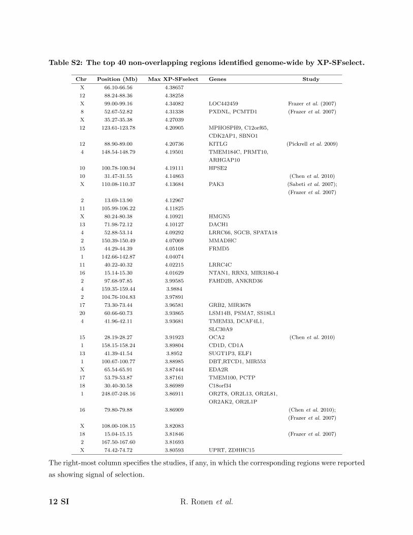
Table S2: The top 40 non-overlapping regions identified genome-wide by XP-SFselect.

Chr Position (Mb) Max XP-SFselect Genes Study

X 66.10-66.56 4.38657

12 88.24-88.36 4.38258

X 99.00-99.16 4.34082 LOC442459 Frazer et al. (2007)

8 52.67-52.82 4.31338 PXDNL, PCMTD1 (Frazer et al. 2007)

X 35.27-35.38 4.27039

12 123.61-123.78 4.20905 MPHOSPH9, C12orf65,

CDK2AP1, SBNO1

12 88.90-89.00 4.20736 KITLG (Pickrell et al. 2009)

4 148.54-148.79 4.19501 TMEM184C, PRMT10,

ARHGAP10

10 100.78-100.94 4.19111 HPSE2

10 31.47-31.55 4.14863 (Chen et al. 2010)

X 110.08-110.37 4.13684 PAK3 (Sabeti et al. 2007);

(Frazer et al. 2007)

2 13.69-13.90 4.12967

11 105.99-106.22 4.11825

X 80.24-80.38 4.10921 HMGN5

13 71.98-72.12 4.10127 DACH1

4 52.88-53.14 4.09292 LRRC66, SGCB, SPATA18

2 150.39-150.49 4.07069 MMADHC

15 44.29-44.39 4.05108 FRMD5

1 142.66-142.87 4.04074

11 40.22-40.32 4.02215 LRRC4C

16 15.14-15.30 4.01629 NTAN1, RRN3, MIR3180-4

2 97.68-97.85 3.99585 FAHD2B, ANKRD36

4 159.35-159.44 3.9884

2 104.76-104.83 3.97891

17 73.30-73.44 3.96581 GRB2, MIR3678

20 60.66-60.73 3.93865 LSM14B, PSMA7, SS18L1

4 41.96-42.11 3.93681 TMEM33, DCAF4L1,

SLC30A9

15 28.19-28.27 3.91923 OCA2 (Chen et al. 2010)

1 158.15-158.24 3.89804 CD1D, CD1A

13 41.39-41.54 3.8952 SUGT1P3, ELF1

1 100.67-100.77 3.88985 DBT,RTCD1, MIR553

X 65.54-65.91 3.87444 EDA2R

17 53.79-53.87 3.87161 TMEM100, PCTP

18 30.40-30.58 3.86989 C18orf34

1 248.07-248.16 3.86911 OR2T8, OR2L13, OR2L81,

OR2AK2, OR2L1P

16 79.80-79.88 3.86909 (Chen et al. 2010);

(Frazer et al. 2007)

X 108.00-108.15 3.82083

18 15.04-15.15 3.81846 (Frazer et al. 2007)

2 167.50-167.60 3.81693

X 74.42-74.72 3.80593 UPRT, ZDHHC15

The right-most column specifies the studies, if any, in which the corresponding regions were reported

as showing signal of selection.

12 SI R. Ronen et al.

Table S3: Potentially damaging SNPs found in regions with strong evidence of non-

neutral evolution.

Chr Position rsID AA SIFT Gene ENSEMBL CEU YRI

1 11090916 rs12711521 D371Y p = 0.04 MASP2 ENST00000400897 0.86 0.1

1 248084909 rs34508376 M197R p=0.01 OR2T8 ENST00000319968 0.64 0.05

1 248113026 rs10888281 Y289* — OR2L8 ENST00000357191 0.94 0.25

1 248129240 rs4478844 V203M p=0.00 OR2AK2 ENST00000366480 0.67 0.05

2 27424636 rs1395 S481F p=0.05 SLC5A6 ENST00000310574 0.74 0.16

5 138720108 rs11242462 W45* — SLC23A1 ENST00000508270 0.29 0.80

5 177378959 rs7720935 splice — RP11-423H2.3.1 ENST00000507072 0.94 0.40

8 16043667 rs435815 splice — MSR1 ENST00000445506 0.11 0.54

19 44932972 rs1434579 G662R p=0.04 ZNF229 ENST00000291187 0.40 0.04

20 2291722 rs6048066 I163L p=0.01 TGM3 ENST00000420960 0.006 0.49

SNPs found in the top 0.2% of XP-SFselect regions, deemed damaging by SIFT (nonsynonymous,

with p-value ≤ 0.05) or SnpEff (nonsense or splice-site variant). Frequencies in CEU and YRI

populations also shown. Splice site donor mutations are indicated by splice in the AA column.

R. Ronen et al. 13 SI