Learning Module 8 Shape · PDF file1 Learning Module 8 Shape Optimization Title Page Guide...
66
1 Learning Module 8 Shape Optimization Title Page Guide What is a Learning Module? A Learning Module (LM) is a structured, concise, and self-sufficient learning resource. An LM provides the learner with the required content in a precise and concise manner, enabling the learner to learn more efficiently and effectively. It has a number of characteristics that distinguish it from a traditional textbook or textbook chapter: An LM is learning objective driven, and its scope is clearly defined and bounded. The module is compact and precise in presentation, and its core material contains only contents essential for achieving the learning objectives. Since an LM is inherently concise, it can be learned relatively quickly and efficiently. An LM is independent and free-standing. Module-based learning is therefore non- sequential and flexible, and can be personalized with ease. Presenting the material in a contained and precise fashion will allow the user to learn effectively, reducing the time and effort spent and ultimately improving the learning experience. This is the first module on structural analysis and covers a static structural study in FEM. It goes through all of the steps necessary to successfully complete an analysis, including geometry creation, material selection, boundary condition specification, meshing, solution, and validation. These steps are first covered conceptually and then worked through directly as they are applied to an example problem. Estimated Learning Time for This Module Estimated learning time for this LM is equivalent to three 50-minute lectures, or one week of study time for a 3 credit hour course. How to Use This Module The learning module is organized in sections. Each section contains a short explanation and a link to where that section can be found. The explanation will give you an idea of what content is in each section. The link will allow you to complete the parts of the module you are interested in, while being able to skip any parts that you might already be familiar with. The modularity of the LM allows for an efficient use of your time.
-
Upload
truongdieu -
Category
Documents
-
view
231 -
download
1
Transcript of Learning Module 8 Shape · PDF file1 Learning Module 8 Shape Optimization Title Page Guide...

1
Learning Module 8
Shape Optimization
Title Page Guide
What is a Learning Module?
A Learning Module (LM) is a structured, concise, and self-sufficient learning
resource. An LM provides the learner with the required content in a precise and
concise manner, enabling the learner to learn more efficiently and effectively. It has a
number of characteristics that distinguish it from a traditional textbook or textbook
chapter:
An LM is learning objective driven, and its scope is clearly defined and bounded.
The module is compact and precise in presentation, and its core material contains
only contents essential for achieving the learning objectives. Since an LM is
inherently concise, it can be learned relatively quickly and efficiently.
An LM is independent and free-standing. Module-based learning is therefore non-
sequential and flexible, and can be personalized with ease.
Presenting the material in a contained and precise fashion will allow the user to learn
effectively, reducing the time and effort spent and ultimately improving the learning
experience. This is the first module on structural analysis and covers a static structural
study in FEM. It goes through all of the steps necessary to successfully complete an
analysis, including geometry creation, material selection, boundary condition
specification, meshing, solution, and validation. These steps are first covered
conceptually and then worked through directly as they are applied to an example
problem.
Estimated Learning Time for This Module
Estimated learning time for this LM is equivalent to three 50-minute lectures, or one
week of study time for a 3 credit hour course.
How to Use This Module
The learning module is organized in sections. Each section contains a short
explanation and a link to where that section can be found. The explanation will give
you an idea of what content is in each section. The link will allow you to complete the
parts of the module you are interested in, while being able to skip any parts that you
might already be familiar with. The modularity of the LM allows for an efficient use
of your time.
2
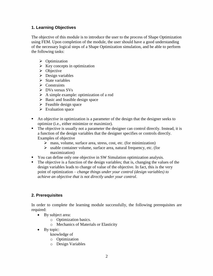
1. Learning Objectives
The objective of this module is to introduce the user to the process of Shape Optimization
using FEM. Upon completion of the module, the user should have a good understanding
of the necessary logical steps of a Shape Optimization simulation, and be able to perform
the following tasks:
Optimization
Key concepts in optimization
Objective
Design variables
State variables
Constraints
DVs versus SVs
A simple example: optimization of a rod
Basic and feasible design space
Feasible design space
Evaluation space
An objective in optimization is a parameter of the design that the designer seeks to
optimize (i.e., either minimize or maximize).
The objective is usually not a parameter the designer can control directly. Instead, it is
a function of the design variables that the designer specifies or controls directly.
Examples of objective
mass, volume, surface area, stress, cost, etc. (for minimization)
usable container volume, surface area, natural frequency, etc. (for
maximization)
You can define only one objective in SW Simulation optimization analysis.
The objective is a function of the design variables; that is, changing the values of the
design variables leads to change of value of the objective. In fact, this is the very
point of optimization – change things under your control (design variables) to
achieve an objective that is not directly under your control.
2. Prerequisites
In order to complete the learning module successfully, the following prerequisites are
required:
By subject area:
o Optimization basics.
o Mechanics of Materials or Elasticity
By topic:
knowledge of
o Optimization
o Design Variables
3
o State variables
o constraints
o feasible design
o displacement
o strain
o stress
o von Mises stress
o Saint Venant’s principle
o tension, bending, or torsion loading mode
4. Tutorial Problem Statements
A good tutorial problem should focus on the logical steps in FEM modeling and
demonstrate as many aspects of the FEM software as possible. It should also be simple in
mechanics with an analytical solution available for validation. Three tutorial problems are
covered in this learning module.
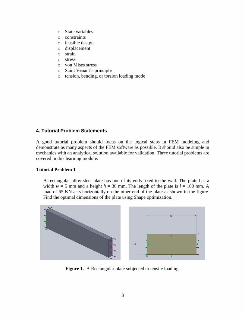
Tutorial Problem 1
A rectangular alloy steel plate has one of its ends fixed to the wall. The plate has a
width w = 5 mm and a height h = 30 mm. The length of the plate is l = 100 mm. A
load of 65 KN acts horizontally on the other end of the plate as shown in the figure.
Find the optimal dimensions of the plate using Shape optimization.
Figure 1. A Rectangular plate subjected to tensile loading.

4
Tutorial Problem 2
A rectangular alloy steel plate with a hole at its center has one of its ends fixed to the
wall. The plate has a width w = 5 mm and a height h = 50 mm. The hole dimensions
are shown in the below figure. The length of the plate is l = 100 mm. A tensile load of
46 KN magnitude acts horizontally on the other end of the plate. Find the optimal
dimensions of the plate using Shape optimization.
Figure 2. A rectangular plate with a hole at its center, rigidly fixed on one end and
loaded on the other end
5
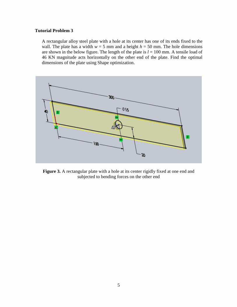
Tutorial Problem 3
A rectangular alloy steel plate with a hole at its center has one of its ends fixed to the
wall. The plate has a width w = 5 mm and a height h = 50 mm. The hole dimensions
are shown in the below figure. The length of the plate is l = 100 mm. A tensile load of
46 KN magnitude acts horizontally on the other end of the plate. Find the optimal
dimensions of the plate using Shape optimization.
Figure 3. A rectangular plate with a hole at its center rigidly fixed at one end and
subjected to bending forces on the other end
6
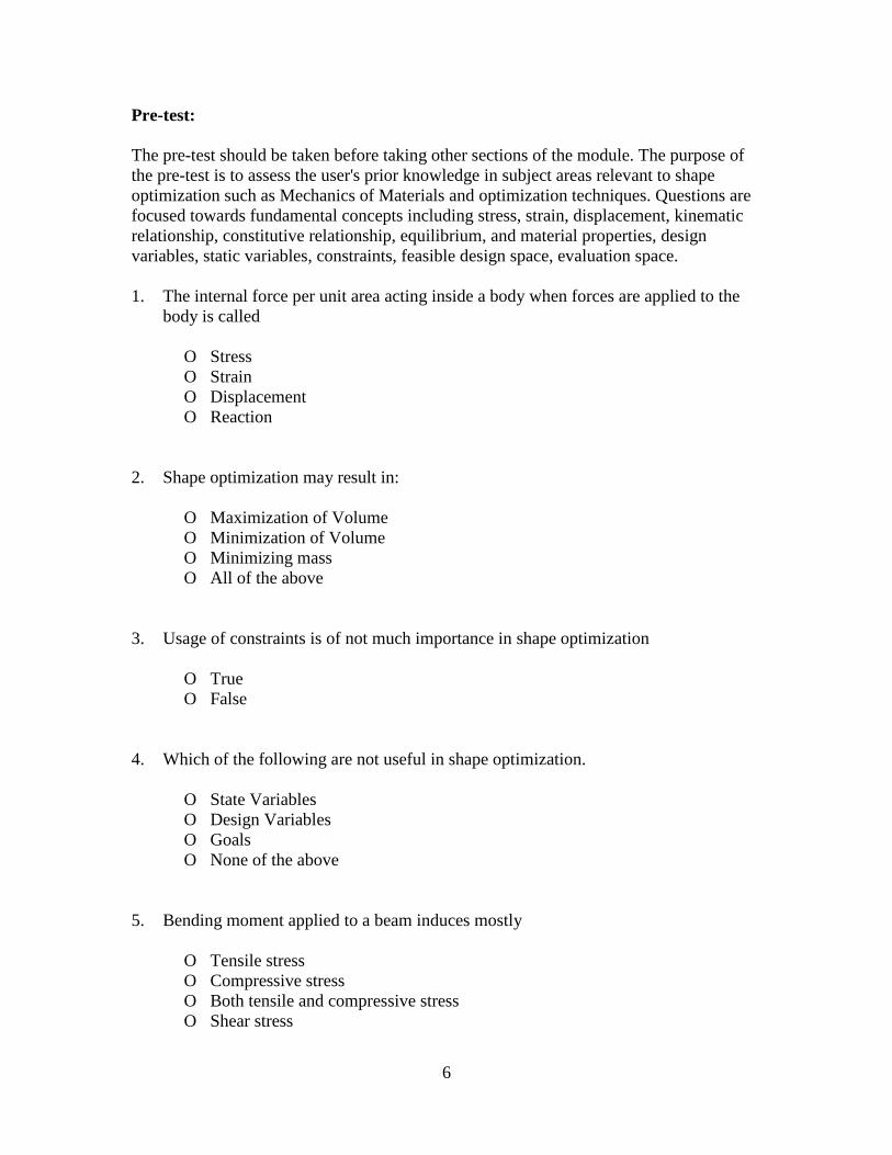
Pre-test:
The pre-test should be taken before taking other sections of the module. The purpose of
the pre-test is to assess the user's prior knowledge in subject areas relevant to shape
optimization such as Mechanics of Materials and optimization techniques. Questions are
focused towards fundamental concepts including stress, strain, displacement, kinematic
relationship, constitutive relationship, equilibrium, and material properties, design
variables, static variables, constraints, feasible design space, evaluation space.
1. The internal force per unit area acting inside a body when forces are applied to the
body is called
O Stress
O Strain
O Displacement
O Reaction
2. Shape optimization may result in:
O Maximization of Volume
O Minimization of Volume
O Minimizing mass
O All of the above
3. Usage of constraints is of not much importance in shape optimization
O True
O False
4. Which of the following are not useful in shape optimization.
O State Variables
O Design Variables
O Goals
O None of the above
5. Bending moment applied to a beam induces mostly
O Tensile stress
O Compressive stress
O Both tensile and compressive stress
O Shear stress
7
6. When the structure is made of same material, which of the following is true?
O Minimizing mass and maximizing volume is same.
O Minimizing mass and minimizing volume is same.
O Mass and Volume are not related
O None of the above.
7. For a bar of uniform cross-section under axial loading in x direction, the shape can
be optimized by considering the following constraints.
O Von-Mises stress, Displacement as variables & mass or volume as goal.
O Only volume or mass as goal.
O Only Von-Mises Stress, Displacement as variables.
O None of the above.
8. For a bar of uniform cross-section under axial loading in x direction, the Young’s
modulus is equal to
O The ratio of the axial displacement to the axial normal stress
O The ratio of the x-normal stress to the x-normal strain
O The ratio of the xy-shear stress to the x-normal stress
O The ratio of the xy-shear stress to the xy-shear strain
9. What is feasible design space?
10. Explain state variables, design variables and constraints
8
Conceptual Analysis of Shape Optimization:
Conceptual analysis for a Shape Optimization problem using finite element analysis
reveals that the following logical steps and sub-steps are needed:
Prerequisite (Associated) Study:
1. Preprocessing
Geometry creation
Material property assignment
Boundary conditions and loading
Mesh generation
2. Solution
3. Postprocessing
4. Validation
Optimization Study:
1. Preprocessing
Objective
Design variables
Constraints on state variables
2. Solution iterations
The above steps are explained in some detail as follows.
Prerequisite (Associated) Study:
1. Pre-processing
The pre-processing in FEM simulation is analogous to building the structure or making
the specimen in physical testing. Several sub-steps involved in pre-processing are
geometry creation, material property assignment, boundary condition specification, and
mesh generation.
The geometry of the structure to be analyzed is defined in the geometry creation step.
After the solid geometry is created, the material properties of the solid are specified in the
material property assignment step. The material required for the FEM analysis depends
on the type of analysis. For example, in the elastic deformation analysis of an isotropic
material under isothermal condition, only the modulus of elasticity and the Poisson’s
ratio are needed.
For most novice users of FEM, the boundary condition specification step is probably the
most challenging of all pre-processing steps. Two types of boundary conditions are
possible. The first is prescribed displacement boundary condition which is analogous to

9
holding or supporting the specimen in physical testing. The second is applied force
boundary condition which is analogous to loading the specimen. Several factors
contribute to the challenge of applying boundary conditions correctly:
1) Prescribed displacement boundary conditions expressed in terms such as
constuaboundary or const
x
u
bboundary
are mathematical simplifications, and
frequently only represent supports in real structures approximately. As a result,
choosing a good approximate mathematical representation can be a challenge.
2) How a boundary is restrained depends also on the element type. For example, for
the "clamped" or "built-in" support, a boundary should be restrained as having
zero nodal displacement if solid element is used, while for the same support, the
boundary should be restrained as having zero nodal displacement and zero nodal
rotation if shell element is used.
3) Frequently, the structure to be analyzed is not fully restrained from rigid body
motion in the original problem statement. In order to obtain an FEM solution,
auxiliary restraints become necessary. Over-restraining the model, however, leads
to spurious stress results. The challenge is then adding auxiliary restraints to
eliminate the possibility of rigid body motion without over-restraining the
structure.
Because of the above challenges, one learning module will be devoted to boundary
condition specification.
Mesh generation is the process of discretizing the body into finite elements and
assembling the discrete elements into an integral structure that approximates the original
body. Most FEM packages have their own default meshing parameters to mesh the model
and run the analysis while providing ways for the user to refine the mesh.
2. Solution
The solution is the process of solving the governing equations resulting from the
discretized FEM model. Although the mathematics for the solution process can be quite
involved, this step is transparent to the user and is usually as simple as clicking a solution
button or issuing the solution command.
3. Post-processing
The purpose of an FEM analysis is to obtain wanted results, and this is what the post-
processing step is for. Typically, various components or measures of stress, strain, and
displacement at any given location in the structure are available for putout. Additional
quantities for output may include factory of safety, energy norm error, contact pressure,
reaction force, strain energy density, etc. The way a quantity is outputted depends on the
FEM software.

10
Optimization Study:
1. Pre-processing
The objective of the optimization study is to get the optimized design for the given model
using the FEM package.
Select the desired optimization type (Minimize or Maximize), and the desired
objective from the dropdown menu (Mass, Volume, Frequency, Buckling)
In Response window, select the correct associated study
To define a Design Variable:
In the Design Variables column select Add parameter.
In the Lower Bound box, enter the smallest allowable dimension.
In the Upper Bound box, enter the largest allowable dimension.
Click OK.
To define Constraints on state variables:
Select the sensor type like simulation data, mass type and all.
Select the appropriate type of sensor.
Under Bounds, do the following:
Select the desired Units
In the Lower Bound box, enter the lowest allowable value for the SV.
In the Upper Bound box, enter the highest allowable value for the SV.
Click OK.
To define goals:
Sensor for goal is to be selected from the list of the sensors for mass or volume
which is to be maximized or minimized.
11
Overview: In this section, three tutorial problems will be solved using the commercial
FEM software SolidWorks. Although the underlying principles and logical steps of an
FEM simulation identified in the Conceptual Analysis section are independent of any
particular FEM software, the realization of conceptual analysis steps will be software
dependent. The SolidWorks-specific steps are described in this section.
This is a step-by-step tutorial. However, it is designed such that those who are familiar
with the details in a particular step can skip it and go directly into the next step.
Tutorial Problem 1. A rectangular beam subjected to tensile loading
0. Launching SolidWorks
SolidWorks Simulation is an integral part of the SolidWorks computer aided design
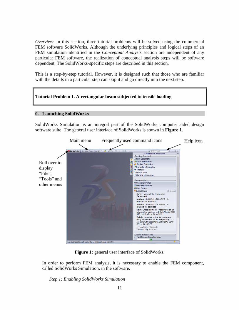
software suite. The general user interface of SolidWorks is shown in Figure 1.
Figure 1: general user interface of SolidWorks.
In order to perform FEM analysis, it is necessary to enable the FEM component,
called SolidWorks Simulation, in the software.
Step 1: Enabling SolidWorks Simulation
Main menu Frequently used command icons Help icon
Roll over to
display
“File”,
“Tools” and
other menus
12
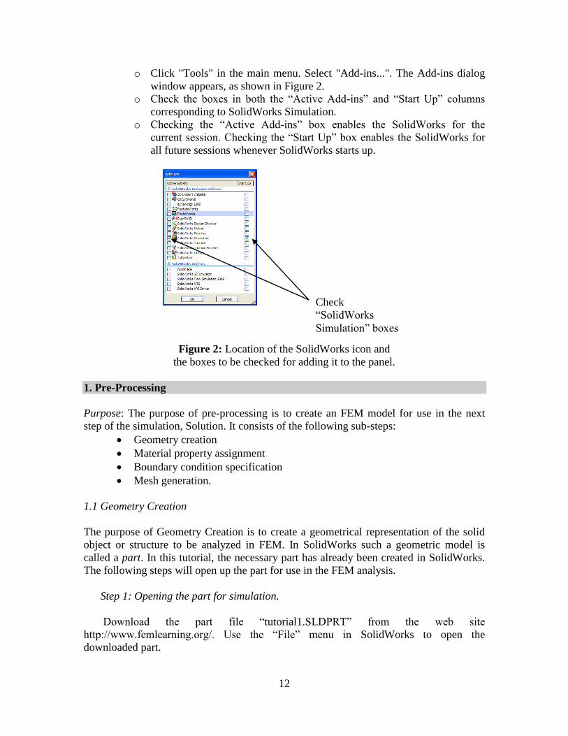
o Click "Tools" in the main menu. Select "Add-ins...". The Add-ins dialog
window appears, as shown in Figure 2.
o Check the boxes in both the “Active Add-ins” and “Start Up” columns
corresponding to SolidWorks Simulation.
o Checking the “Active Add-ins” box enables the SolidWorks for the
current session. Checking the “Start Up” box enables the SolidWorks for
all future sessions whenever SolidWorks starts up.
Figure 2: Location of the SolidWorks icon and
the boxes to be checked for adding it to the panel.
1. Pre-Processing
Purpose: The purpose of pre-processing is to create an FEM model for use in the next
step of the simulation, Solution. It consists of the following sub-steps:
Geometry creation
Material property assignment
Boundary condition specification
Mesh generation.
1.1 Geometry Creation
The purpose of Geometry Creation is to create a geometrical representation of the solid
object or structure to be analyzed in FEM. In SolidWorks such a geometric model is
called a part. In this tutorial, the necessary part has already been created in SolidWorks.
The following steps will open up the part for use in the FEM analysis.
Step 1: Opening the part for simulation.
Download the part file “tutorial1.SLDPRT” from the web site
http://www.femlearning.org/. Use the “File” menu in SolidWorks to open the
downloaded part.
Check
“SolidWorks
Simulation” boxes
13
The SolidWorks model tree will appear with the given part name at the top. Above the
model tree, there should be various tabs labeled “Features”, “Sketch”, etc. If the
“Simulation” tab is not visible, go back to steps 1 and 2 to enable the SolidWorks
Simulation package.
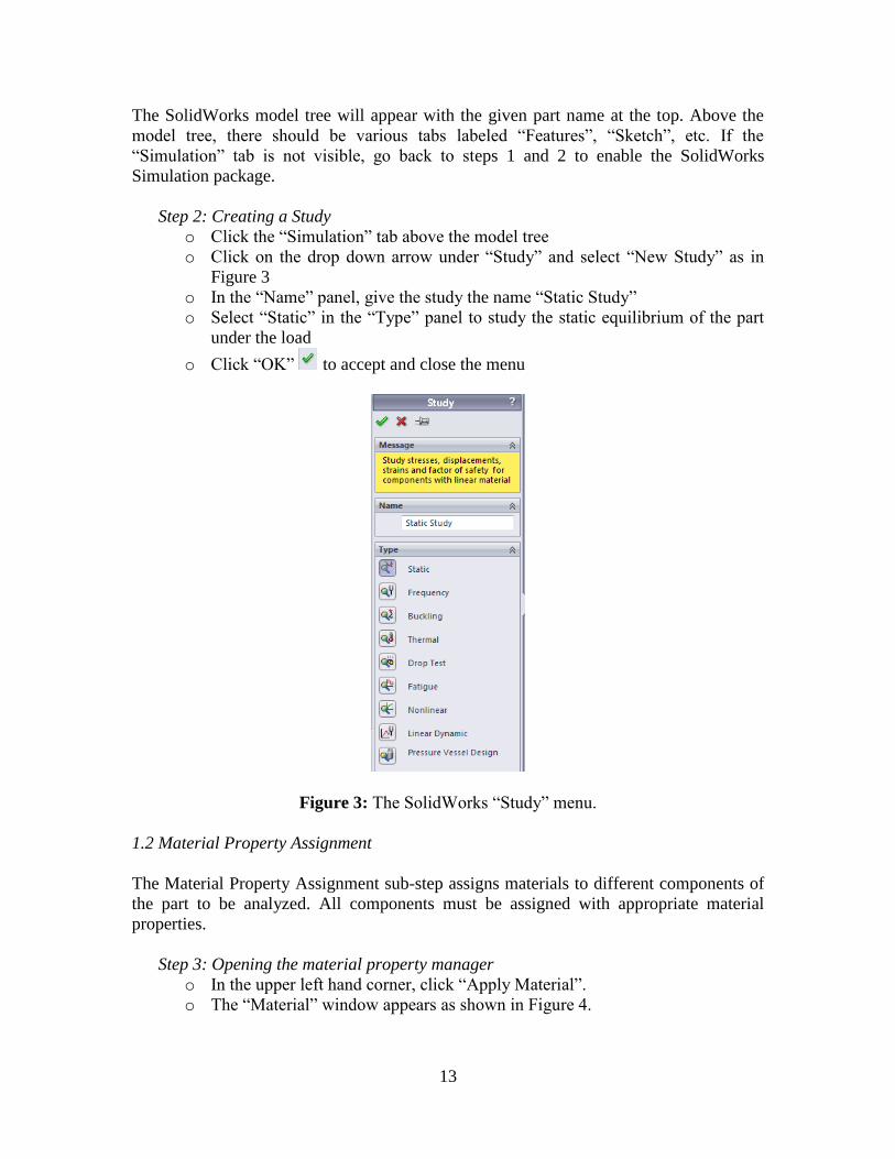
Step 2: Creating a Study
o Click the “Simulation” tab above the model tree
o Click on the drop down arrow under “Study” and select “New Study” as in
Figure 3
o In the “Name” panel, give the study the name “Static Study”
o Select “Static” in the “Type” panel to study the static equilibrium of the part
under the load
o Click “OK” to accept and close the menu
Figure 3: The SolidWorks “Study” menu.
1.2 Material Property Assignment
The Material Property Assignment sub-step assigns materials to different components of
the part to be analyzed. All components must be assigned with appropriate material
properties.
Step 3: Opening the material property manager
o In the upper left hand corner, click “Apply Material”.
o The “Material” window appears as shown in Figure 4.

14
Figure 4: The “Material” window.
This will apply one material to all components. If the part is made of several components
with different materials, open the model tree and apply this process to individual
components.
1.3 Boundary Condition Specification
In the Boundary Condition Specification sub-step, the restraints and loads on the part are
defined. Here, the face of the beam attached to the wall needs to be restrained, and the
force in the proper direction needs to be applied on the other end of the beam.
Step 5: Opening the fixtures property manager
o Right click on “Fixtures” in the model tree and select “Fixed Geometry”
o Move the cursor into the graphic window.
As the cursor traverses the image of the model, notice a small icon accompany the cursor,
and this icon change shapes when the cursor is at different locations. This indicates that
the SolidWorks is in graphical selection mode, and different shapes indicate different
identities would be selected: a square (icon) indicates the surface underneath the cursor
will be selected if the mouse is clicked, a line (icon) for an edge or a line, and a dot (icon)
for a point. In this tutorial problem, the entire end surface is restrained.

15
Figure 5: Applying an immovable restraint to the beam.
At the initial orientation, however, the end to be restrained is not visible, and could not be
selected. The model should be rotated to make the fixed end visible. To rotate the model
either hold down the scroll bar and rotate with the mouse or change the orientation by
clicking on the “View Orientation” icon in the top middle area of the workspace.
Once the desired face is visible, select the face on which to apply the restraint. Note that
in the display panel, within the second box in the “Type” panel, “Face<1>” appears,
indicating that one surface is being selected. Clicking on this face in the graphics panel
would deselect the face.
Step 6: Restraining the member
o Select the face as in Figure 5
o Once the face has been selected, click the green check mark to close the
“Fixture” menu
The next step is to load the beam with the applied force. The total force applied is 65000
N in the direction as shown in the figure 6.
16
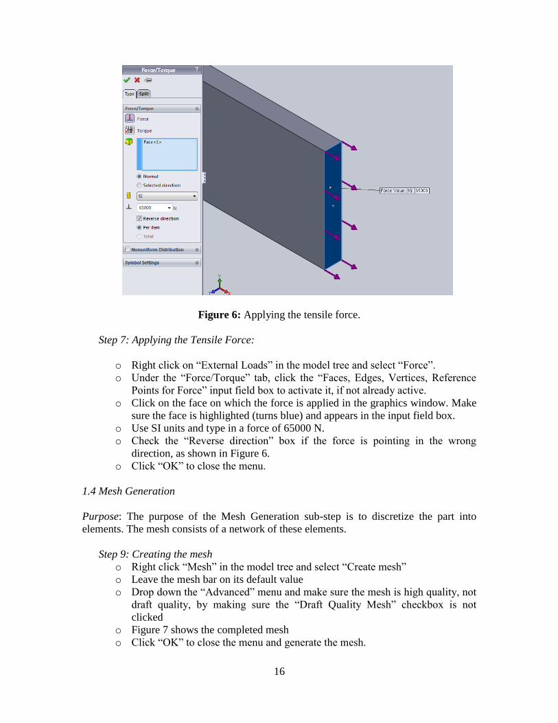
Figure 6: Applying the tensile force.
Step 7: Applying the Tensile Force:
o Right click on “External Loads” in the model tree and select “Force”.
o Under the “Force/Torque” tab, click the “Faces, Edges, Vertices, Reference
Points for Force” input field box to activate it, if not already active.
o Click on the face on which the force is applied in the graphics window. Make
sure the face is highlighted (turns blue) and appears in the input field box.
o Use SI units and type in a force of 65000 N.
o Check the “Reverse direction” box if the force is pointing in the wrong
direction, as shown in Figure 6.
o Click “OK” to close the menu.
1.4 Mesh Generation
Purpose: The purpose of the Mesh Generation sub-step is to discretize the part into
elements. The mesh consists of a network of these elements.
Step 9: Creating the mesh
o Right click “Mesh” in the model tree and select “Create mesh”
o Leave the mesh bar on its default value
o Drop down the “Advanced” menu and make sure the mesh is high quality, not
draft quality, by making sure the “Draft Quality Mesh” checkbox is not
clicked
o Figure 7 shows the completed mesh
o Click “OK” to close the menu and generate the mesh.

17
Figure 7: A completed mesh.
“Mesh Control” in SolidWorks may be used to refine the mesh locally. The guiding
principle is to refine mesh at locations of high stress gradient, such as regions around
stress concentrators and locations of geometric changes. For the current problem, local
mesh refinement is not pursued.
2. Solution
Purpose: The Solution is the step where the computer solves the simulation problem and
generates results for use in the Post-Processing step.
Step 1: Running the simulation
o At the top of the screen, click “Run”
o When the analysis is finished, the “Results” icon will appear on the model tree
3. Post-Processing
Purpose: The purpose of the Post-Processing step is to process the results of interest. For
this problem, the von Mises stress and the displacement is of interest.
Step 1: Creating a stress plot
o Right click “Results” on the model tree and select “Define Stress Plot”
o Select “von Mises” as the stress type and “Mpa” as the unit
o Unclick the “Deformed Shape” box and click “OK” to close the menu
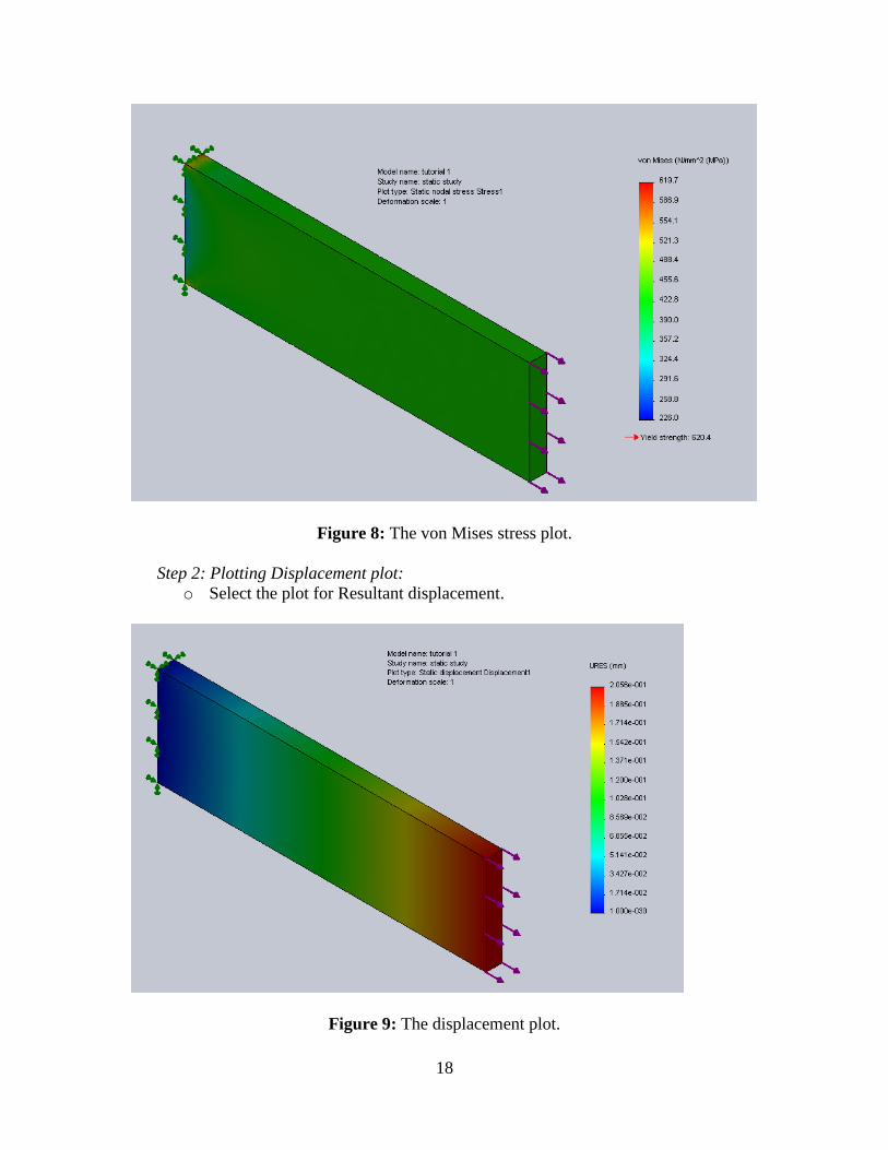
18
Figure 8: The von Mises stress plot.
Step 2: Plotting Displacement plot:
o Select the plot for Resultant displacement.
Figure 9: The displacement plot.
19
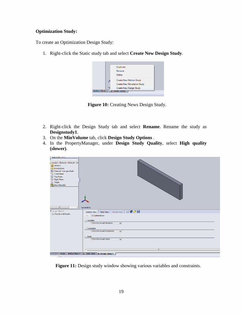
Optimization Study:
To create an Optimization Design Study:
1. Right-click the Static study tab and select Create New Design Study.
Figure 10: Creating News Design Study.
2. Right-click the Design Study tab and select Rename. Rename the study as
Designstudy1.
3. On the MinVolume tab, click Design Study Options .
4. In the PropertyManager, under Design Study Quality, select High quality
(slower).
Figure 11: Design study window showing various variables and constraints.
20
The program finds the optimal solution using many iterations with a Box-
Behnken design and displays the initial scenario, optimal scenario, and all
iterations. For more information about the quality of the study, see SolidWorks
Simulation Help: Properties for the Optimization Design Study.
5. Click Ok.
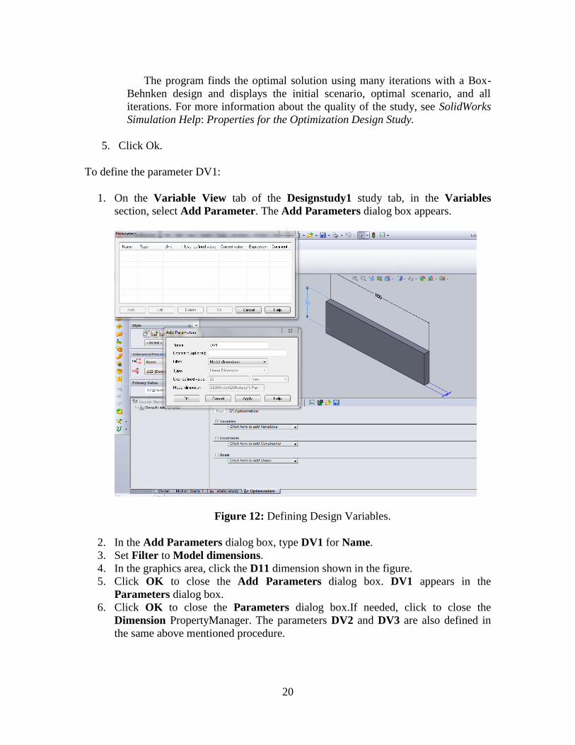
To define the parameter DV1:
1. On the Variable View tab of the Designstudy1 study tab, in the Variables
section, select Add Parameter. The Add Parameters dialog box appears.
Figure 12: Defining Design Variables.
2. In the Add Parameters dialog box, type DV1 for Name.
3. Set Filter to Model dimensions.
4. In the graphics area, click the D11 dimension shown in the figure.
5. Click OK to close the Add Parameters dialog box. DV1 appears in the
Parameters dialog box.
6. Click OK to close the Parameters dialog box.If needed, click to close the
Dimension PropertyManager. The parameters DV2 and DV3 are also defined in
the same above mentioned procedure.

21
To define the variables:
We define the three parameters named DV1, DV2, and DV3 as the variables.
1. On the Variable View tab of the Designstudy1 study tab, under Variables, select
DV1 (D11@Sketch1 in the sketch) from the list.
The selected variable appears in the Variables section.
32
Figure 13: Defining all Design Variables.
2. For the DV1 variable, select Range.
Figure 14: Defining type of
variable.
The program defines the
parameter as a continuous
variable for optimization. A
continuous variable is one
which can take any value
between the limits. For
example, 14.1567mm is a valid
value between a
minimum value of 25mm and a
maximum value of 35mm.
22
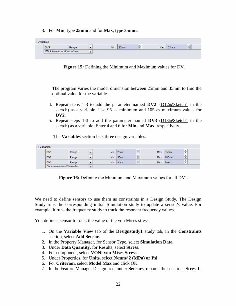
3. For Min, type 25mm and for Max, type 35mm.
Figure 15: Defining the Minimum and Maximum values for DV.
The program varies the model dimension between 25mm and 35mm to find the
optimal value for the variable.
4. Repeat steps 1-3 to add the parameter named DV2 (D12@Sketch1 in the
sketch) as a variable. Use 95 as minimum and 105 as maximum values for
DV2.
5. Repeat steps 1-3 to add the parameter named DV3 (D13@Sketch1 in the
sketch) as a variable. Enter 4 and 6 for Min and Max, respectively.
The Variables section lists three design variables.
Figure 16: Defining the Minimum and Maximum values for all DV’s.
We need to define sensors to use them as constraints in a Design Study. The Design
Study runs the corresponding initial Simulation study to update a sensor's value. For
example, it runs the frequency study to track the resonant frequency values.
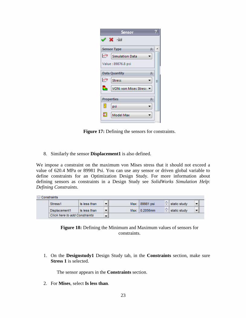
You define a sensor to track the value of the von Mises stress.
1. On the Variable View tab of the Designstudy1 study tab, in the Constraints
section, select Add Sensor.
2. In the Property Manager, for Sensor Type, select Simulation Data.
3. Under Data Quantity, for Results, select Stress.
4. For component, select VON: von Mises Stress.
5. Under Properties, for Units, select N/mm^2 (MPa) or Psi.
6. For Criterion, select Model Max and click OK.
7. In the Feature Manager Design tree, under Sensors, rename the sensor as Stress1.
23
Figure 17: Defining the sensors for constraints.
8. Similarly the sensor Displacement1 is also defined.
We impose a constraint on the maximum von Mises stress that it should not exceed a
value of 620.4 MPa or 89981 Psi. You can use any sensor or driven global variable to
define constraints for an Optimization Design Study. For more information about
defining sensors as constraints in a Design Study see SolidWorks Simulation Help:
Defining Constraints.
Figure 18: Defining the Minimum and Maximum values of sensors for
constraints.
1. On the Designstudy1 Design Study tab, in the Constraints section, make sure
Stress 1 is selected.
The sensor appears in the Constraints section.
2. For Mises, select Is less than.

24
3. For Max, type 620.4 N/mm^2.
The program automatically selects the Staticstudy study to run and track the
sensor's value since only one static study is defined.
Defining the Displacement constraint:
The maximum resultant displacement should not exceed 0.2056 mm.
1. On the Designstudy1 Design Study tab, in the Constraints section, from the list,
select URES.
The sensor appears in the Constraints section. This pre-defined sensor tracks
the value of resultant displacement.
2. For URES, select Is less than.
3. For Max, type 0.2056 mm.
The program automatically selects the Staticstudy study to run and track the
sensor's value.
Defining a goal:
The objective of this Optimization Design Study is to minimize the volume of the part.
Figure 19: Defining the Goal.
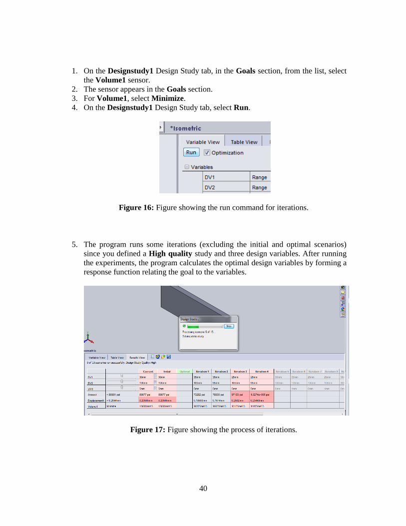
1. On the Designstudy1 Design Study tab, in the Goals section, from the list, select
the Volume1 sensor.
2. The sensor appears in the Goals section.
3. For Volume1, select Minimize.
4. On the Designstudy1 Design Study tab, select Run.
25
Figure 20: Figure showing the run command for iterations.
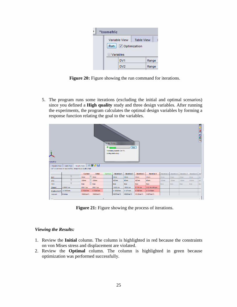
5. The program runs some iterations (excluding the initial and optimal scenarios)
since you defined a High quality study and three design variables. After running
the experiments, the program calculates the optimal design variables by forming a
response function relating the goal to the variables.
Figure 21: Figure showing the process of iterations.
Viewing the Results:
1. Review the Initial column. The column is highlighted in red because the constraints
on von Mises stress and displacement are violated.
2. Review the Optimal column. The column is highlighted in green because
optimization was performed successfully.

26
Figure 22: Figure showing the iterations.
The program updates the model with the optimal dimensions in the graphics window.
Figure 23: Figure showing the updated models with optimal values.
Study Results
15 of 15 iterations ran successfully.
Component
name
Units Current Initial Optimal Iteration1 Iteration2
DV1 mm 30.21393 30 30.21393 35 35
DV2 mm 95.06622 100 95.06622 105 95
DV3 mm 4.9267 5 4.9267 5 5
Stress1 psi 81015 89877 81015 73282 78930

27
Displacement1 mm 0.19697 0.20565 0.19697 0.18508 0.1674
Volume1 mm^3 14151.0696 15000 14151.0696 18375 16625
Component
name
Units Iteration3 Iteration4 Iteration5 Iteration6 Iteration7
DV1 mm 25 25 35 35 25
DV2 mm 105 95 100 100 100
DV3 mm 5 5 6 4 6
Stress1 psi 97103 1.0274e+005 68618 96292 89803
Displacement1 mm 0.2592 0.23449 0.14682 0.2203 0.20566
Volume1 mm^3 13125 11875 21000 14000 15000
Component
name
Units Iteration8 Iteration9 Iteration10 Iteration11 Iteration12
DV1 mm 25 30 30 30 30
DV2 mm 100 105 105 95 95
DV3 mm 4 6 4 6 4
Stress1 psi 1.2623e+005 69844 1.0965e+005 77742 1.0874e+005
Displacement1 mm 0.30858 0.17993 0.26998 0.16274 0.24417
Volume1 mm^3 10000 18900 12600 17100 11400
Component name Units Iteration13
DV1 mm 30
DV2 mm 100
DV3 mm 5
Stress1 psi 89877
Displacement1 mm 0.20565
Volume1 mm^3 15000
28
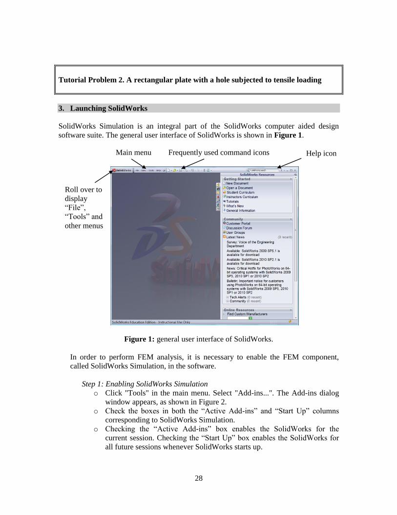
Tutorial Problem 2. A rectangular plate with a hole subjected to tensile loading
3. Launching SolidWorks
SolidWorks Simulation is an integral part of the SolidWorks computer aided design
software suite. The general user interface of SolidWorks is shown in Figure 1.
Figure 1: general user interface of SolidWorks.
In order to perform FEM analysis, it is necessary to enable the FEM component,
called SolidWorks Simulation, in the software.
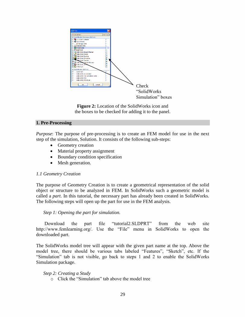
Step 1: Enabling SolidWorks Simulation
o Click "Tools" in the main menu. Select "Add-ins...". The Add-ins dialog
window appears, as shown in Figure 2.
o Check the boxes in both the “Active Add-ins” and “Start Up” columns
corresponding to SolidWorks Simulation.
o Checking the “Active Add-ins” box enables the SolidWorks for the
current session. Checking the “Start Up” box enables the SolidWorks for
all future sessions whenever SolidWorks starts up.
Main menu Frequently used command icons Help icon
Roll over to
display
“File”,
“Tools” and
other menus
29
Figure 2: Location of the SolidWorks icon and
the boxes to be checked for adding it to the panel.
1. Pre-Processing
Purpose: The purpose of pre-processing is to create an FEM model for use in the next
step of the simulation, Solution. It consists of the following sub-steps:
Geometry creation
Material property assignment
Boundary condition specification
Mesh generation.
1.1 Geometry Creation
The purpose of Geometry Creation is to create a geometrical representation of the solid
object or structure to be analyzed in FEM. In SolidWorks such a geometric model is
called a part. In this tutorial, the necessary part has already been created in SolidWorks.
The following steps will open up the part for use in the FEM analysis.
Step 1: Opening the part for simulation.
Download the part file “tutorial2.SLDPRT” from the web site
http://www.femlearning.org/. Use the “File” menu in SolidWorks to open the
downloaded part.
The SolidWorks model tree will appear with the given part name at the top. Above the
model tree, there should be various tabs labeled “Features”, “Sketch”, etc. If the
“Simulation” tab is not visible, go back to steps 1 and 2 to enable the SolidWorks
Simulation package.
Step 2: Creating a Study
o Click the “Simulation” tab above the model tree
Check
“SolidWorks
Simulation” boxes

30
o Click on the drop down arrow under “Study” and select “New Study” as in
Figure 3
o In the “Name” panel, give the study the name “Static Study”
o Select “Static” in the “Type” panel to study the static equilibrium of the part
under the load
o Click “OK” to accept and close the menu
Figure 3: The SolidWorks “Study” menu.
1.2 Material Property Assignment
The Material Property Assignment sub-step assigns materials to different components of
the part to be analyzed. All components must be assigned with appropriate material
properties.
Step 3: Opening the material property manager
o In the upper left hand corner, click “Apply Material”.
o The “Material” window appears as shown in Figure 4.
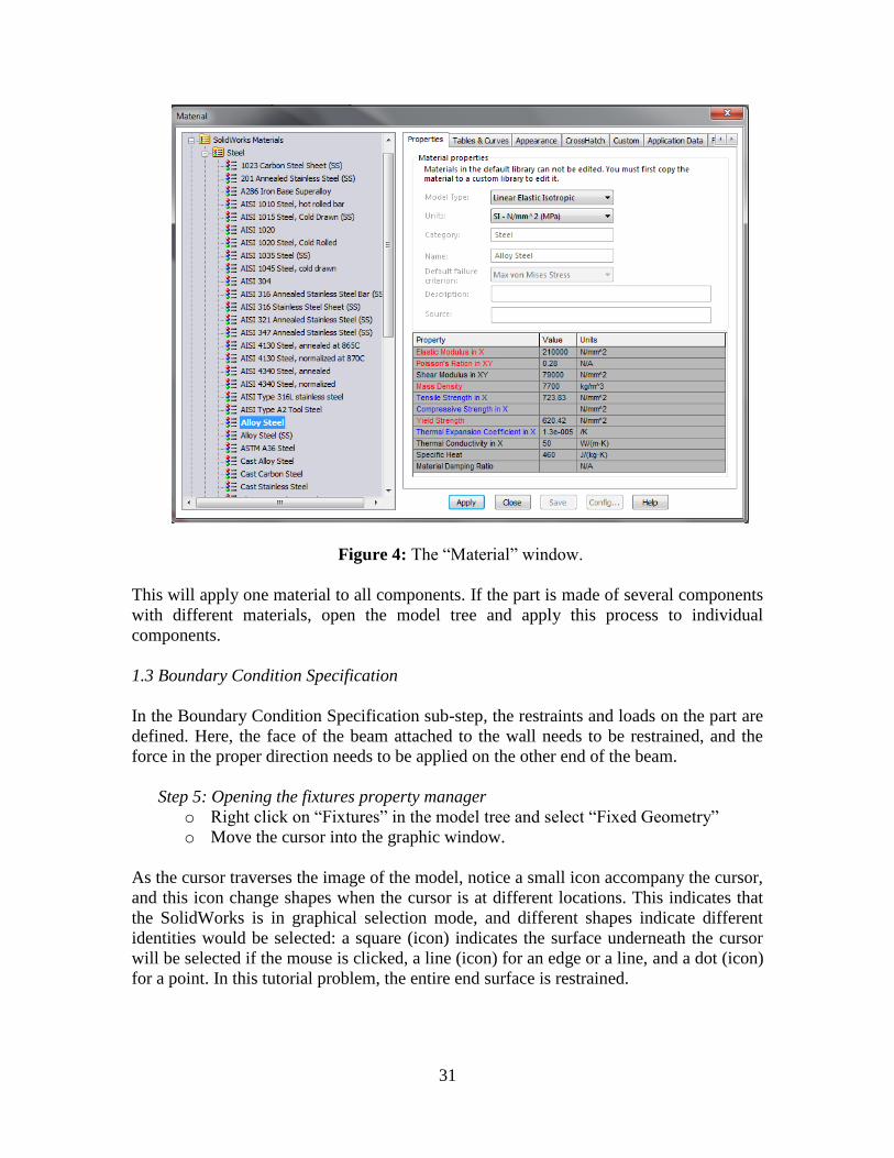
31
Figure 4: The “Material” window.
This will apply one material to all components. If the part is made of several components
with different materials, open the model tree and apply this process to individual
components.
1.3 Boundary Condition Specification
In the Boundary Condition Specification sub-step, the restraints and loads on the part are
defined. Here, the face of the beam attached to the wall needs to be restrained, and the
force in the proper direction needs to be applied on the other end of the beam.
Step 5: Opening the fixtures property manager
o Right click on “Fixtures” in the model tree and select “Fixed Geometry”
o Move the cursor into the graphic window.
As the cursor traverses the image of the model, notice a small icon accompany the cursor,
and this icon change shapes when the cursor is at different locations. This indicates that
the SolidWorks is in graphical selection mode, and different shapes indicate different
identities would be selected: a square (icon) indicates the surface underneath the cursor
will be selected if the mouse is clicked, a line (icon) for an edge or a line, and a dot (icon)
for a point. In this tutorial problem, the entire end surface is restrained.
32
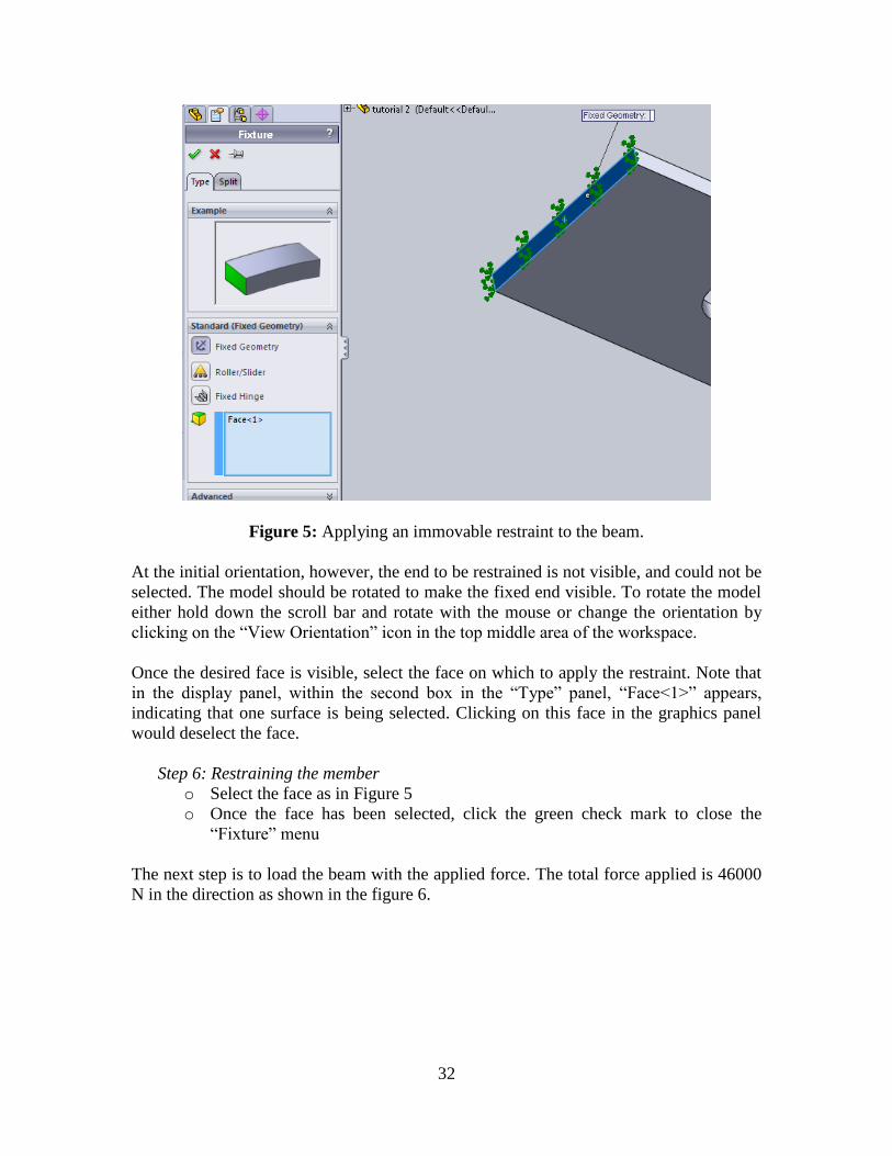
Figure 5: Applying an immovable restraint to the beam.
At the initial orientation, however, the end to be restrained is not visible, and could not be
selected. The model should be rotated to make the fixed end visible. To rotate the model
either hold down the scroll bar and rotate with the mouse or change the orientation by
clicking on the “View Orientation” icon in the top middle area of the workspace.
Once the desired face is visible, select the face on which to apply the restraint. Note that
in the display panel, within the second box in the “Type” panel, “Face<1>” appears,
indicating that one surface is being selected. Clicking on this face in the graphics panel
would deselect the face.
Step 6: Restraining the member
o Select the face as in Figure 5
o Once the face has been selected, click the green check mark to close the
“Fixture” menu
The next step is to load the beam with the applied force. The total force applied is 46000
N in the direction as shown in the figure 6.
33
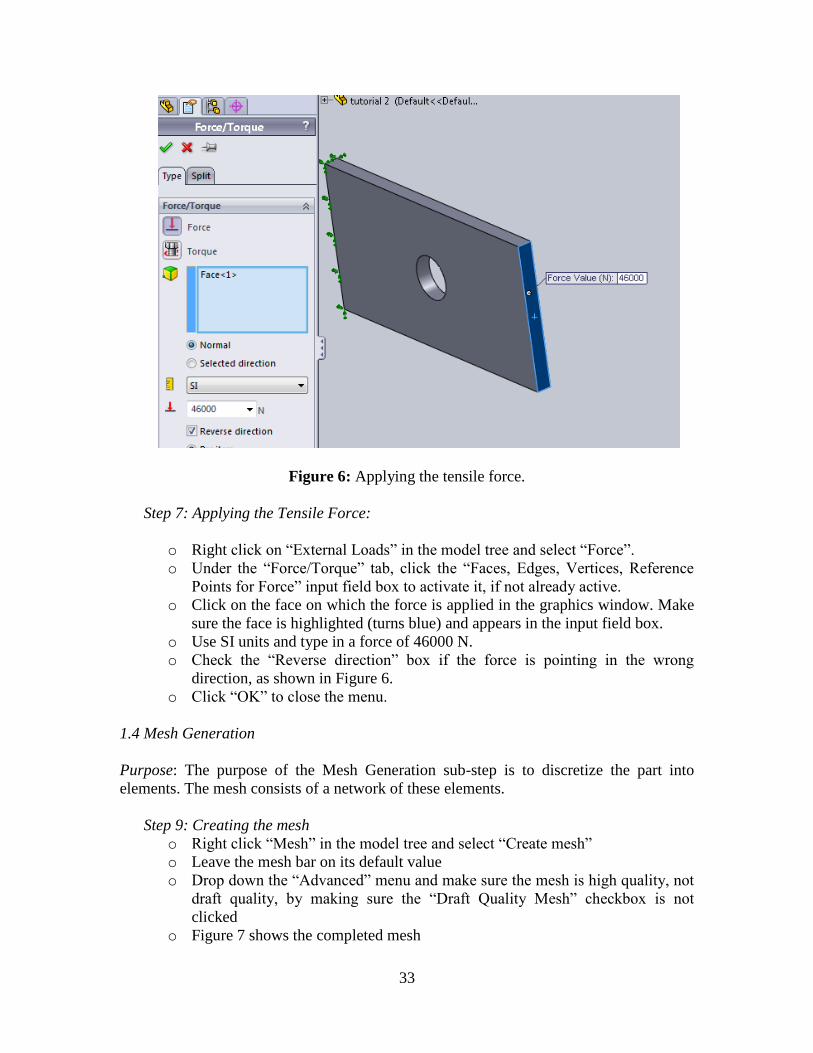
Figure 6: Applying the tensile force.
Step 7: Applying the Tensile Force:
o Right click on “External Loads” in the model tree and select “Force”.
o Under the “Force/Torque” tab, click the “Faces, Edges, Vertices, Reference
Points for Force” input field box to activate it, if not already active.
o Click on the face on which the force is applied in the graphics window. Make
sure the face is highlighted (turns blue) and appears in the input field box.
o Use SI units and type in a force of 46000 N.
o Check the “Reverse direction” box if the force is pointing in the wrong
direction, as shown in Figure 6.
o Click “OK” to close the menu.
1.4 Mesh Generation
Purpose: The purpose of the Mesh Generation sub-step is to discretize the part into
elements. The mesh consists of a network of these elements.
Step 9: Creating the mesh
o Right click “Mesh” in the model tree and select “Create mesh”
o Leave the mesh bar on its default value
o Drop down the “Advanced” menu and make sure the mesh is high quality, not
draft quality, by making sure the “Draft Quality Mesh” checkbox is not
clicked
o Figure 7 shows the completed mesh

34
o Click “OK” to close the menu and generate the mesh.
Figure 7: A completed mesh.
“Mesh Control” in SolidWorks may be used to refine the mesh locally. The guiding
principle is to refine mesh at locations of high stress gradient, such as regions around
stress concentrators and locations of geometric changes. For the current problem, local
mesh refinement is not pursued.
2. Solution
Purpose: The Solution is the step where the computer solves the simulation problem and
generates results for use in the Post-Processing step.
Step 1: Running the simulation
o At the top of the screen, click “Run”
o When the analysis is finished, the “Results” icon will appear on the model tree
3. Post-Processing
Purpose: The purpose of the Post-Processing step is to process the results of interest. For
this problem, the von Mises stress and the displacement is of interest.
Step 1: Creating a stress plot

35
o Right click “Results” on the model tree and select “Define Stress Plot”
o Select “von Mises” as the stress type and “Mpa” as the unit
o Unclick the “Deformed Shape” box and click “OK” to close the menu
Figure 8: The von Mises stress plot.
Step 2: Plotting Displacement plot:
o Select the plot for Resultant displacement.
Figure 9: The displacement plot.
36
Optimization Study:
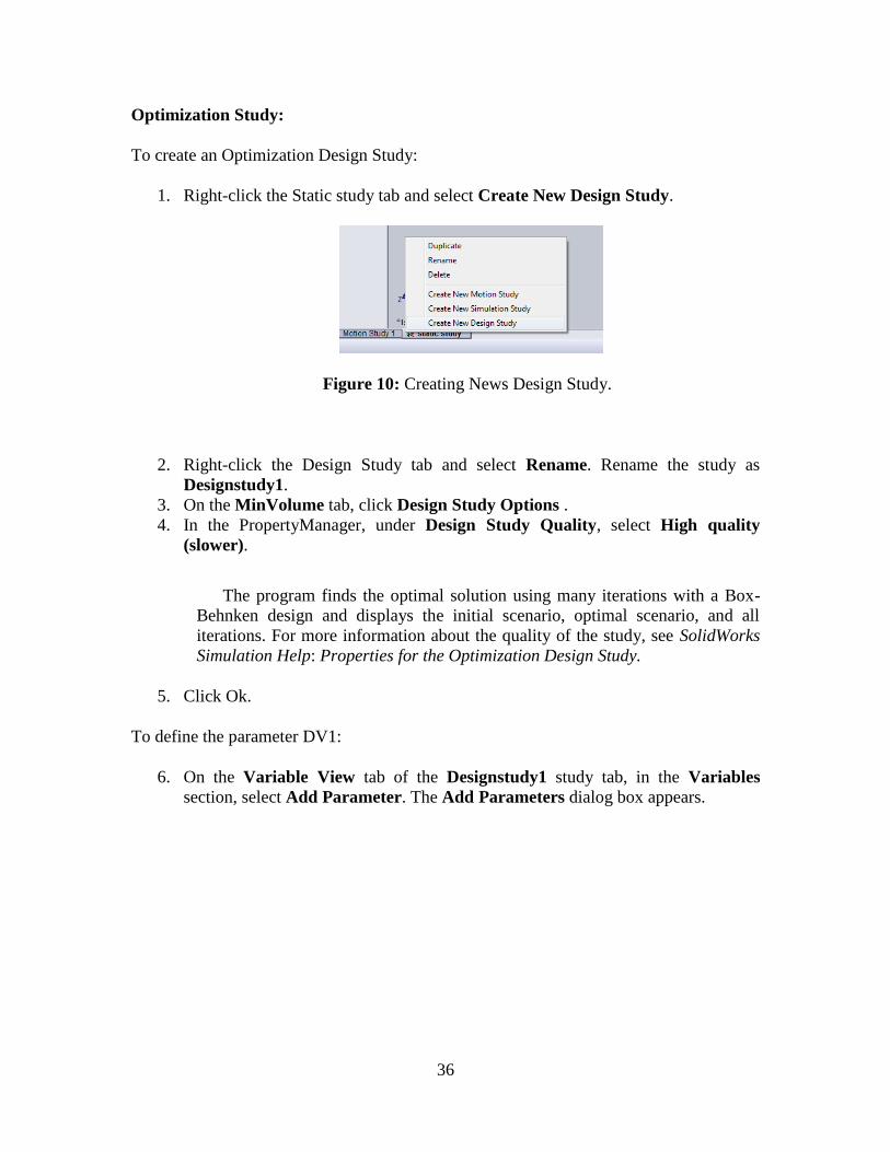
To create an Optimization Design Study:
1. Right-click the Static study tab and select Create New Design Study.
Figure 10: Creating News Design Study.
2. Right-click the Design Study tab and select Rename. Rename the study as
Designstudy1.
3. On the MinVolume tab, click Design Study Options .
4. In the PropertyManager, under Design Study Quality, select High quality
(slower).
The program finds the optimal solution using many iterations with a Box-
Behnken design and displays the initial scenario, optimal scenario, and all
iterations. For more information about the quality of the study, see SolidWorks
Simulation Help: Properties for the Optimization Design Study.
5. Click Ok.
To define the parameter DV1:
6. On the Variable View tab of the Designstudy1 study tab, in the Variables
section, select Add Parameter. The Add Parameters dialog box appears.
37
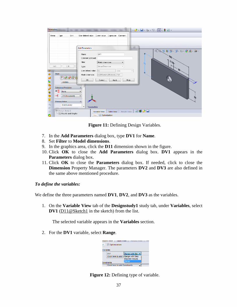
Figure 11: Defining Design Variables.
7. In the Add Parameters dialog box, type DV1 for Name.
8. Set Filter to Model dimensions.
9. In the graphics area, click the D11 dimension shown in the figure.
10. Click OK to close the Add Parameters dialog box. DV1 appears in the
Parameters dialog box.
11. Click OK to close the Parameters dialog box. If needed, click to close the
Dimension Property Manager. The parameters DV2 and DV3 are also defined in
the same above mentioned procedure.
To define the variables:
We define the three parameters named DV1, DV2, and DV3 as the variables.
1. On the Variable View tab of the Designstudy1 study tab, under Variables, select
DV1 (D11@Sketch1 in the sketch) from the list.
The selected variable appears in the Variables section.
2. For the DV1 variable, select Range.
Figure 12: Defining type of variable.

38
3. The program defines the parameter as a continuous variable for optimization. A
continuous variable is one which can take any value between the limits. For
example, 14.1567mm is a valid value between a minimum value of 45mm and a
maximum value of 55mm.
4. The program varies the model dimension between 25mm and 35mm to find the
optimal value for the variable.
5. Repeat steps 1-3 to add the parameter named DV2 through DV6.
The Variables section lists three design variables.
Figure 13: Defining the Minimum and Maximum values for all DV’s.
We need to define sensors to use them as constraints in a Design Study. The Design
Study runs the corresponding initial Simulation study to update a sensor's value. For
example, it runs the frequency study to track the resonant frequency values.
We define a sensor to track the value of the von Mises stress.
1. On the Variable View tab of the Designstudy1 study tab, in the Constraints
section, select Add Sensor.
2. In the Property Manager, for Sensor Type, select Simulation Data.
3. Under Data Quantity, for Results, select Stress.
4. For component, select VON: von Mises Stress.
5. Under Properties, for Units, select N/mm^2 (MPa) or Psi.
6. For Criterion, select Model Max and click OK.
7. In the Feature Manager Design tree, under Sensors, rename the sensor as Stress1.
8. Similarly the sensor Displacement1 is also defined as like in the tutorial1.
We impose a constraint on the maximum von Mises stress that it should not exceed a
value of 620.4 MPa or 89981 Psi. You can use any sensor or driven global variable to
define constraints for an Optimization Design Study. For more information about
defining sensors as constraints in a Design Study see SolidWorks Simulation Help:
39
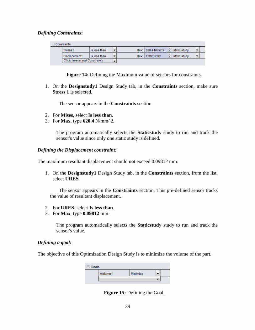
Defining Constraints:
Figure 14: Defining the Maximum value of sensors for constraints.
1. On the Designstudy1 Design Study tab, in the Constraints section, make sure
Stress 1 is selected.
The sensor appears in the Constraints section.
2. For Mises, select Is less than.
3. For Max, type 620.4 N/mm^2.
The program automatically selects the Staticstudy study to run and track the
sensor's value since only one static study is defined.
Defining the Displacement constraint:
The maximum resultant displacement should not exceed 0.09812 mm.
1. On the Designstudy1 Design Study tab, in the Constraints section, from the list,
select URES.
The sensor appears in the Constraints section. This pre-defined sensor tracks
the value of resultant displacement.
2. For URES, select Is less than.
3. For Max, type 0.09812 mm.
The program automatically selects the Staticstudy study to run and track the
sensor's value.
Defining a goal:
The objective of this Optimization Design Study is to minimize the volume of the part.
Figure 15: Defining the Goal.
40
1. On the Designstudy1 Design Study tab, in the Goals section, from the list, select
the Volume1 sensor.
2. The sensor appears in the Goals section.
3. For Volume1, select Minimize.
4. On the Designstudy1 Design Study tab, select Run.
Figure 16: Figure showing the run command for iterations.
5. The program runs some iterations (excluding the initial and optimal scenarios)
since you defined a High quality study and three design variables. After running
the experiments, the program calculates the optimal design variables by forming a
response function relating the goal to the variables.
Figure 17: Figure showing the process of iterations.

41
Viewing the Results:
1. Review the Initial column. The column is highlighted in red because the constraints
on von Mises stress and displacement are violated.
2. Review the Optimal column. The column is highlighted in green because
optimization was performed successfully.
Figure 18: Figure showing the iterations.
The program updates the model with the optimal dimensions in the graphics window.
Figure 19: Figure showing the updated models with optimal values.

42
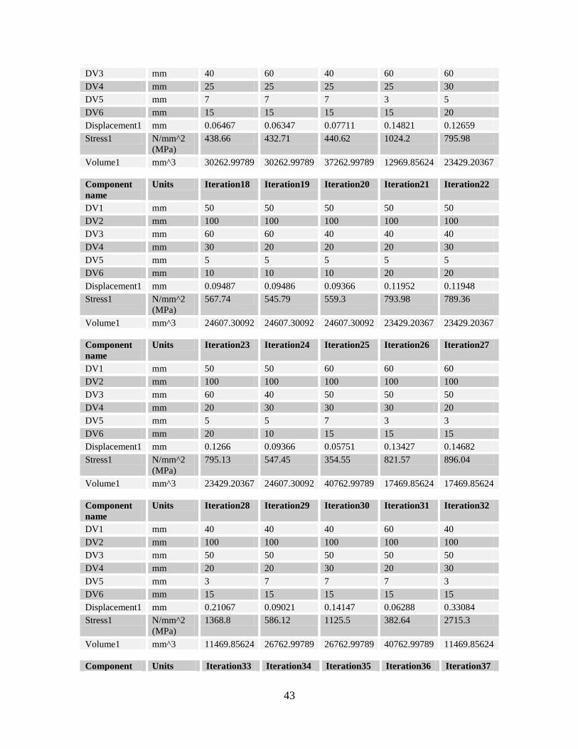
Study Results
51 of 51 iterations ran successfully.
Component
name
Units Current Initial Optimal Iteration1 Iteration2
DV1 mm 50 53.63739 50 60 60
DV2 mm 100 95.82489 100 110 110
DV3 mm 50 49.86481 50 50 50
DV4 mm 25 24.87213 25 30 20
DV5 mm 5 4.24872 5 5 5
DV6 mm 15 12.73483 15 15 15
Displacement1 mm 0.09812 0.10017 0.09812 0.08779 0.09517
Stress1 N/mm^2
(MPa)
619.37 641.2 619.37 486.52 542.83
Volume1 mm^3 24116.42707 21296.37871 24116.42707 32116.42707 32116.42707
Component
name
Units Iteration3 Iteration4 Iteration5 Iteration6 Iteration7
DV1 mm 60 40 40 40 60
DV2 mm 90 90 90 110 90
DV3 mm 50 50 50 50 50
DV4 mm 20 20 30 30 30
DV5 mm 5 5 5 5 5
DV6 mm 15 15 15 15 15
Displacement1 mm 0.081 0.11553 0.1889 0.20796 0.07325
Stress1 N/mm^2
(MPa)
530.73 832.33 1594.8 1571.1 497.45
Volume1 mm^3 26116.42707 17116.42707 17116.42707 21116.42707 26116.42707
Component
name
Units Iteration8 Iteration9 Iteration10 Iteration11 Iteration12
DV1 mm 40 50 50 50 50
DV2 mm 110 110 110 110 90
DV3 mm 50 60 60 40 40
DV4 mm 20 25 25 25 25
DV5 mm 5 7 3 3 3
DV6 mm 15 15 15 15 15
Displacement1 mm 0.13726 0.07599 0.17742 0.18 0.15098
Stress1 N/mm^2
(MPa)
817.05 437.4 1034.4 1026.6 1033.3
Volume1 mm^3 21116.42707 37262.99789 15969.85624 15969.85624 12969.85624
Component
name
Units Iteration13 Iteration14 Iteration15 Iteration16 Iteration17
DV1 mm 50 50 50 50 50
DV2 mm 90 90 110 90 100
43
DV3 mm 40 60 40 60 60
DV4 mm 25 25 25 25 30
DV5 mm 7 7 7 3 5
DV6 mm 15 15 15 15 20
Displacement1 mm 0.06467 0.06347 0.07711 0.14821 0.12659
Stress1 N/mm^2
(MPa)
438.66 432.71 440.62 1024.2 795.98
Volume1 mm^3 30262.99789 30262.99789 37262.99789 12969.85624 23429.20367
Component
name
Units Iteration18 Iteration19 Iteration20 Iteration21 Iteration22
DV1 mm 50 50 50 50 50
DV2 mm 100 100 100 100 100
DV3 mm 60 60 40 40 40
DV4 mm 30 20 20 20 30
DV5 mm 5 5 5 5 5
DV6 mm 10 10 10 20 20
Displacement1 mm 0.09487 0.09486 0.09366 0.11952 0.11948
Stress1 N/mm^2
(MPa)
567.74 545.79 559.3 793.98 789.36
Volume1 mm^3 24607.30092 24607.30092 24607.30092 23429.20367 23429.20367
Component
name
Units Iteration23 Iteration24 Iteration25 Iteration26 Iteration27
DV1 mm 50 50 60 60 60
DV2 mm 100 100 100 100 100
DV3 mm 60 40 50 50 50
DV4 mm 20 30 30 30 20
DV5 mm 5 5 7 3 3
DV6 mm 20 10 15 15 15
Displacement1 mm 0.1266 0.09366 0.05751 0.13427 0.14682
Stress1 N/mm^2
(MPa)
795.13 547.45 354.55 821.57 896.04
Volume1 mm^3 23429.20367 24607.30092 40762.99789 17469.85624 17469.85624
Component
name
Units Iteration28 Iteration29 Iteration30 Iteration31 Iteration32
DV1 mm 40 40 40 60 40
DV2 mm 100 100 100 100 100
DV3 mm 50 50 50 50 50
DV4 mm 20 20 30 20 30
DV5 mm 3 7 7 7 3
DV6 mm 15 15 15 15 15
Displacement1 mm 0.21067 0.09021 0.14147 0.06288 0.33084
Stress1 N/mm^2
(MPa)
1368.8 586.12 1125.5 382.64 2715.3
Volume1 mm^3 11469.85624 26762.99789 26762.99789 40762.99789 11469.85624
Component Units Iteration33 Iteration34 Iteration35 Iteration36 Iteration37

44
name
DV1 mm 50 50 50 50 50
DV2 mm 110 110 110 90 90
DV3 mm 50 50 50 50 50
DV4 mm 25 25 25 25 25
DV5 mm 7 7 3 3 3
DV6 mm 20 10 10 10 20
Displacement1 mm 0.08372 0.07168 0.16735 0.13827 0.16655
Stress1 N/mm^2
(MPa)
480.91 399.61 933.51 942.7 1159.1
Volume1 mm^3 36300.88514 37950.22129 16264.38055 13264.38055 12557.5222
Component
name
Units Iteration38 Iteration39 Iteration40 Iteration41 Iteration42
DV1 mm 50 50 50 60 60
DV2 mm 90 110 90 100 100
DV3 mm 50 50 50 60 60
DV4 mm 25 25 25 25 25
DV5 mm 7 3 7 5 5
DV6 mm 20 20 10 20 10
Displacement1 mm 0.07133 0.19545 0.05921 0.09392 0.07733
Stress1 N/mm^2
(MPa)
481.89 1157.8 403.68 573.52 448.27
Volume1 mm^3 29300.88514 15557.5222 30950.22129 28429.20367 29607.30092
Component
name
Units Iteration43 Iteration44 Iteration45 Iteration46 Iteration47
DV1 mm 60 40 40 40 60
DV2 mm 100 100 100 100 100
DV3 mm 40 40 40 60 40
DV4 mm 25 25 25 25 25
DV5 mm 5 5 5 5 5
DV6 mm 10 10 20 20 20
Displacement1 mm 0.07662 0.12207 0.19231 0.20968 0.09177
Stress1 N/mm^2
(MPa)
442.92 733.82 1353.1 1358.2 584.67
Volume1 mm^3 29607.30092 19607.30092 18429.20367 18429.20367 28429.20367
Component name Units Iteration48 Iteration49
DV1 mm 40 50
DV2 mm 100 100
DV3 mm 60 50
DV4 mm 25 25
DV5 mm 5 5
DV6 mm 10 15
Displacement1 mm 0.12346 0.09812
Stress1 N/mm^2 (MPa) 734.24 619.37
Volume1 mm^3 19607.30092 24116.42707

45
Tutorial Problem 3. A rectangular plate with a hole subjected to bending loading
Launching SolidWorks
SolidWorks Simulation is an integral part of the SolidWorks computer aided design
software suite. The general user interface of SolidWorks is shown in Figure 1.
Figure 1: general user interface of SolidWorks.
In order to perform FEM analysis, it is necessary to enable the FEM component,
called SolidWorks Simulation, in the software.
Step 1: Enabling SolidWorks Simulation
o Click "Tools" in the main menu. Select "Add-ins...". The Add-ins dialog
window appears, as shown in Figure 2.
o Check the boxes in both the “Active Add-ins” and “Start Up” columns
corresponding to SolidWorks Simulation.
o Checking the “Active Add-ins” box enables the SolidWorks for the
current session. Checking the “Start Up” box enables the SolidWorks for
all future sessions whenever SolidWorks starts up.
Main menu Frequently used command icons Help icon
Roll over to
display
“File”,
“Tools” and
other menus

46
Figure 2: Location of the SolidWorks icon and
the boxes to be checked for adding it to the panel.
1. Pre-Processing
Purpose: The purpose of pre-processing is to create an FEM model for use in the next
step of the simulation, Solution. It consists of the following sub-steps:
Geometry creation
Material property assignment
Boundary condition specification
Mesh generation.
1.1 Geometry Creation
The purpose of Geometry Creation is to create a geometrical representation of the solid
object or structure to be analyzed in FEM. In SolidWorks such a geometric model is
called a part. In this tutorial, the necessary part has already been created in SolidWorks.
The following steps will open up the part for use in the FEM analysis.
Step 1: Opening the part for simulation.
Download the part file “tutorial3.SLDPRT” from the web site
http://www.femlearning.org/. Use the “File” menu in SolidWorks to open the
downloaded part.
The SolidWorks model tree will appear with the given part name at the top. Above the
model tree, there should be various tabs labeled “Features”, “Sketch”, etc. If the
“Simulation” tab is not visible, go back to steps 1 and 2 to enable the SolidWorks
Simulation package.
Step 2: Creating a Study
o Click the “Simulation” tab above the model tree
Check
“SolidWorks
Simulation” boxes

47
o Click on the drop down arrow under “Study” and select “New Study” as in
Figure 3
o In the “Name” panel, give the study the name “Static Study”
o Select “Static” in the “Type” panel to study the static equilibrium of the part
under the load
o Click “OK” to accept and close the menu
Figure 3: The SolidWorks “Study” menu.
1.2 Material Property Assignment
The Material Property Assignment sub-step assigns materials to different components of
the part to be analyzed. All components must be assigned with appropriate material
properties.
Step 3: Opening the material property manager
o In the upper left hand corner, click “Apply Material”.
o The “Material” window appears as shown in Figure 4.

48
Figure 4: The “Material” window.
This will apply one material to all components. If the part is made of several components
with different materials, open the model tree and apply this process to individual
components.
1.3 Boundary Condition Specification
In the Boundary Condition Specification sub-step, the restraints and loads on the part are
defined. Here, the face of the beam attached to the wall needs to be restrained, and the
force in the proper direction needs to be applied on the other end of the beam.
Step 4: Opening the fixtures property manager
o Right click on “Fixtures” in the model tree and select “Fixed Geometry”
o Move the cursor into the graphic window.
As the cursor traverses the image of the model, notice a small icon accompany the cursor,
and this icon change shapes when the cursor is at different locations. This indicates that
the SolidWorks is in graphical selection mode, and different shapes indicate different
identities would be selected: a square (icon) indicates the surface underneath the cursor
will be selected if the mouse is clicked, a line (icon) for an edge or a line, and a dot (icon)
for a point. In this tutorial problem, the entire end surface is restrained.
49
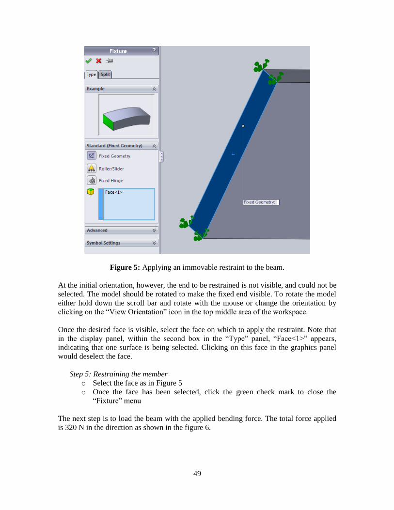
Figure 5: Applying an immovable restraint to the beam.
At the initial orientation, however, the end to be restrained is not visible, and could not be
selected. The model should be rotated to make the fixed end visible. To rotate the model
either hold down the scroll bar and rotate with the mouse or change the orientation by
clicking on the “View Orientation” icon in the top middle area of the workspace.
Once the desired face is visible, select the face on which to apply the restraint. Note that
in the display panel, within the second box in the “Type” panel, “Face<1>” appears,
indicating that one surface is being selected. Clicking on this face in the graphics panel
would deselect the face.
Step 5: Restraining the member
o Select the face as in Figure 5
o Once the face has been selected, click the green check mark to close the
“Fixture” menu
The next step is to load the beam with the applied bending force. The total force applied
is 320 N in the direction as shown in the figure 6.
50
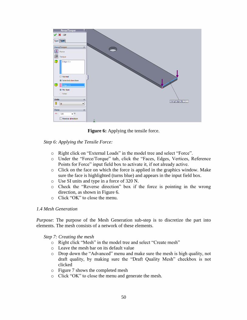
Figure 6: Applying the tensile force.
Step 6: Applying the Tensile Force:
o Right click on “External Loads” in the model tree and select “Force”.
o Under the “Force/Torque” tab, click the “Faces, Edges, Vertices, Reference
Points for Force” input field box to activate it, if not already active.
o Click on the face on which the force is applied in the graphics window. Make
sure the face is highlighted (turns blue) and appears in the input field box.
o Use SI units and type in a force of 320 N.
o Check the “Reverse direction” box if the force is pointing in the wrong
direction, as shown in Figure 6.
o Click “OK” to close the menu.
1.4 Mesh Generation
Purpose: The purpose of the Mesh Generation sub-step is to discretize the part into
elements. The mesh consists of a network of these elements.
Step 7: Creating the mesh
o Right click “Mesh” in the model tree and select “Create mesh”
o Leave the mesh bar on its default value
o Drop down the “Advanced” menu and make sure the mesh is high quality, not
draft quality, by making sure the “Draft Quality Mesh” checkbox is not
clicked
o Figure 7 shows the completed mesh
o Click “OK” to close the menu and generate the mesh.
51
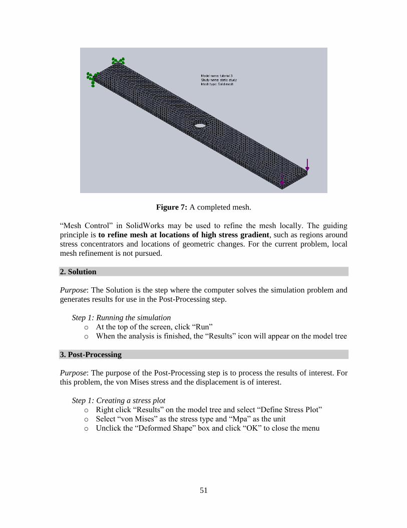
Figure 7: A completed mesh.
“Mesh Control” in SolidWorks may be used to refine the mesh locally. The guiding
principle is to refine mesh at locations of high stress gradient, such as regions around
stress concentrators and locations of geometric changes. For the current problem, local
mesh refinement is not pursued.
2. Solution
Purpose: The Solution is the step where the computer solves the simulation problem and
generates results for use in the Post-Processing step.
Step 1: Running the simulation
o At the top of the screen, click “Run”
o When the analysis is finished, the “Results” icon will appear on the model tree
3. Post-Processing
Purpose: The purpose of the Post-Processing step is to process the results of interest. For
this problem, the von Mises stress and the displacement is of interest.
Step 1: Creating a stress plot
o Right click “Results” on the model tree and select “Define Stress Plot”
o Select “von Mises” as the stress type and “Mpa” as the unit
o Unclick the “Deformed Shape” box and click “OK” to close the menu

52
Figure 8: The von Mises stress plot.
Step 2: Plotting Displacement plot:
o Select the plot for Resultant displacement.
Figure 9: The displacement plot.
Optimization Study:
53
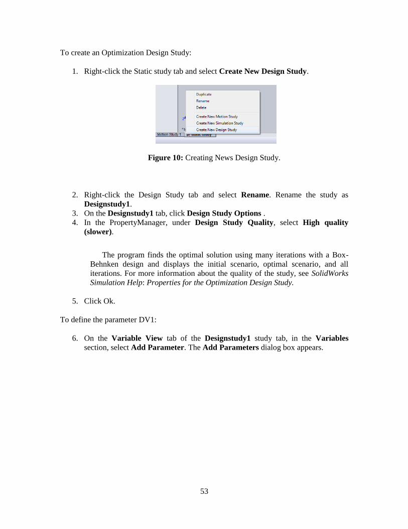
To create an Optimization Design Study:
1. Right-click the Static study tab and select Create New Design Study.
Figure 10: Creating News Design Study.
2. Right-click the Design Study tab and select Rename. Rename the study as
Designstudy1.
3. On the Designstudy1 tab, click Design Study Options .
4. In the PropertyManager, under Design Study Quality, select High quality
(slower).
The program finds the optimal solution using many iterations with a Box-
Behnken design and displays the initial scenario, optimal scenario, and all
iterations. For more information about the quality of the study, see SolidWorks
Simulation Help: Properties for the Optimization Design Study.
5. Click Ok.
To define the parameter DV1:
6. On the Variable View tab of the Designstudy1 study tab, in the Variables
section, select Add Parameter. The Add Parameters dialog box appears.
54
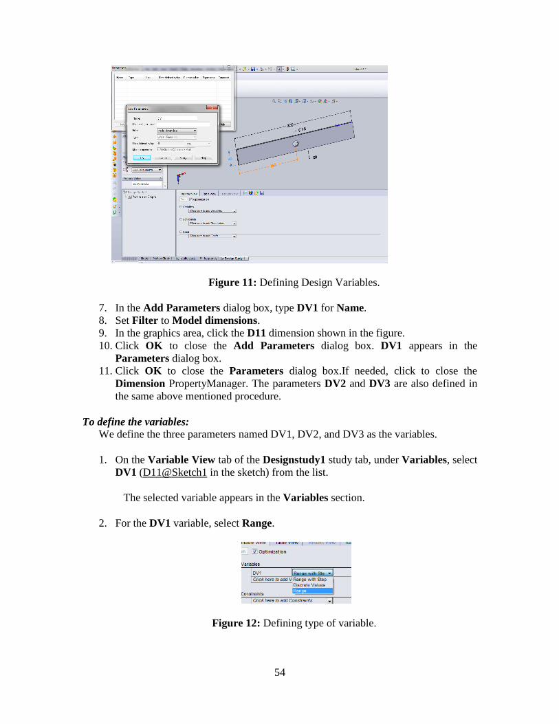
Figure 11: Defining Design Variables.
7. In the Add Parameters dialog box, type DV1 for Name.
8. Set Filter to Model dimensions.
9. In the graphics area, click the D11 dimension shown in the figure.
10. Click OK to close the Add Parameters dialog box. DV1 appears in the
Parameters dialog box.
11. Click OK to close the Parameters dialog box.If needed, click to close the
Dimension PropertyManager. The parameters DV2 and DV3 are also defined in
the same above mentioned procedure.
To define the variables:
We define the three parameters named DV1, DV2, and DV3 as the variables.
1. On the Variable View tab of the Designstudy1 study tab, under Variables, select
DV1 (D11@Sketch1 in the sketch) from the list.
The selected variable appears in the Variables section.
2. For the DV1 variable, select Range.
Figure 12: Defining type of variable.

55
3. The program defines the parameter as a continuous variable for optimization. A
continuous variable is one which can take any value between the limits. For
example, 14.1567mm is a valid value between a minimum value of 45mm and a
maximum value of 55mm.
4. The program varies the model dimension between 25mm and 35mm to find the
optimal value for the variable.
5. Repeat steps 1-3 to add the parameter named DV2 through DV6.
The Variables section lists three design variables.
Figure 13: Defining the Minimum and Maximum values for all DV’s.
We need to define sensors to use them as constraints in a Design Study. The Design
Study runs the corresponding initial Simulation study to update a sensor's value. For
example, it runs the frequency study to track the resonant frequency values.We define a
sensor to track the value of the von Mises stress.
6. On the Variable View tab of the Designstudy1 study tab, in the Constraints
section, select Add Sensor.
7. In the Property Manager, for Sensor Type, select Simulation Data.
8. Under Data Quantity, for Results, select Stress.
9. For component, select VON: von Mises Stress.
10. Under Properties, for Units, select N/mm^2 (MPa) or Psi.
11. For Criterion, select Model Max and click OK.
12. In the Feature Manager Design tree, under Sensors, rename the sensor as Stress1.
13. Similarly the sensor Displacement1 is also defined as like in the tutorial1.
We impose a constraint on the maximum von Mises stress that it should not exceed a
value of 620.4 MPa or 89981 Psi. You can use any sensor or driven global variable to
define constraints for an Optimization Design Study. For more information about
defining sensors as constraints in a Design Study see SolidWorks Simulation Help:
Defining Constraints:
Figure 14: Defining the Maximum value of sensors for constraints.

56
1. On the Designstudy1 Design Study tab, in the Constraints section, make sure
Stress 1 is selected.
The sensor appears in the Constraints section.
2. For Mises, select Is less than.
3. For Max, type 620.4 N/mm^2.
The program automatically selects the Staticstudy study to run and track the
sensor's value since only one static study is defined.
Defining the Displacement constraint:
The maximum resultant displacement should not exceed 0.09812 mm.
4. On the Designstudy1 Design Study tab, in the Constraints section, from the list,
select URES.
The sensor appears in the Constraints section. This pre-defined sensor tracks
the value of resultant displacement.
5. For URES, select Is less than.
6. For Max, type 0.09812 mm.
The program automatically selects the Staticstudy study to run and track the
sensor's value.
Defining a goal:
The objective of this Optimization Design Study is to minimize the volume of the part.
Figure 15: Defining the Goal.
1. On the Designstudy1 Design Study tab, in the Goals section, from the list, select
the Volume1 sensor.
2. The sensor appears in the Goals section.
3. For Volume1, select Minimize.
4. On the Designstudy1 Design Study tab, select Run.

57
Figure 16: Figure showing the run command for iterations.
5. The program runs some iterations (excluding the initial and optimal scenarios)
since you defined a High quality study and three design variables. After running
the experiments, the program calculates the optimal design variables by forming a
response function relating the goal to the variables.
Viewing the Results:
1. Review the Initial column. The column is highlighted in red because the constraints
on von Mises stress and displacement are violated.
2. Review the Optimal column. The column is highlighted in green because
optimization was performed successfully.
Figure 17: Figure showing the iterations.
The program updates the model with the optimal dimensions in the graphics window.
58
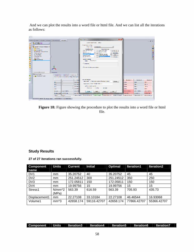
And we can plot the results into a word file or html file. And we can list all the iterations
as follows:
Figure 18: Figure showing the procedure to plot the results into a word file or html
file.
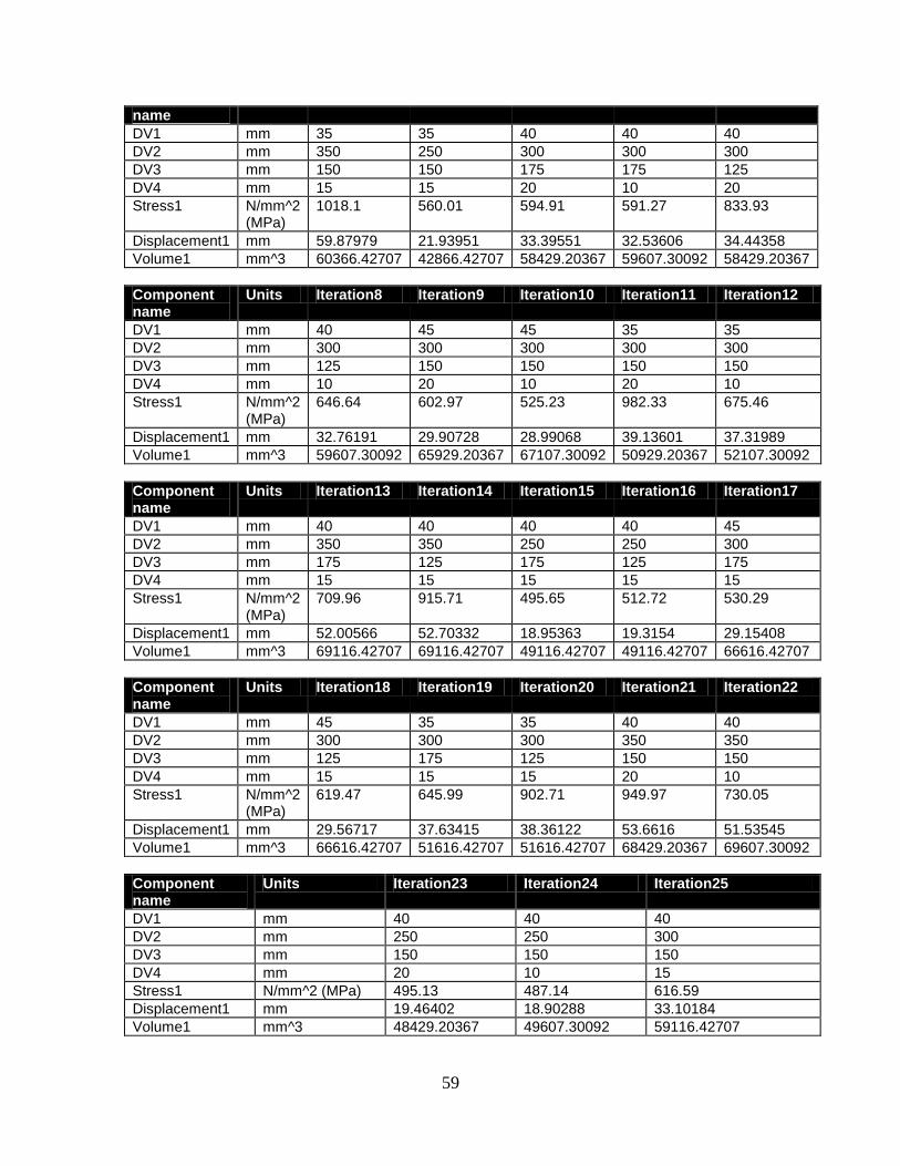
Study Results 27 of 27 iterations ran successfully.
Component name
Units Current Initial Optimal Iteration1 Iteration2
DV1 mm 35.20752 40 35.20752 45 45
DV2 mm 251.24512 300 251.24512 350 250
DV3 mm 172.05811 150 172.05811 150 150
DV4 mm 19.99756 15 19.99756 15 15
Stress1 N/mm^2 (MPa)
563.39 616.59 563.39 705.93 435.73
Displacement1 mm 22.27108 33.10184 22.27108 46.46544 16.93068
Volume1 mm^3 42658.174 59116.42707 42658.174 77866.42707 55366.42707
Component Units Iteration3 Iteration4 Iteration5 Iteration6 Iteration7
59
name
DV1 mm 35 35 40 40 40
DV2 mm 350 250 300 300 300
DV3 mm 150 150 175 175 125
DV4 mm 15 15 20 10 20
Stress1 N/mm^2 (MPa)
1018.1 560.01 594.91 591.27 833.93
Displacement1 mm 59.87979 21.93951 33.39551 32.53606 34.44358
Volume1 mm^3 60366.42707 42866.42707 58429.20367 59607.30092 58429.20367
Component name
Units Iteration8 Iteration9 Iteration10 Iteration11 Iteration12
DV1 mm 40 45 45 35 35
DV2 mm 300 300 300 300 300
DV3 mm 125 150 150 150 150
DV4 mm 10 20 10 20 10
Stress1 N/mm^2 (MPa)
646.64 602.97 525.23 982.33 675.46
Displacement1 mm 32.76191 29.90728 28.99068 39.13601 37.31989
Volume1 mm^3 59607.30092 65929.20367 67107.30092 50929.20367 52107.30092
Component name
Units Iteration13 Iteration14 Iteration15 Iteration16 Iteration17
DV1 mm 40 40 40 40 45
DV2 mm 350 350 250 250 300
DV3 mm 175 125 175 125 175
DV4 mm 15 15 15 15 15
Stress1 N/mm^2 (MPa)
709.96 915.71 495.65 512.72 530.29
Displacement1 mm 52.00566 52.70332 18.95363 19.3154 29.15408
Volume1 mm^3 69116.42707 69116.42707 49116.42707 49116.42707 66616.42707
Component name
Units Iteration18 Iteration19 Iteration20 Iteration21 Iteration22
DV1 mm 45 35 35 40 40
DV2 mm 300 300 300 350 350
DV3 mm 125 175 125 150 150
DV4 mm 15 15 15 20 10
Stress1 N/mm^2 (MPa)
619.47 645.99 902.71 949.97 730.05
Displacement1 mm 29.56717 37.63415 38.36122 53.6616 51.53545
Volume1 mm^3 66616.42707 51616.42707 51616.42707 68429.20367 69607.30092
Component name
Units Iteration23 Iteration24 Iteration25
DV1 mm 40 40 40
DV2 mm 250 250 300
DV3 mm 150 150 150
DV4 mm 20 10 15
Stress1 N/mm^2 (MPa) 495.13 487.14 616.59
Displacement1 mm 19.46402 18.90288 33.10184
Volume1 mm^3 48429.20367 49607.30092 59116.42707

60
Attachment E. Post-test
1. The internal force per unit area acting inside the body when a force is applied on
the body is called:
O Stress
O Strain
O Displacement
O Other
2. What is state variable?
3. Define basic and feasible design space
4. What is an Optimum Design?
5. Ranges and limits are set for which entity in an optimization study?
O goals
O Constraints
O both the above
O None of the above
6. Bending moment induces:
O Tensile stress
O Compressive stress
O Both tensile and compressive stress
O Shear stress
7. State variables can be directly controlled.
O True
O False
8. A point in the feasible design space represents one feasible design
61
O True
O False
9. What is Young’s modulus?
O The ratio of the normal stress to the normal strain
O The ratio of the shear stress to the normal stress
O The ratio of the displacement to the normal stress
O The ratio of shear stress to shear strain
10. The 2D space in which the horizontal dimension represents all feasible designs and
the vertical dimension represents the objective function is:
O Feasible design space
O Evaluation space
O All the above
O None of the above

62
Attachment F. Assessment
Do you feel it was bad to not have a teacher there to answer any questions you
might have?
O It didn’t matter
O It would have been nice
O I really wanted to ask a question
How did the interactivity of the program affect your learning?
O Improved it a lot
O Improved it some
O No difference
O Hurt it some
O Hurt it a lot
The six levels of Bloom’s Taxonomy are listed below. Rank how well this
learning module covers each level. 5 meaning exceptionally well and 1
meaning very poor.
1. Knowledge (remembering previously learned material)
O 5
O 4
O 3
O 2
O 1
2. Comprehension (the ability to grasp the meaning of the material and give
examples)
O 5
O 4
O 3
O 2
O 1
3. Application (the ability to use the material in new situations)
O 5
O 4
O 3
O 2
O 1
63
4. Analysis (the ability to break down material into its component parts so that
its organizational structure may be understood)
O 5
O 4
O 3
O 2
O 1
5. Synthesis (the ability to put parts together to form a new whole)
O 5
O 4
O 3
O 2
O 1
6. Evaluation (the ability to judge the value of the material for a given purpose)
O 5
O 4
O 3
O 2
O 1
Do you think the mixed text and video format works well?
O Yes
O Indifferent
O No
Do you think the module presents an affective method of learning FEA?
O Yes
O Indifferent
O No
Did you prefer this module over the traditional classroom learning
experience? Why or why not.

64
How accurate would it be to call this module self-contained and stand-alone?
O Very accurate
O Accurate
O Indifferent
O Inaccurate
O Very inaccurate
What specifically did you like and/or dislike about the module.
How useful were the practice problems?
O Very helpful
O Helpful
O Indifferent
O Unhelpful
O Very unhelpful
Was there any part of the module that you felt was unnecessary of redundant?
Was there a need for any additional parts?
Please list any suggestions for improving this module.
Overall, how would you rate your experience taking this module?
O Excellent
O Fair
O Average
O Poor
O Awful
65
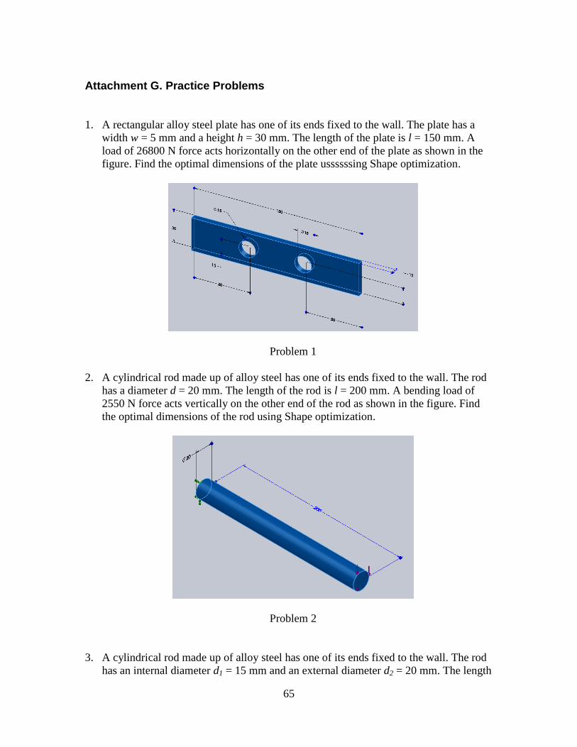
Attachment G. Practice Problems
1. A rectangular alloy steel plate has one of its ends fixed to the wall. The plate has a
width w = 5 mm and a height h = 30 mm. The length of the plate is l = 150 mm. A
load of 26800 N force acts horizontally on the other end of the plate as shown in the
figure. Find the optimal dimensions of the plate ussssssing Shape optimization.
Problem 1
2. A cylindrical rod made up of alloy steel has one of its ends fixed to the wall. The rod
has a diameter d = 20 mm. The length of the rod is l = 200 mm. A bending load of
2550 N force acts vertically on the other end of the rod as shown in the figure. Find
the optimal dimensions of the rod using Shape optimization.
Problem 2
3. A cylindrical rod made up of alloy steel has one of its ends fixed to the wall. The rod
has an internal diameter d1 = 15 mm and an external diameter d2 = 20 mm. The length
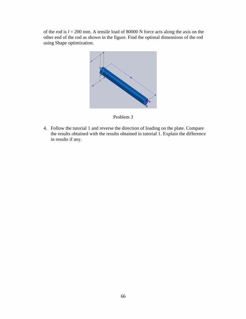
66
of the rod is l = 200 mm. A tensile load of 80000 N force acts along the axis on the
other end of the rod as shown in the figure. Find the optimal dimensions of the rod
using Shape optimization.
Problem 3
4. Follow the tutorial 1 and reverse the direction of loading on the plate. Compare
the results obtained with the results obtained in tutorial 1. Explain the difference
in results if any.