Learning in Real Time: Theory and Empirical Evidence from ...

Learning in Real Time:Theory and Empirical Evidence from theTerm Structure of Survey Forecasts

Andrew Patton and Allan Timmermann

Oxford and UC-San Diego

November 2007

Patton & Timmermann (Oxford and UC-San Diego) Learning in Real Time November 2007 1 / 55

Motivation

Uncertainty about macroeconomic variables such as GDP growth andin�ation enters into the decision-making processes of governments,�rms and individuals.

welfare implications of macroeconomic volatility, see Ramey and Ramey(1995, AER)

irreversibility and lags in investment decisions, see Kydland andPrescott (1982, Econometrica)

determination of asset prices, see Andersen et al. (2003, AER)

volatility and volume in asset markets, see Beber and Brandt (2006)

responsiveness of investment to information, see Bloom et al. (2007,REStud)

Contributions of this paper

1 We use a rich data set containing survey forecasts of annual GDPgrowth and in�ation, with forecast horizons ranging from 1 to 24months, to shed light on:

1 How quickly agents learn about these GDP growth and in�ation

2 What factors a¤ect the accuracy of their forecasts

3 What factors might be behind the observed amount of disagreementbetween individual forecasters

2 We analyse this data via a simple but �exible theoretical frameworkfor studying panels of forecasts containing multiple horizons.

1 This framework is designed to model both the consensus forecast andthe dispersion amongst forecasts, across many horizons.

Detailed description of the data

We have T = 14 years of data (1991-2004) from ConsensusEconomics for real GDP growth and CPI in�ation.

In each year we have forecasts for H = 24 di¤erent forecast horizons.

We have consensus forecasts and the cross-sectional dispersion ofindividual forecasts, but not the individual forecasts themselves.

The realization of the target variable is the value reported by the IMFin the September of the following year.

Our measure of the target variable may be subject to measurementerror - we do not explicitly model this.

Sample root mean squared errors as a function of theforecast horizon: GDP growth

24 21 18 15 12 9 6 3 00

0.2

0.4

0.6

0.8

1

1.2

1.4

1.6

horizon

RM

SE

Sample RMSE for US forecasts

GDP growth

Sample root mean squared errors as a function of theforecast horizon: GDP growth and In�ation

24 21 18 15 12 9 6 3 10

0.2

0.4

0.6

0.8

1

1.2

1.4

1.6

horizon

RM

SE

Sample RMSE for US forecasts

GDP growthInflation

Cross-sectional forecast dispersion as a function of theforecast horizon: GDP growth

24 21 18 15 12 9 6 3 00

0.05

0.1

0.15

0.2

0.25

0.3

0.35

0.4

0.45

0.5

horizon

disp

ersi

onSample forecast dispersion for US forecasts

GDP growth

Cross-sectional forecast dispersion as a function of theforecast horizon: GDP growth and In�ation

24 21 18 15 12 9 6 3 00

0.05

0.1

0.15

0.2

0.25

0.3

0.35

0.4

0.45

0.5

horizon

disp

ersi


GDP growthInflation

Outline of the talk

1 Introduction and brief description of the data

2 A theoretical model for the term structure of RMSE

1 Theoretical predictions

2 Estimation by generalised method of moments

3 Estimating the persistent components from GDP growth and in�ationfrom the survey forecasts

3 A theoretical model for the term structure of forecast dispersion


2 Joint estimation by simulated method of moments

3 A simple model for time-varying dispersion

4 Summary and conclusions

First: Are the survey forecasts unbiased?

Our use of the Consensus Economics survey forecasts in this studyrelies on the assumption that

zt ,t�h = E�zt jFt�h

�i.e., that the forecasts are optimal under quadratic loss,L (z , z) = (z � z)2

We ran a battery of tests of forecast optimality: testing for bias,Mincer-Zarnowitz regressions, and testing for weakly increasing MSEas a function of the forecast horizon.

Almost all of these tests failed to reject the null of optimality(unsurprising with T = 14) and so we proceed as though thecondition is satis�ed.

Bias and MZ tests of the consensus forecast

Bias MZ p-valuesHorizon GDP growth In�ation GDP growth In�ation1 0.11 0.01 0.99 1.002 0.07 0.02 0.99 1.003 0.03 0.04�� 0.99 1.006 0.05 0.08� 0.99 1.009 -0.06 0.01 0.98 0.9912 -0.34 0.03 0.95 0.9618 -0.06 0.29 0.99 0.9824 -0.09 0.37� 0.98 0.98

Learning and uncertainty in our model

We assume that forecasters know the DGP and its parameters, thusruling out estimation error and learning as sources of forecast errorsand dispersion.

The primary source of uncertainty in the model concerns the futurevalue of the variable of interest

When we extend to allow for measurement error, uncertainty exists alsofor current and past values of the variable of interest

Modelling the forecasters�learning about the DGP and/or itsparameters requires a long time series, whereas our sample is justT = 14 years.

Notation

yt : monthly value of variable of interest

zt =11

∑j=0yt�j : annual value of variable of interest

zt ,t�h : the consensus forecast of zt made at time t � h

Ft�h : information available at time t � h

et ,t�h = zt � zt ,t�h : consensus forecast error

The benchmark model

zt =11

∑j=0yt�j

yt = xt + utxt = φxt�1 + εt , jφj < 1

�utεt

�s iid

�0,�

σ2u 00 σ2ε

��zt ,t�h = E [zt jFt�h ]Ft�h = σ

�fxs ,ysgt�hs=1

�

Optimal forecasts and MSE term structures

Prop 1 (ii): The mean squared error of the optimal forecast as a functionof the forecast horizon is:

E�e2t ,t�h

�=

8>>>>>>>>>><>>>>>>>>>>:

hσ2u +1

(1�φ)2

�h� 2φ(1�φh)

1�φ +φ2(1�φ2h)1�φ2

�σ2ε ,

for 1 � h < 12

12σ2u +1

(1�φ)2

�12� 2φ(1�φ12)

1�φ +φ2(1�φ24)1�φ2

�σ2ε

+φ2(1�φ12)

2(1�φ2h�24)

(1�φ)3(1+φ)σ2ε , for h � 12

RMSE term structures under the benchmark model, forvarious levels of persistence.

24 21 18 15 12 9 6 3 00

0.2

0.4

0.6

0.8

1

1.2

1.4

1.6

forecast horizon

RM

SERMSE for various persistence parameters

phi= 0phi= 0.5phi=0.75phi= 0.9phi=0.95

Figure:

Measurement errors - a Kalman �lter approach

Our benchmark model assumed that both the predictable andunpredictable components of the target variable are perfectly observedby the forecasters.

This implies that the squared forecast errors converge to zero as thehorizon shrinks - this does not match the data.

We need to extend the model to allow for imperfect observation ofthe variable(s) of interest.

A more realistic framework would allow both components to bemeasured with noise. We use the Kalman �lter to handle such anapproach.

A state-space model

The state equation for this model is unchanged:�1 �10 1

� �ytxt

�=

�0 00 φ

� �yt�1xt�1

�+

�utεt

��utεt

�s iid

�0,�

σ2u 00 σ2ε

��The measurement equation is assumed to be:�

ytxt

�=

�ytxt

�+

�ηtψt

��

ηtψt

�s iid

�0,�

σ2η 00 σ2ψ

��This is a standard state-space form and can be studied using textbookmethods (see Harvey 1989 or Hamilton 1994).

Term structure of RMSE for various measurement errors

The mean squared error of the optimal forecast in this state-spaceframework can be obtained analytically:

For h � 12 it is simply a function of the forecast errors for horizons ofdi¤erent lengths

For h < 12 it is a (complicated) function of forecast, �nowcast�and�backcast� errors

While these expressions can be obtained in closed-form, they are hardto interpret directly (see technical appendix of the paper)

Term structure of RMSE for various measurement errorsSig-psi = +in�nity, sig-eta = k*sig-u for various k

24 21 18 15 12 9 6 3 10

0.2

0.4

0.6

0.8

1

1.2

1.4

1.6

forecast horizon

RM

SE

RMSE for various measurement error variance parameters

k=0.01k= 0.5k= 1k= 2k= 3k= 5k= 10

Figure:

Estimation method

Our vector of unknown parameters for the model of the �termstructure�of mean squared consensus errors isθ =

�σu , σε, φ, ση, σψ

�0.

We estimate these parameters by GMM:

θT � argminθ2Θ

gT (θ)0WT gT (θ)

where gT (θ) � 1T

T

∑t=1

264 e2t ,t�1 �MSE1 (θ)...

e2t ,t�24 �MSE24 (θ)

375where MSEh (θ) is the model-implied mean-squared error for horizonh.

Estimation method - details

The weight matrix used is the identity matrix: less e¢ cient, butmaintains focus on the entire term structure.

The model-implied covariance matrix of the moments, obtained viasimulation of 10,000 non-overlapping years of data, is used tocompute standard errors and the test of over-identifying restrictions.

After some experimentation we �xed ση = 2σu and set σψ ! ∞ toimprove the identi�cation of the model.

We initially used all 24 horizons for estimation, but in light of�nite-sample studies of GMM estimators, we settled on estimating themodel with just six forecast horizons: h = 1, 3, 6, 12, 18, 24.

GMM parameter estimates: consensus model

σu σε φ J p-val

GDP growth 0.06(0.01)

0.05(0.01)

0.94(0.03)

0.40

In�ation 0.00(��)

0.02(0.01)

0.95(0.05)

0.94

Term structures of RMSE for GDP growth and in�ation.

24 21 18 15 12 9 6 3 10

0.2

0.4

0.6

0.8

1

1.2

1.4

1.6

horizon

RM

SE

US GDP growth

24 21 18 15 12 9 6 3 10

0.2

0.4

0.6

0.8

1

1.2

1.4

1.6

RM

SE

horizon

US Inflation

sample RMSEmodel no measurement errormodel Kalman filter

Term structures of R2 for GDP growth and in�ation.

24 21 18 15 12 9 6 3 10

0.2

0.4

0.6

0.8

1

R2

US GDP growth

24 21 18 15 12 9 6 3 10

0.2

0.4

0.6

0.8

1

horizon

R2

US Inflation

sample R 2

model no measurement errormodel Kalman filter

Extracting the components of GDP and In�ation

Our simple framework for the monthly data generating process:

ξt ��ytxt

�=

�0 φ0 φ

�| {z }

�F

�yt�1xt�1

�+

�ut + εt

εt

�

wt �11

∑j=0

ξt�j =

266411∑j=0yt�j

11∑j=0xt�j

3775

Extracting the components of GDP and In�ation

Optimal forecasts in this case are:

E�wt jFt�h

�=

11

∑j=0F h�j

!E�ξt�h jFt�h

�, h � 12

E�wt jFt�h

�=

11

∑j=h+1

E�ξt�j jFt�h

�+

h

∑j=0F h�j

!E�ξt�h jFt�h

�,

So optimal forecasts are a function of the �nowcast� and �backcast�values of wt . Given an estimate of the parameters de�ning the DGP, itis possible to extract �ltered and smoothed estimates of the persistent(xt ) and transitory (ut ) components of the variable of interest.

Forecasters�implied persistent component of GDP growthRecall y[t] = x[t] + u[t] ( total = persistent + transitory )

Jan91 Jan93 Jan95 Jan97 Jan99 Jan01 Jan03 Dec042

1

0

1

2

3

4

5

6

Per

cent

(ann

ualis

ed)

GDP growth

actualxhat filteredxhat smoothed

Forecasters�implied persistent component of In�ationRecall y[t] = x[t] + u[t] ( total = persistent + transitory )

Jan91 Jan93 Jan95 Jan97 Jan99 Jan01 Jan03 Dec041

2

3

4

5

6

7

Per

cent

(ann

ualis

ed)

Inflation

actualxhat fil teredxhat smoothed

Summary of �ndings for the RMSE term structure

A simple model based on a persistent and a transitory decompositionof the target variable �ts the data well

1 A simple AR(1) model for the persistent component was su¢ cient,though our framework could be extended to handle more generalAR(p) or multiple component AR(pi ) models

2 Allowing for measurement error is important for GDP growth, thoughnot for in�ation. This is consistent with the �real time data� literaturein macroeconomics, see Croushore and Stark (2001) for example.

3 No �seasonal� component was needed (quarterly releases of �gures,monthly announcements, etc): information appears to be smoothlyincorporated into consensus forecasts.

Outline of the talk

1 Introduction and brief description of the data

2 A theoretical model for the term structure of RMSE


2 Estimation by generalised method of moments

3 Estimating the persistent components from GDP growth and in�ationfrom the survey forecasts

3 A theoretical model for the term structure of forecast dispersion


2 Joint estimation by simulated method of moments

3 A simple model for time-varying dispersion

4 Summary and conclusions

Dispersion among forecasters

Our second variable of interest is the degree to which agents disagreeabout the expected value of the target variable. We measure this by

d2t ,t�h � 1Nt ,t�h

Nt ,t�h

∑i=1

(zi ,t ,t�h � zt ,t�h)2

Cross-sectional forecast dispersion as a function of theforecast horizon: GDP growth and In�ation

24 21 18 15 12 9 6 3 00

0.05

0.1

0.15

0.2

0.25

0.3

0.35

0.4

0.45

0.5

horizon

disp

ersi


GDP growthInflation

A model for dispersion

The �rst source of dispersion is di¤erences in signals:

yi ,t = yt + ηt + νi ,t�ηtνt

�s iid

�0,�

σ2η 00 σ2ν

��But as the forecast survey results are published (with a lag) we alsoassume that the forecaster�s time t information set includes:

yt�1 = yt�1 + ηt�1

From these two measurement variables, the individual forecastercomputes the optimal forecast using the Kalman �lter:

z�i ,t ,t�h � E�zt jFi ,t�h

�

Di¤erences in signals & dispersion as h grows

Allowing for di¤erences in signals is a natural starting point forcapturing dispersion, but it has an important counter-factualimplication:

As h! ∞, the value of any signal for predicting the target variablegoes to zero, and so all forecasts converge to the unconditional mean:

z�i ,t ,t�h � E�zt jFi ,t�h

�! E [zt ] as h! ∞

so d2t ,t�h � 1Nt ,t�h

Nt ,t�h

∑i=1

(zi ,t ,t�h � zt ,t�h)2 ! 0 as h! ∞

Yet we saw that d2t ,t�h ! δ > 0 as h! ∞ for both variables in oursample. So there must be another source of dispersion.

Di¤erences in beliefs about long-run values

One simple way of allowing for dispersion at long horizons is to allowthe forecasters to have di¤ering beliefs about the long-run averagevalues of GDP growth and in�ation.

This approach is a special case of allowing for di¤erent subjectiveprobability densities across forecasters, see Pesaran and Weale (2005).

These di¤erences can be motivated in a number of ways:

Di¤erent models for equilibrium rates of GDP growth and in�ation

Di¤erent samples of data, based on di¤erent beliefs about previousstructural breaks, etc.

Di¤erent Bayesian priors, which a¤ect the forecasts issued.

The outcome of a �game�played between forecasters, see Laster, et al.(1999) or Ottaviani and Sørensen (2006) for example

A model for di¤erences in beliefs

Forecaster i�s prior belief about the average value of zt is denoted µi .

We assume that forecaster i �shrinks� the Kalman �lter forecasttowards his prior belief about the unconditional mean of zt . Thedegree of shrinkage is governed by the parameter κ2 � 0

zi ,t�h,t = ωhµi + (1�ωh)E�zt jFi ,t�h

�where ωh =

E�e�2i ,t ,t�h

�κ2 + E

he�2i ,t ,t�h

ie�i ,t�h,t � zt � E

�zt jFi ,t�h

�

The degree of �shrinkage�

The weights, ωh, placed on the prior vary across h in a mannerconsistent with standard forecast combinations: as the Kalman �lterforecast becomes more accurate the weight attached to that forecastincreases.

For short horizons, h! 0, the weight attached to the prior falls,while for long horizons the weight attached to the prior grows.

For analytical tractability, and for better �nite sample identi�cation ofκ2, we impose that κ2 is constant across all forecasters.

Model-implied dispersion

We normalise µ = 0 since we cannot separately identify µ and σ2µfrom our data. This is reasonable if the number of �optimistic�forecasters is approximately equal to the number of �pessimistic�forecasters.

Our model for dispersion is the unconditional expectation of d2t ,t�h.We allow for a heteroskedastic residual term for our model ofdispersion, with variance related to the level of the dispersion.

d2t ,t�h = δ2h (θ) � λt ,t�h

where δ2h (θ) � E�d2t ,t�h

�E [λt ,t�h ] = 1

V [λt ,t�h ] = σ2λ.

Model-implied dispersion as a function of Sig-muWith Sig-nu=2*Sig-u, kappa=0.5*Sig-z, Sig-eta = 2*Sig-u.

24 21 18 15 12 9 6 3 10

0.2

0.4

0.6

0.8

1

horizon

disp

ersi

onDispersion for various values of sigmu

sigmu= 1.5sigmu= 1sigmu=0.75sigmu= 0.5sigmu=0.25

Estimation method

Our vector of parameters for the model of the mean squaredconsensus errors and dispersion is θ =

�σu , σε, φ, σν, σµ, κ, σλ

�0. We

estimate these parameters by SMM:

θT � argminθ2Θ

gT (θ)0WT gT (θ)

where gT (θ) � 1T

T

∑t=1

26666666664

e2t ,t�1 �MSE1 (θ)...

d2t ,t�1 � δ21 (θ)...�

d2t ,t�1 � δ21 (θ)�2 � σ2δ,h (θ)

...

37777777775where MSEh (θ), δ2h (θ) and σ2δ,h (θ) are the model-implied MSE,dispersion, and dispersion variance.

Estimation method - details

The value of δ2h (θ) cannot be obtained in closed-form; we simulateN = 30 individual forecasters for T = 600 months of non-overlappingdata.

The weight matrix used is again the identity matrix, so all horizons ofRMSE and dispersion (and dispersion variance) get equal weight inthe estimation.

Standard errors and the test of over-identifying restrictions are againbased on the model-implied covariance matrix of the moments.

We again estimated the model with just six forecast horizons:h = 1, 3, 6, 12, 18, 24.

GMM parameter estimates: consensus and dispersionmodel

σu σε φ σν σµ κ J p-val


0.05(0.01)

0.94(0.03)

0.69(1.00)

0.67(0.39)

1.41(0.94)

0.86


0.02(0.01)

0.95(0.05)

0.05(0.17)

0.51(0.13)

0.49(0.17)

0.00

Term structures of dispersion for GDP growth and in�ationin the US.

24 21 18 15 12 9 6 3 10

0.1

0.2

0.3

0.4

0.5

horizon

disp

ersi

on

US GDP growth

24 21 18 15 12 9 6 3 10

0.1

0.2

0.3

0.4

0.5

disp

ersi

on

horizon

US Inflation

sample dispersionmodel no diffs in signalmodel Kalman filter

Interpreting the results from the dispersion model

The model for in�ation dispersion �ts well for h � 12, but for shorthorizons it systematically under-estimates dispersion

why is observed in�ation dispersion is so high at short horizons?

GDP growth In�ation

h RMSE DISP ratio RMSE DISP ratio1 0.56 0.08 0.15 0.05 0.07 1.453 0.61 0.14 0.23 0.08 0.11 1.296 0.67 0.21 0.31 0.17 0.16 0.9112 1.18 0.41 0.35 0.47 0.33 0.7024 1.52 0.48 0.32 0.74 0.45 0.60

A model for time-varying dispersion

There is a growing body of empirical and theoretical work on therelationship between uncertainty (somehow de�ned) and theeconomic environment.

We use the default spread on corporate bonds for this purpose - thisis known to be a strongly counter-cyclical variable.

We model increased uncertainty as an increase in the di¤erences inbeliefs about long-run values

log σ2µ,t = βµ0 + β

µ1 log St

A positive coe¢ cient on log St will imply that higher default spreadscoincide with greater disagreement about long-run values of theseries, generating higher dispersion.

GMM parameter estimates: consensus and time-varyingdispersion model

σu σε φ σν κ βµ0 β

µ1 J p-val


0.05(0.01)

0.94(0.03)

0.69(0.87)

1.41(0.74)

-0.56(1.10)

3.08(1.83)

0.91


0.02(0.01)

0.95(0.05)

0.05(0.17)

0.49(0.17)

-1.32(0.55)

0.18(2.37)

0.00

Term structures of dispersion for GDP growth and in�ationin the US.Conditional on the level of the default spread

24 21 18 15 12 9 6 3 10

0.1

0.2

0.3

0.4

0.5

0.6

0.7

0.8

0.9

1

horizon

disp

ers

ion

(st

d de

v)

GDP growth forecasts

24 21 18 15 12 9 6 3 10

0.05

0.1

0.15

0.2

0.25

0.3

0.35

0.4

0.45

0.5

horizon

Inflation forecas ts

sample dispers ionmodel dispers ion, high defsprmodel dispers ion, avg defsprmodel dispers ion, low defspr

Summary of results: the RMSE term structure

Main �nding: A simple model of GDP and in�ation dynamics issu¢ cient to accurately describe the complete term structure ofconsensus mean squared forecast errors.

The estimated persistence parameters are consistent with estimatesobtained using lower-frequency data.

Measurement error is an important part of the model for GDP growth,though not for in�ation

The forecasters in this panel appear to have taken several years toadjust their forecasts to re�ect the higher GDP growth and lowerin�ation �gures during the 1990s

Summary of results: the dispersion term structure

Di¤erences in prior beliefs about long-run averages explain almost allof the observed dispersion for both GDP growth and in�ationforecasts.

Important di¤erences in the properties of forecast dispersion for thesetwo variables emerged:

The GDP forecast dispersion �t the data well, while the in�ationdispersion model failed at short horizons

In�ation dispersion is high relative to the RMSE of the consensusforecast, while GDP dispersion is only a fraction of the RMSE

Dispersion in GDP forecasts varies counter-cyclically in a signi�cantfashion, while in�ation forecast dispersion appears unrelated to thebusiness cycle

Extensions

1 Formally model learning by forecasters: allow them to updateestimates of parameters rather than assume them known.

2 Consider the impact of other non-stationarities in the data: structuralbreaks in GDP variance or the level of in�ation, for example.

3 Combine our panel of forecasts with samples of data on the targetvariables over a longer sample but at a lower frequency.

The form of the target variable

Our analysis in the previous sections take the target variable, zt , asthe December-on-December change in the log-level of US real GDPor the Consumer Price Index

In the Consensus Economics survey, however, the target variables arede�ned as:

zGDPt � PtPt�1

� 1

z INFt � P t

P t�1� 1,

where Pt � 14

3

∑j=0PGDPt�3j , and P t �

112

11

∑j=0P INFt�j

The form of the target variable, cont�d

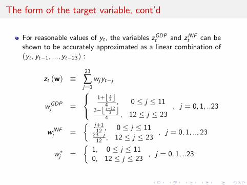
For reasonable values of yt , the variables zGDPt and z INFt can beshown to be accurately approximated as a linear combination of(yt , yt�1, ..., yt�23) :

zt (w) �23

∑j=0wjyt�j

wGDPj =

8<:1+b j3 c4 , 0 � j � 11

3�b j�123 c4 , 12 � j � 23

, j = 0, 1, ..23

w INFj =

� j+112 , 0 � j � 1123�j12 , 12 � j � 23 , j = 0, 1, .., 23

w �j =

�1, 0 � j � 110, 12 � j � 23 , j = 0, 1, ..23

The weights for GDP growth

JanY1MarY1 JunY1 SepY1 DecY1JanY2MarY2 JunY2 SepY2 DecY20.2

0

0.2

0.4

0.6

0.8

1

k

wei

ght o

n y[

tk]

linear combination of monthly changes in loglevel of index, quarterly averaging

analytical approximationoptimal OLS approximation

The weights for in�ation

JanY1MarY1 JunY1 SepY1 DecY1JanY2MarY2 JunY2 SepY2 DecY20.2

0

0.2

0.4

0.6

0.8

1

k

wei

ght o

n y[

tk]

linear combination of monthly changes in loglevel of index

analytical approximationoptimal OLS approximation

Learning in Real Time: Theory and Empirical Evidence from ...

Documents

Transcript of Learning in Real Time: Theory and Empirical Evidence from ...