Learning in Implicit Generative Models

Shakir Mohamed 1 Balaji Lakshminarayanan 1

Abstract

Generative adversarial networks (GANs) providean algorithmic framework for constructing gen-erative models with several appealing proper-ties: they do not require a likelihood functionto be specified, only a generating procedure; theyprovide samples that are sharp and compelling;and they allow us to harness our knowledge ofbuilding highly accurate neural network classi-fiers. Here, we develop our understanding ofGANs with the aim of forming a rich view ofthis growing area of machine learning—to buildconnections to the diverse set of statistical think-ing on this topic, of which much can be gainedby a mutual exchange of ideas. We frame GANswithin the wider landscape of algorithms for learn-ing in implicit generative models—models thatonly specify a stochastic procedure with whichto generate data—and relate these ideas to mod-elling problems in related fields, such as econo-metrics and approximate Bayesian computation.We develop likelihood-free inference methodsand highlight hypothesis testing as a principlefor learning in implicit generative models, usingwhich we are able to derive the objective func-tion used by GANs, and many other related ob-jectives. The testing viewpoint directs our fo-cus to the general problem of density-ratio anddensity-difference estimation. There are four ap-proaches for density comparison, one of whichis a solution using classifiers to distinguish realfrom generated data. Other approaches such asdivergence minimisation and moment matchinghave also been explored, and we synthesise theseviews to form an understanding in terms of the re-lationships between them and the wider literature,highlighting avenues for future exploration andcross-pollination.

*Equal contribution 1DeepMind, London, UK. Correspondenceto: Shakir Mohamed <shakir@google.com>, Balaji Lakshmi-narayanan <balajiln@google.com>.

1. Implicit Generative ModelsIt is useful to make a distinction between two types of prob-abilistic models: prescribed and implicit models (Diggleand Gratton, 1984). Prescribed probabilistic models arethose that provide an explicit parametric specification of thedistribution of an observed random variable x, specifying alog-likelihood function log qθ(x) with parameters θ. Mostmodels in machine learning and statistics are of this form,whether they be state-of-the-art classifiers for object recog-nition, complex sequence models for machine translation,or fine-grained spatio-temporal models tracking the spreadof disease. Alternatively, we can specify implicit probabilis-tic models that define a stochastic procedure that directlygenerates data. Such models are the natural approach forproblems in climate and weather, population genetics, andecology, since the mechanistic understanding of such sys-tems can be used to directly create a data simulator, andhence the model. It is exactly because implicit models aremore natural for many problems that they are of interest andimportance.

Implicit generative models use a latent variable z and trans-form it using a deterministic function Gθ that maps fromRm → Rd using parameters θ. Such models are amongstthe most fundamental of models, e.g., many of the basicmethods for generating non-uniform random variates arebased on simple implicit models and one-line transforma-tions (Devroye, 2006). In general, implicit generative mod-els specify a valid density on the output space that forms aneffective likelihood function:

x = Gθ(z′); z′ ∼ q(z) (1)

qθ(x) =∂

∂x1. . .

∂

∂xd

∫{Gθ(z)≤x}

q(z)dz, (2)

where q(z) is a latent variable that provides the externalsource of randomness and equation (2) is the definition ofthe transformed density as the derivative of the cumulativedistribution function. When the function G is well-defined,such as when the function is invertible, or has dimensionsm = d with easily characterised roots, we recover the fa-miliar rule for transformations of probability distributions.We are interested in developing more general and flexibleimplicit generative models where the function G is a non-linear function with d > m, specified by deep networks.

arX

iv:1

610.

0348

3v4

[st

at.M

L]

27

Feb

2017

Learning in Implicit Generative Models

The integral (2) is intractable in this case: we will be unableto determine the set {Gθ(z) ≤ x}, the integral will often beunknown even when the integration regions are known and,the derivative is high-dimensional and difficult to compute.Intractability is also a challenge for prescribed models, butthe lack of a likelihood term significantly reduces the toolsavailable for learning. In implicit models, this difficulty mo-tivates the need for methods that side-step the intractabilityof the likelihood (2), or are likelihood-free.

Both generative adversarial networks (GANs) (Goodfellowet al., 2014) and classifier ABC (Gutmann et al., 2014)provide a solution for exactly this type of problem. Theseapproaches specify algorithmic frameworks for learningin implicit generative models, also referred to as genera-tor networks, generative neural samplers or (differentiable)simulator-models. Both approaches rely on a learning princi-ple based on discriminating real from generated data, whichwe shall show instantiates a core principle of likelihood-freeinference, that of hypothesis and two-sample testing. Manyof the methods we discuss are known in isolation, spreaddisparately throughout the literature. Our core contributionis to make explicit their probabilistic basis and to clearlydiscuss the connections between them.

Note on notation. We denote data by the random variable x,the (unknown) true data density by p∗(x), our (intractable)model density by qθ(x). q(z) is a density over latent vari-ables z. Parameters of the model are θ, and parameters ofthe ratio and discriminator functions are φ.

2. Hypothesis Testing and Density Ratios2.1. Likelihood-free Inference

Without a likelihood function, many of the widely-usedtools for inference and parameter learning become unavail-able. But there are tools that remain, including the method-of-moments (Hall, 2005), the empirical likelihood (Owen,1988), Monte Carlo sampling (Marin et al., 2012), and mean-shift estimation (Fukunaga and Hostetler, 1975). Since wecan easily draw samples from the model, we can use anymethod that compares two sets of samples—one from thetrue data distribution and one from the model distribution—to drive learning. This is a process of density estimation-by-comparison, comprising two steps: comparison and es-timation. For comparison, we test the hypothesis that thetrue data distribution p∗(x) and our model distribution q(x)are equal, using the density difference r(x) = p∗(x)− q(x),or the density ratio r(x) = p∗(x)/q(x). The comparator r(x)provides information about the departure of our model dis-tribution from the true distribution and can be motivatedby either the Neyman-Pearson lemma or the Bayesian pos-terior evidence, appearing in the likelihood ratio and theBayes factor (Kass and Raftery, 1995). For estimation, we

use information from the comparison to drive learning ofthe parameters of the generative model. This is the focusof our approach for likelihood-free inference: estimatingdensity-comparisons and using them as the driving principlefor learning in implicit generative models.

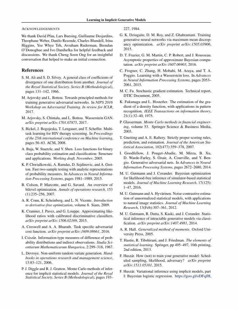
The direct approach of comparing distributions by first com-puting the individual marginals is not possible with implicitmodels. By directly estimating the density ratio or differ-ence, and exploiting knowledge of the probabilities involved,it will turn out that comparison can be a much easier prob-lem than computing the marginal likelihoods, and is whatwill make this approach appealing. There are four gen-eral approaches to consider (Sugiyama et al., 2012a): 1)class-probability estimation, 2) divergence minimisation, 3)ratio matching, and 4) moment matching. These are highlydeveloped research areas in their own right, but their rolein providing a learning principle for density estimation isunder-appreciated and opens up an exciting range of ap-proaches for learning in implicit generative models. Figure1 summarises these approaches by showing pathways avail-able for learning, which follow from the choice of inferencedriven by hypothesis testing and comparison.

2.2. Class Probability Estimation

The density ratio can be computed by building a classifierto distinguish observed data from that generated by themodel. This is the most popular approach for density ratioestimation and the first port of call for learning in implicitmodels. Hastie et al. (2013) call this approach unsupervised-as-supervised learning, Qin (1998) explore this for analysisof case-control in observational studies, both Neal (2008)and Cranmer et al. (2015) explore this approach for high-energy physics applications, Gutmann and Hyvärinen (2012)exploit it for learning un-normalised models, Lopez-Paz andOquab (2016) for causal discovery, and Goodfellow et al.(2014) for learning in implicit generative models specifiedby neural networks.

We denote the domain of our data by X ⊂ Rd. The truedata distribution has a density p∗(x) and our model hasdensity qθ(x), both defined on X . We also have access to aset of n samples Xp = {x(p)

1 , . . . ,x(p)n } from the true data

distribution, and a set of n′ samples Xq = {x(q)1 , . . . ,x

(q)n′ }

from our model. We introduce a random variable y, andassign a label y = 1 to all samples in Xp and y = 0 to allsamples in Xq. We can now represent p∗(x) = p(x|y = 1)and qθ(x) = p(x|y = 0). By application of Bayes’ rule, wecan compute the ratio r(x) as:

p∗(x)

qθ(x)=p(x|y = 1)

p(x|y = 0)=p(y = 1|x)p(x)

p(y = 1)

/p(y = 0|x)p(x)

p(y = 0)

=p(y = 1|x)

p(y = 0|x)· 1− π

π, (3)

Learning in Implicit Generative Models

Density Estimation by Comparison

Density Differencer� = p⇤ � q✓

Density Ratior� = p⇤

q✓

f-DivergenceClass Probability

EstimationBregman

DivergenceMoment

Matching

Bf [r⇤kr]

f(u) = u log u � (u + 1) log(u + 1)

Mixtures with identical moments

L(✓,�)

Max Mean Discrepency

H0 : p⇤ = q✓ vs. p⇤ 6= q✓

Figure 1. Summary of approaches for learning in implicit models. We define a joint function L(φ, θ) and alternate between optimising theloss w.r.t. comparison parameters φ and model parameters θ.

which indicates that the problem of density ratio estimationis equivalent to that of class probability estimation, since theproblem is reduced to computing the probability p(y = 1|x).We assume that the marginal probability over classes isp(y = 1) = π, which allows the relative proportion of datafrom the two classes to be adjusted if they are imbalanced;in most formulations π = ½ for the balanced case, and inimbalanced cases 1−π

π ≈ n′/n.

Our task is now to specify a scoring function, or discrimi-nator, D(x;φ) = p(y = 1|x): a function bounded in [0,1]with parameters φ that computes the probability of databelonging to the positive (real data) class. This discrim-inator is related to the density ratio through the mappingD = r/(r + 1); r = D/(1−D). Conveniently, we can use ourknowledge of building classifiers and specify these functionsusing deep neural networks. Given this scoring function,we must specify a proper scoring rule (Buja et al., 2005;Gneiting and Raftery, 2007) for binary discrimination toallow for parameter learning, such as those in Table 1. Anatural choice is to use the Bernoulli (logarithmic) loss:

L(φ,θ)

= Ep(x|y)p(y)[−y logD(x;φ)− (1− y) log(1−D(x;φ))]

= πEp∗(x)[− logD(x;φ)]

+ (1− π)Eqθ(x)[− log(1−D(x;φ))]. (4)

Since we know the underlying generative process for qθ(x),using a change of variables, we can express the loss interm of an expectation over the latent variable z and the

generative model G(z;θ):

L(φ,θ) = πEp∗(x)[− logD(x;φ)]

+ (1− π)Eq(z)[− log(1−D(G(z;θ);φ))]. (5)

The final form of this objective (5) is exactly that usedin generative adversarial networks (GANs) (Goodfellowet al., 2014). In practice, the expectations are computedby Monte Carlo integration using samples from p∗ and qθ.Equation (5) allows us to specify a bi-level optimisation(Colson et al., 2007) by forming a ratio loss and a generativeloss, using which we perform an alternating optimisation.Our convention throughout the paper will be to always formthe ratio loss by extracting all terms in L related to theratio function parameters φ, and minimise the resultingobjective. For the generative loss, we will similarly extractall terms related to the model parameters θ, flip the sign,and minimise the resulting objective. For equation (5), thebi-level optimisation is:

Ratio loss: minφπEp∗(x)[− logD(x;φ)]

+ (1− π)Eqθ(x)[− log(1−D(x;φ))]

Generative loss: minθ

Eq(z)[log(1−D(G(z;θ)))]. (6)

The ratio loss is minimised since it acts as a surro-gate negative log-likelihood; the generative loss is min-imised since we wish to minimise the probability ofthe negative (generated-data) class. We explicitly writeout these two stages to emphasise that the objectivesused are separable. While we can derive the genera-

Learning in Implicit Generative Models

tive loss from the ratio loss as we have done, any gen-erative loss that drives qθ to p∗, such as minimising thewidely-used Eq(z)[− logD(G(z;θ))] (Goodfellow et al.,2014; Nowozin et al., 2016) or Eq(z)[− log D(G(z;θ))

1−D(G(z;θ)) ] =

Eq(z)[− log r(G(z;θ)) (Sønderby et al., 2016), is possible.

Any scoring rule from Table 1 can be used to give a loss func-tion for optimisation. These rules are amenable to stochasticapproximation and alternating optimisation, as described byGoodfellow et al. (2014), along with many of the insightsfor optimisation that have been developed since (Radfordet al., 2015; Salimans et al., 2016; Sønderby et al., 2016;Zhao et al., 2016). The Bernoulli loss can be criticised in anumber of ways and makes other scoring rules interesting toexplore. The Brier loss provides a similar decision rule, andits use in calibrated regression makes it appealing; the mo-tivations behind many of these scoring rules are discussedin (Gneiting and Raftery, 2007). Finally, while we havefocussed on the two sample hypothesis test, we believe itcould be advantageous to extend this reasoning to the caseof multiple testing, where we simultaneously test severalsets of data (Bickel et al., 2008).

The advantage of using a proper scoring rule is that theglobal optimum is achieved iff qθ = p∗ (cf. the proof in(Goodfellow et al., 2014) for the Bernoulli loss); howeverthere are no convergence guarantees since the optimisationis non-convex. Goodfellow et al. (2014) discuss the relation-ship to maximum likelihood estimation, which minimisesthe divergence KL[p∗‖q], and show that the GAN objectivewith Bernoulli loss is instead related to the Jensen Shannondivergence JS [p∗||q]. In the objective (5), π denotes themarginal probability of the positive class; however severalauthors have proposed choosing π depending on the prob-lem. In particular, Huszár (2015) showed that varying π isrelated to optimizing a generalised Jensen-Shannon diver-gence JSπ [p∗||q]. Creswell and Bharath (2016) presentedresults showing that different values of π are desirable, de-pending on whether we wish to fit one of the modes (a ‘highprecision, low recall’ task such as generation) or explainall of the modes (a ‘high recall, low precision’ task such asretrieval).

2.3. Divergence Minimisation

A second approach to testing is to use the divergence be-tween the true density p∗ and our model q, and use this asan objective to drive learning of the generative model. Anatural class of divergences to use are the f -divergences (orAli-Silvey (Ali and Silvey, 1966) or Csiszar’s φ-divergence(Csiszàr, 1967)) since they are fundamentally linked to theproblem of two-sample hypothesis testing (Liese and Vajda,2008): f -divergences represent an integrated Bayes risksince they are an expectation of the density ratio. Nowozinet al. (2016) develop f -GANs using this view. The f -

divergences contain the KL divergence as a special caseand are equipped with an exploitable variational formula-tion:

Df [p∗(x)‖qθ(x)] =

∫qθ(x)f

(p∗(x)

qθ(x)

)dx

= Eqθ(x)[f(r(x))]

≥ supt

Ep∗(x)[t(x)]− Eqθ(x)[f†(t(x))] (7)

where f is a convex function with derivative f ′ and Fenchelconjugate f†; this divergence class instantiates many famil-iar divergences, such as the KL and Jensen-Shannon diver-gence. The variational formulation introduces the functionst(x) whose optimum is related to the density ratio sincet∗(x) = f ′(r(x)). Substituting t∗ in (7), we transformthe objective (8) into supremum over rφ (which is attainedwhen rφ = r∗ = p∗/qθ). For self-consistency, we flip thesign to make it a minimisation problem in rφ, leading to thebi-level optimisation:

L = Ep∗(x)[−f ′(rφ(x))] + Eqθ(x)[f†(f ′(rφ(x))] (8)

Ratio loss:

minφ

Ep∗(x)[−f ′(rφ(x))] + Eqθ(x)[f†(f ′(rφ(x))] (9)

Generative loss: minθ

Eq(z)[−f†(f ′(r(G(z;θ)))], (10)

where we derived equation (10) by extracting all the termsinvolving qθ(x) in equation (8), used the change of variablesto express it in terms of the underlying generative modeland flipping the sign to obtain a minimisation. There isno discriminator in this formulation, and this role is takenby the ratio function. We minimise the ratio loss, sincewe wish to minimise the negative of the variational lowerbound; we minimise the generative loss since we wish todrive the ratio to one. By using the function f(u) = u log u,we recover an objective using the KL divergence; whenf(u) = u log u−(u+1) log(u+1), we recover the objectivefunction in equation (5) from the previous section using theBernoulli loss, and hence the objective for GANs.

The density ratio implies that p∗(x) ≈ p̃ = rφ(x)qθ(x),since it is the amount by which we must correct our modelqθ(x) to match the true distribution. This led us to a diver-gence formulation that evaluates the divergence between thedistributions p∗ and p̃, using the KL divergence:

DKL[p∗(x)‖p̃(x)] =

∫p∗(x) log

p∗(x)

rφ(x)qθ(x)dx

+

∫(rφ(x)qθ(x)− p∗(x))dx (11)

L = Ep∗(x)[− log rφ(x)] + Eqθ(x)[rφ(x)− 1]

− Ep∗(x)[log qθ(x)] + Ep∗(x)[log p∗(x)], (12)

Learning in Implicit Generative Models

Loss Objective Function (D := D(x;φ))Bernoulli loss πEp∗(x)[− logD] + (1− π)Eqθ(x)[− log(1−D)]Brier score πEp∗(x)[(1−D)2] + (1− π)Eqθ(x)[D2]

Exponential loss πEp∗(x)[(

1−DD) 1

2

]+ (1− π)Eqθ(x)

[(D

1−D

) 12

]Misclassification πEp∗(x)[I[D ≤ 0.5]] + (1− π)Eqθ(x)[I[D > 0.5]]

Hinge loss πEp∗(x)[max

(0, 1− log D

1−D

)]+ (1− π)Eqθ(x)

[max

(0, 1 + log D

1−D

)]Spherical πEp∗(x) [−αD] + (1− π)Eqθ(x) [−α(1−D)] ; α = (1− 2D + 2D2)−1/2

Table 1. Proper scoring rules that can be minimised in class probability-based learning of implicit generative models.

where the first equation is the KL for un-normalised den-sities (Minka, 2005). This leads to a convenient and validratio loss since all terms independent of r can be ignored.Sugiyama et al. (2012b) refer to this objective as KL impor-tance estimation procedure (KLIEP). But we are unable toderive a useful generative loss from this expression sincethe third term with log q in (12) cannot be ignored, and isunavailable for implicit models. Since the generative lossand ratio losses need not be coupled, any other generativeloss can be used, e.g., equation (6). But this is not ideal,since we would prefer to derive valid ratio losses from thesame principle to make reasoning about correctness and op-timality easier. We include this discussion to point out thatwhile the formulation of equation (7) is generally applicable,the formulation (12), while useful for ratio estimation, is notuseful for generative learning. The difficulty of specifyingstable and correct generative losses is a common theme ofwork in GANs; we will see a similar difficulty in the nextsection.

The equivalence between divergence minimisation and classprobability estimation is also widely discussed, and mostnotably developed by Reid and Williamson (2011) usingthe tools of weighted integral measures, and more recentlyby Menon and Ong (2016). This divergence minimisationviewpoint (7) was used in f -GANs and explored in depth byNowozin et al. (2016) who provide a detailed description,and explore many of the objectives that become availableand practical guidance.

2.4. Ratio matching

A third approach is to directly minimise the error betweenthe true density ratio and an estimate of it. Denoting the truedensity ratio as r∗(x) = p∗(x)/qθ(x) and its approximationas rφ(x), we can define a loss using the squared error:

L =1

2

∫qθ(x)(r(x)− r∗(x))2dx (13)

= 12Eqθ(x)[rφ(x)2]− Ep∗(x)[rφ(x)] + 1

2Ep∗(x)[r∗(x)]

= 12Eqθ(x)[rφ(x)2]− Ep∗(x)[rφ(x)] s.t. rφ(x) ≥ 0,

where the final objective is obtained by ignoring terms inde-pendent of rφ(x) and is used to derive ratio and generative

losses. When used to learn the ratio function, Sugiyama et al.(2012b) refer to this objective as least squares importancefitting (LSIF). Concurrently with this work, Uehara et al.(2016) recognised the centrality of the density ratio, theapproach for learning by ratio matching, and its connectionsto GANs (Goodfellow et al., 2014) and f -GANs (Nowozinet al., 2016), and provide useful guidance on practical useof ratio matching.

We can generalise (13) to loss functions beyond the squarederror using the Bregman divergence for density ratio estima-tion (Sugiyama et al., 2012a; Uehara et al., 2016), and is theunifying tool exploited in previous work (Menon and Ong,2016; Reid and Williamson, 2011; Sriperumbudur et al.,2009; Sugiyama et al., 2012a). This leads to a minimisationof the Bregman divergence Bf between ratios:

Bf (r∗(x)‖rφ(x))

= Eqθ(x)(f(r∗(x))− f(rφ(x))

− f ′(rφ(x))[r∗(x)− rφ(x)

])(14)

= Eqθ(x) [rφ(x)f ′(rφ(x))− f(rφ(x))]

− Ep∗[f ′(rφ(x))] +Df [p∗(x)‖qθ(x)] (15)= LB(rφ(x)) +Df [p∗(x)‖qθ(x)], (16)

where we have used p∗= r∗qθ, and Df is the f -divergencedefined in equation (7). We can derive a ratio loss from (16)by extracting all the terms in rφ, leading to the minimisationof LB(rφ). The role of the discriminator in GANs is againtaken by the ratio r that provides information about therelationship between the two distributions. This ratio loss,like in Uehara et al. (2016), is equivalent to the ratio losswe derived using divergence minimisation (8), since:

LB(rφ(x))

= Ep∗[−f ′(rφ(x))]

+ Eqθ(x)[rφ(x)f ′(rφ(x))− f(rφ(x))] (17)

= Ep∗[−f ′(rφ(x))] + Eqθ(x)[f†(f ′(rφ(x)))]. (18)

The equivalence of the second terms in (17) and (18) can bederived by using the definition of the dual function:

f†(f ′(x)) = maxr

rf ′(x)− f(r). (19)

Learning in Implicit Generative Models

The maximum is attained at x = r, leading to the identity

f†(f ′(rφ(x))) = rφ(x)f ′(rφ(x))− f(rφ(x)). (20)

If we follow the strategy we used in previous sections toobtain a generative loss, by collecting the terms in equation(16) dependent on qθ, we obtain:

L(qθ) =Eqθ(x)[rφ(x)f ′(rφ(x))]− Eqθ(x)[f(rφ(x))]

+Df [p∗(x)||qθ(x)]. (21)

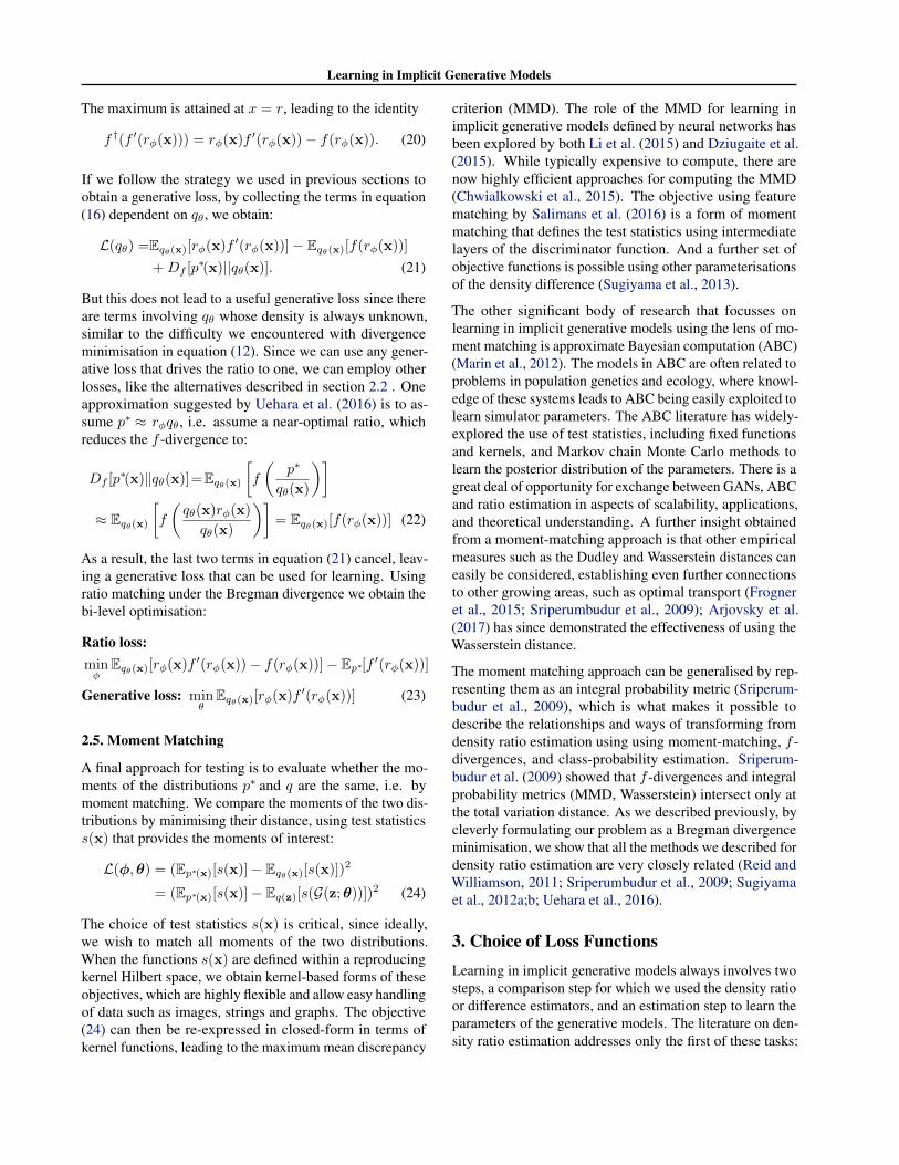
But this does not lead to a useful generative loss since thereare terms involving qθ whose density is always unknown,similar to the difficulty we encountered with divergenceminimisation in equation (12). Since we can use any gener-ative loss that drives the ratio to one, we can employ otherlosses, like the alternatives described in section 2.2 . Oneapproximation suggested by Uehara et al. (2016) is to as-sume p∗ ≈ rφqθ, i.e. assume a near-optimal ratio, whichreduces the f -divergence to:

Df [p∗(x)‖qθ(x)]=Eqθ(x)[f

(p∗

qθ(x)

)]≈ Eqθ(x)

[f

(qθ(x)rφ(x)

qθ(x)

)]= Eqθ(x)[f(rφ(x))] (22)

As a result, the last two terms in equation (21) cancel, leav-ing a generative loss that can be used for learning. Usingratio matching under the Bregman divergence we obtain thebi-level optimisation:

Ratio loss:minφ

Eqθ(x)[rφ(x)f ′(rφ(x))− f(rφ(x))]− Ep∗[f ′(rφ(x))]

Generative loss: minθ

Eqθ(x)[rφ(x)f ′(rφ(x))] (23)

2.5. Moment Matching

A final approach for testing is to evaluate whether the mo-ments of the distributions p∗ and q are the same, i.e. bymoment matching. We compare the moments of the two dis-tributions by minimising their distance, using test statisticss(x) that provides the moments of interest:

L(φ,θ) = (Ep∗(x)[s(x)]− Eqθ(x)[s(x)])2

= (Ep∗(x)[s(x)]− Eq(z)[s(G(z;θ))])2 (24)

The choice of test statistics s(x) is critical, since ideally,we wish to match all moments of the two distributions.When the functions s(x) are defined within a reproducingkernel Hilbert space, we obtain kernel-based forms of theseobjectives, which are highly flexible and allow easy handlingof data such as images, strings and graphs. The objective(24) can then be re-expressed in closed-form in terms ofkernel functions, leading to the maximum mean discrepancy

criterion (MMD). The role of the MMD for learning inimplicit generative models defined by neural networks hasbeen explored by both Li et al. (2015) and Dziugaite et al.(2015). While typically expensive to compute, there arenow highly efficient approaches for computing the MMD(Chwialkowski et al., 2015). The objective using featurematching by Salimans et al. (2016) is a form of momentmatching that defines the test statistics using intermediatelayers of the discriminator function. And a further set ofobjective functions is possible using other parameterisationsof the density difference (Sugiyama et al., 2013).

The other significant body of research that focusses onlearning in implicit generative models using the lens of mo-ment matching is approximate Bayesian computation (ABC)(Marin et al., 2012). The models in ABC are often related toproblems in population genetics and ecology, where knowl-edge of these systems leads to ABC being easily exploited tolearn simulator parameters. The ABC literature has widely-explored the use of test statistics, including fixed functionsand kernels, and Markov chain Monte Carlo methods tolearn the posterior distribution of the parameters. There is agreat deal of opportunity for exchange between GANs, ABCand ratio estimation in aspects of scalability, applications,and theoretical understanding. A further insight obtainedfrom a moment-matching approach is that other empiricalmeasures such as the Dudley and Wasserstein distances caneasily be considered, establishing even further connectionsto other growing areas, such as optimal transport (Frogneret al., 2015; Sriperumbudur et al., 2009); Arjovsky et al.(2017) has since demonstrated the effectiveness of using theWasserstein distance.

The moment matching approach can be generalised by rep-resenting them as an integral probability metric (Sriperum-budur et al., 2009), which is what makes it possible todescribe the relationships and ways of transforming fromdensity ratio estimation using using moment-matching, f -divergences, and class-probability estimation. Sriperum-budur et al. (2009) showed that f -divergences and integralprobability metrics (MMD, Wasserstein) intersect only atthe total variation distance. As we described previously, bycleverly formulating our problem as a Bregman divergenceminimisation, we show that all the methods we described fordensity ratio estimation are very closely related (Reid andWilliamson, 2011; Sriperumbudur et al., 2009; Sugiyamaet al., 2012a;b; Uehara et al., 2016).

3. Choice of Loss FunctionsLearning in implicit generative models always involves twosteps, a comparison step for which we used the density ratioor difference estimators, and an estimation step to learn theparameters of the generative models. The literature on den-sity ratio estimation addresses only the first of these tasks:

Learning in Implicit Generative Models

where only the density ratio is to be estimated, Sugiyamaet al. (2012a) provide guidance on this choice. But when welearn implicit generative models, we have two loss functions,and these loss functions need not be coupled to each other.Poole et al. (2016) independently proposed using differentf divergences for ratio loss and the generator loss.

Evaluation. While natural to ask which loss functionshould be used, this choice is not clear due to the challengesin evaluating implicit models. In prescribed models, thestandard approach for evaluation involves computation ofthe marginalised likelihood, but is not generally possible inimplicit models. Estimates of the likelihood can be obtainedusing kernel density estimators, but this is highly-unreliable,especially in high-dimensions (Theis et al., 2015). Most pa-pers rely on visual inspection that can be misleading, sincemode-collapse (where the generated samples sample fromonly a few modes) and memorisation of the training datacannot be detected easily. Other approaches for evaluationinclude reporting the value of the density ratio, a quantitywe can always compute using the approaches described, theuse of annealed importance sampling Wu et al. (2016), useof empirical distance metric such as the MMD (Sutherlandet al., 2016) or the Wasserstein distance (Arjovsky et al.,2017). But we still lack the tools to make theoretical state-ments that allow us to assess the correctness of the modellearning framework, although theoretical developments inthe literature on approximate Bayesian computation mayhelp in this regard, e.g., Frazier et al. (2016).

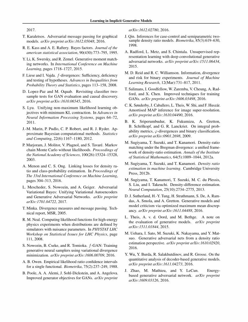
Training considerations. As discussed, density ratiomatching gives us guidance only on the choice of ratioloss. In implicit models, we not only require a good ap-proximation for the density ratio, but also need to ensurethat we are able to train the generator efficiently. A mean-ingful f divergence requires the support of the distribu-tions to overlap and it is common to add instance noise(Arjovsky and Bottou, 2017; Sønderby et al., 2016) to en-sure this. Additionally, when using gradient based meth-ods, we need to ensure that the generator gradients do notvanish. For simplicity, consider the scenario where the im-plicit model is learnt using the (approximate) f -divergenceEx∼qθ(x)f(r∗(x)) ≈ Ex∼qθ(x)f(rφ(x)) using gradient de-scent. We visualise f(r) for several choices of f in Figure 2.During the initial phase of training, r is very close to 0 forsamples generated from q. When optimising the model pa-rameters θ, we require that the gradient f ′(r) be non-zerofor r � 0. We observe that the f corresponding to KL,chi-squared and minimax is fairly flat when log r < 0 andhence difficult to train. For this reason, Goodfellow et al.(2014) use an alternative loss when training the generator,but which has the same fixed points. We observe that fcorresponding to the alternative loss as well as the reverseKL provide stronger gradients when log r < 0. Similar phe-nomena are observed when optimising the model according

−5 −4 −3 −2 −1 0 1 2log r

−2

0

2

4

6

8

10

f(r)

minimax: ¡log(1+ r)ALT: ¡log(1+1=r)Reverse KL: ¡log rKL (ML): r log r

Chi-squared: (r¡ 1)2

Figure 2. Objective functions for different choices of f .

to (10) and (23). Hence, f -GANs (Nowozin et al., 2016)and b-GANs (Uehara et al., 2016) optimise alternative losses(with same fixed points) which provide stronger gradients.Moment matching methods do not suffer from the aforemen-tioned vanishing-gradient issue. However, they are compu-tationally more expensive than training a classifier, and mayrequire larger batch sizes to ensure that the moments are ap-proximated accurately. Wasserstein GANs (Arjovsky et al.,2017) are promising as they solve the vanishing-gradientissue in a computationally efficient manner.

4. DiscussionBy using an inferential principle driven by hypothesis test-ing, we have been able to develop a number of indirectmethods for learning the parameters of generative models.These methods do not compute the probability of the dataor posterior distributions over latent variables, but insteadonly involve relative statements of probability by compar-ing populations of data from the generative model to ob-served data. This view allows us to better understand howalgorithms such as generative adversarial networks, approx-imate Bayesian computation, noise-contrastive estimation,and density ratio estimation are related. Ultimately, thesetechniques make it possible for us to make contributions toapplications in climate and weather, economics, populationgenetics, and epidemiology, all areas whose principal toolsare implicit generative models.

Distinction between implicit and prescribed models.The distinction between implicit and prescribed models isuseful to keep in mind for at least two reasons: the choice ofmodel has direct implications on the types of learning andinferential principles that can be called upon; and it makesexplicit that there are many different ways in which to spec-ify a model that captures our beliefs about data generatingprocesses. Any implicit model can be easily turned into aprescribed model by adding a simple likelihood function(noise model) on the generated outputs, so the distinctionis not essential. And models with likelihood functions alsoregularly face the problem of intractable marginal likeli-

Learning in Implicit Generative Models

hoods. But the specification of a likelihood function pro-vides knowledge of p∗ that leads to different algorithms byexploiting this knowledge, e.g., NCE resulting from class-probability based testing in un-normalised models (Gut-mann and Hyvärinen, 2012), or variational lower boundsfor directed graphical models. We strive to maintain a cleardistinction between the choice of model, choice of infer-ence, and the resulting algorithm, since it is through such astructured view that we can best recognise the connectionsbetween research areas that rely on the same sets of tools.

Model misspecification and non-maximum likelihoodmethods. Once we have made the choice of an implicit gen-erative model, we cannot use likelihood-based techniques,which then makes testing and estimation-by-comparisonappealing. What is striking, is that this leads us to principlesfor parameter learning that do not require inference of anyunderlying latent variables, side-stepping one of the majorchallenges in statistical practice. This piques our interest inmore general approaches for non-maximum likelihood andlikelihood-free estimation methods, of which there is muchwork (Frogner et al., 2015; Gutmann and Hyvärinen, 2012;Hall, 2005; Lyu, 2011; Marin et al., 2012). We often dealwith misspecified models where qθ cannot represent p∗, andnon maximum likelihood methods could be a more robustchoice depending on the task (see figure 1 in (Huszár, 2015)for an illustrative example).

Bayesian inference and message passing. We have mainlydiscussed point estimation methods for parameter learning.It is also desirable to perform Bayesian inference in im-plicit models, where we learn the posterior distribution overthe model parameters p(θ|x), allowing knowledge of pa-rameter uncertainty to be used in risk minimisation andother decision-making tasks. This is the aim of approximateBayesian computation (ABC) (Marin et al., 2012). Themost common approach for thinking about ABC is throughmoment-matching, but as we explored, there are other ap-proaches available. An approach through class-probabilityestimation is appealing and leads to classifier ABC (Gut-mann et al., 2014). We have highly diverse approaches forBayesian reasoning in prescribed models, and it is desirableto develop a similar breadth of choice for implicit models.

Implicit models allow for a natural approach for amortisedinference, and can be used whenever we wish to to learndistributions from which we do not wish to evaluate proba-bilities but only generate samples. Consequently, whereverwe see density-ratios or density-differences in probabilisticmodelling, we can make use of implicit models and bi-leveloptimisation, such as in importance sampling, variational in-ference, or message passing. For example, Karaletsos (2016)use GAN-like techniques for inference in factor graphs, andsince the central quantity of variational inference is a den-sity ratio it is possible to propose a modified variational

inference using implicit models, as discussed by Meschederet al. (2017) and Huszár (2017).

Perceptual losses. Several authors have also proposed us-ing pre-trained discriminative networks to define the testfunctions since the difference in activations (of say a pre-trained VGG classifier) can better capture perceptual sim-ilarity than the reconstruction error in pixel space. Thisprovides a strong motivation for further research into jointmodels of images and labels. However, it is not completelyunsupervised as the pre-trained discriminative network con-tains information about labels and invariances. This makesevaluation difficult since we lack good metrics and can onlyfairly compare to other joint models that use both label andimage information.

Non-differentiable models. We have restricted our devel-opment to implicit models that are differentiable. In manypractical applications, the implicit model (or simulator) willbe non-differentiable, discrete or defined in other ways, suchas through a stochastic differential equation . The stochas-tic optimisation problem we are generally faced with (fordifferentiable and non-differentiable models), is to compute∆ = ∇θEqθ(x)[f(x)], the gradient of the expectation ofa function. As our exposition followed, when the implicitmodel is differentiable, the pathwise derivative estimator canbe used, i.e. ∆ = Eq(z)[∇θf(Gθ(z))] by rewriting the ex-pectation in terms of the known and easy to sample distribu-tion q(z). It is commonly assumed that when we encounternon-differentiable functions that the score function estimator(or likelihood ratio or reinforce estimator) can be used; thescore-function estimator is ∆ = Eqθ(x)[f(x)∇θ log qθ(x)].For implicit models, we do not have knowledge of the den-sity q(x) whose log derivative we require, making this es-timator inapplicable. This leads to the first of three toolsavailable for non-differentiable models: weak derivative andrelated stochastic finite difference estimators, which requireforward-simulation only and compute gradients by pertur-bation of the parameters (Fu, 2005; Glasserman, 2003).

The two other approaches are: moment matching and ABC-MCMC (Marjoram et al., 2003), which has been successfulfor many problems with moderate dimension; and the nat-ural choice of gradient-free optimisation methods, whichinclude familiar tools such as Bayesian optimisation (Gut-mann and Corander, 2016), evolutionary search like CMA-ES, and the Nelder-Mead method, amongst others (Connet al., 2009). For all three approaches, new insights will beneeded to help scale to high-dimensional data with complexdependency structures.

Ultimately, these concerns serve to highlight the many op-portunities that remain for advancing our understandingof inference and parameter learning in implicit generativemodels.

Learning in Implicit Generative Models

ACKNOWLEDGEMENTS

We thank David Pfau, Lars Buesing, Guillaume Desjardins,Theophane Weber, Danilo Rezende, Charles Blundell, IrinaHiggins, Yee Whye Teh, Avraham Ruderman, BrendanO’Donoghue and Ivo Danihelka for helpful feedback anddiscussions. We thank Cheng Soon Ong for an insightfulconversation that helped to make an initial connection.

ReferencesS. M. Ali and S. D. Silvey. A general class of coefficients of

divergence of one distribution from another. Journal ofthe Royal Statistical Society. Series B (Methodological),pages 131–142, 1966.

M. Arjovsky and L. Bottou. Towards principled methods fortraining generative adversarial networks. In NIPS 2016Workshop on Adversarial Training. In review for ICLR,2017.

M. Arjovsky, S. Chintala, and L. Bottou. Wasserstein GAN.arXiv preprint arXiv:1701.07875, 2017.

S. Bickel, J. Bogojeska, T. Lengauer, and T. Scheffer. Multi-task learning for HIV therapy screening. In Proceedingsof the 25th international conference on Machine learning,pages 56–63. ACM, 2008.

A. Buja, W. Stuetzle, and Y. Shen. Loss functions for binaryclass probability estimation and classification: Structureand applications. Working draft, November, 2005.

K. P. Chwialkowski, A. Ramdas, D. Sejdinovic, and A. Gret-ton. Fast two-sample testing with analytic representationsof probability measures. In Advances in Neural Informa-tion Processing Systems, pages 1981–1989, 2015.

B. Colson, P. Marcotte, and G. Savard. An overview ofbilevel optimization. Annals of operations research, 153(1):235–256, 2007.

A. R. Conn, K. Scheinberg, and L. N. Vicente. Introductionto derivative-free optimization, volume 8. Siam, 2009.

K. Cranmer, J. Pavez, and G. Louppe. Approximating like-lihood ratios with calibrated discriminative classifiers.arXiv preprint arXiv:1506.02169, 2015.

A. Creswell and A. A. Bharath. Task specific adversarialcost function. arXiv preprint arXiv:1609.08661, 2016.

I. Csiszàr. Information-type measures of difference of prob-ability distributions and indirect observations. Studia Sci-entiarum Mathematicarum Hungarica, 2:299–318, 1967.

L. Devroye. Non-uniform random variate generation. Hand-books in operations research and management science,13:83–121, 2006.

P. J. Diggle and R. J. Gratton. Monte Carlo methods of infer-ence for implicit statistical models. Journal of the RoyalStatistical Society. Series B (Methodological), pages 193–

227, 1984.

G. K. Dziugaite, D. M. Roy, and Z. Ghahramani. Traininggenerative neural networks via maximum mean discrep-ancy optimization. arXiv preprint arXiv:1505.03906,2015.

D. T. Frazier, G. M. Martin, C. P. Robert, and J. Rousseau.Asymptotic properties of approximate Bayesian compu-tation. arXiv preprint arXiv:1607.06903, 2016.

C. Frogner, C. Zhang, H. Mobahi, M. Araya, and T. A.Poggio. Learning with a Wasserstein loss. In Advancesin Neural Information Processing Systems, pages 2053–2061, 2015.

M. C. Fu. Stochastic gradient estimation. Technical report,DTIC Document, 2005.

K. Fukunaga and L. Hostetler. The estimation of the gra-dient of a density function, with applications in patternrecognition. IEEE Transactions on information theory,21(1):32–40, 1975.

P. Glasserman. Monte Carlo methods in financial engineer-ing, volume 53. Springer Science & Business Media,2003.

T. Gneiting and A. E. Raftery. Strictly proper scoring rules,prediction, and estimation. Journal of the American Sta-tistical Association, 102(477):359–378, 2007.

I. Goodfellow, J. Pouget-Abadie, M. Mirza, B. Xu,D. Warde-Farley, S. Ozair, A. Courville, and Y. Ben-gio. Generative adversarial nets. In Advances in NeuralInformation Processing Systems, pages 2672–2680, 2014.

M. U. Gutmann and J. Corander. Bayesian optimizationfor likelihood-free inference of simulator-based statisticalmodels. Journal of Machine Learning Research, 17(125):1–47, 2016.

M. U. Gutmann and A. Hyvärinen. Noise-contrastive estima-tion of unnormalized statistical models, with applicationsto natural image statistics. Journal of Machine LearningResearch, 13(Feb):307–361, 2012.

M. U. Gutmann, R. Dutta, S. Kaski, and J. Corander. Statis-tical inference of intractable generative models via classi-fication. arXiv preprint arXiv:1407.4981, 2014.

A. R. Hall. Generalized method of moments. Oxford Uni-versity Press, 2005.

T. Hastie, R. Tibshirani, and J. Friedman. The elements ofstatistical learning. Springer, pp 495–497, 10th printing,2nd edition, 2013.

F. Huszár. How (not) to train your generative model: Sched-uled sampling, likelihood, adversary? arXiv preprintarXiv:1511.05101, 2015.

F. Huszár. Variational inference using implicit models, partI: Bayesian logistic regression. https://goo.gl/oDFqJH,

Learning in Implicit Generative Models

2017.

T. Karaletsos. Adversarial message passing for graphicalmodels. arXiv preprint arXiv:1612.05048, 2016.

R. E. Kass and A. E. Raftery. Bayes factors. Journal of theamerican statistical association, 90(430):773–795, 1995.

Y. Li, K. Swersky, and R. Zemel. Generative moment match-ing networks. In International Conference on MachineLearning, pages 1718–1727, 2015.

F. Liese and I. Vajda. f -divergences: Sufficiency, deficiencyand testing of hypotheses. Advances in Inequalities fromProbability Theory and Statistics, pages 113–158, 2008.

D. Lopez-Paz and M. Oquab. Revisiting classifier two-sample tests for GAN evaluation and causal discovery.arXiv preprint arXiv:1610.06545, 2016.

S. Lyu. Unifying non-maximum likelihood learning ob-jectives with minimum KL contraction. In Advances inNeural Information Processing Systems, pages 64–72,2011.

J.-M. Marin, P. Pudlo, C. P. Robert, and R. J. Ryder. Ap-proximate Bayesian computational methods. Statisticsand Computing, 22(6):1167–1180, 2012.

P. Marjoram, J. Molitor, V. Plagnol, and S. Tavaré. Markovchain Monte Carlo without likelihoods. Proceedings ofthe National Academy of Sciences, 100(26):15324–15328,2003.

A. Menon and C. S. Ong. Linking losses for density ra-tio and class-probability estimation. In Proceedings ofThe 33rd International Conference on Machine Learning,pages 304–313, 2016.

L. Mescheder, S. Nowozin, and A. Geiger. AdversarialVariational Bayes: Unifying Variational Autoencodersand Generative Adversarial Networks. arXiv preprintarXiv:1701.04722, 2017.

T. Minka. Divergence measures and message passing. Tech-nical report, MSR, 2005.

R. M. Neal. Computing likelihood functions for high-energyphysics experiments when distributions are defined bysimulators with nuisance parameters. In PHYSTAT LHCWorkshop on Statistical Issues for LHC Physics, page111, 2008.

S. Nowozin, B. Cseke, and R. Tomioka. f -GAN: Traininggenerative neural samplers using variational divergenceminimization. arXiv preprint arXiv:1606.00709, 2016.

A. B. Owen. Empirical likelihood ratio confidence intervalsfor a single functional. Biometrika, 75(2):237–249, 1988.

B. Poole, A. A. Alemi, J. Sohl-Dickstein, and A. Angelova.Improved generator objectives for GANs. arXiv preprint

arXiv:1612.02780, 2016.

J. Qin. Inferences for case-control and semiparametric two-sample density ratio models. Biometrika, 85(3):619–630,1998.

A. Radford, L. Metz, and S. Chintala. Unsupervised rep-resentation learning with deep convolutional generativeadversarial networks. arXiv preprint arXiv:1511.06434,2015.

M. D. Reid and R. C. Williamson. Information, divergenceand risk for binary experiments. Journal of MachineLearning Research, 12(Mar):731–817, 2011.

T. Salimans, I. Goodfellow, W. Zaremba, V. Cheung, A. Rad-ford, and X. Chen. Improved techniques for trainingGANs. arXiv preprint arXiv:1606.03498, 2016.

C. K. Sønderby, J. Caballero, L. Theis, W. Shi, and F. Huszár.Amortised MAP inference for image super-resolution.arXiv preprint arXiv:1610.04490, 2016.

B. K. Sriperumbudur, K. Fukumizu, A. Gretton,B. Schölkopf, and G. R. Lanckriet. On integral prob-ability metrics, ϕ-divergences and binary classification.arXiv preprint arXiv:0901.2698, 2009.

M. Sugiyama, T. Suzuki, and T. Kanamori. Density-ratiomatching under the Bregman divergence: a unified frame-work of density-ratio estimation. Annals of the Instituteof Statistical Mathematics, 64(5):1009–1044, 2012a.

M. Sugiyama, T. Suzuki, and T. Kanamori. Density ratioestimation in machine learning. Cambridge UniversityPress, 2012b.

M. Sugiyama, T. Kanamori, T. Suzuki, M. C. du Plessis,S. Liu, and I. Takeuchi. Density-difference estimation.Neural Computation, 25(10):2734–2775, 2013.

D. J. Sutherland, H.-Y. Tung, H. Strathmann, S. De, A. Ram-das, A. Smola, and A. Gretton. Generative models andmodel criticism via optimized maximum mean discrep-ancy. arXiv preprint arXiv:1611.04488, 2016.

L. Theis, A. v. d. Oord, and M. Bethge. A note onthe evaluation of generative models. arXiv preprintarXiv:1511.01844, 2015.

M. Uehara, I. Sato, M. Suzuki, K. Nakayama, and Y. Mat-suo. Generative adversarial nets from a density ratioestimation perspective. arXiv preprint arXiv:1610.02920,2016.

Y. Wu, Y. Burda, R. Salakhutdinov, and R. Grosse. On thequantitative analysis of decoder-based generative models.arXiv preprint arXiv:1611.04273, 2016.

J. Zhao, M. Mathieu, and Y. LeCun. Energy-based generative adversarial network. arXiv preprintarXiv:1609.03126, 2016.