Learning, Forecasting and Structural Breaks1

Learning, Forecasting and Structural Breaks1

July 2004

John M. MaheuDepartment of Economics

University of TorontoToronto, Ontario

M5S 3G7Canada

[email protected]

Stephen GordonDepartement d’economique and CIRPEE

Universite LavalQuebec City, Quebec

G1K 7P4Canada

[email protected]

AbstractThe literature on structural breaks focuses on ex post identification of break points that mayhave occurred in the past. While this question is important, a more challenging problemfacing econometricians is to provide forecasts when the data generating process is unstable.The purpose of this paper is to provide a general methodology for forecasting in the presenceof model instability. We make no assumptions on the number of break points or the law ofmotion governing parameter changes. Our approach makes use of Bayesian methods of modelcomparison and learning in order to provide an optimal predictive density from which forecastscan be derived. Estimates for the posterior probability that a break occurred at a particularpoint in the sample are generated as a byproduct of our procedure. We discuss the importanceof using priors that accurately reflect the econometrician’s opinions as to what constitutes aplausible forecast. Several applications to macroeconomic time-series data demonstrate theusefulness of our procedure.

Keywords: Bayesian Model Averaging, Markov Chain Monte Carlo, Real GDP Growth, Phillip’sCurve

1Both authors are grateful for financial support from the Social Sciences and Humanities ResearchCouncil of Canada.

1 Introduction

There is a considerable body of evidence that documents the instability of many im-portant relationships among economic variables. Popular examples include the Phillip’scurve, U.S. interest rates and the demand for money.2 An important challenge facingmodern economics is the modeling of these unstable relationships. For econometricians,the difficulties involve estimation, inference and forecasting in the presence of possiblestructural instability.

Classical approaches to the identification of break points are based on asymptotictheory - see, for example, Ghysels and Hall (1990), Hansen (1992), Andrews (1993),Dufour, Ghysels, and Hall (1994), Ghysels, Guay, and Hall (1997), and Andrews (2003)- are based on frameworks in which both the pre-break and post-break data samples goto infinity.3 Moreover, tests for multiple breaks such as those proposed by Andrews, Lee,and Ploberger (1996), and Bai and Perron (1998) are also based on similar hypotheses.In applications that make use of available finite data sets, the empirical relevance of suchan assumption may be suspect. Furthermore, the statistical properties of a forecastingmodel based on classical breakpoint tests are far from clear, since such a model wouldbe based on a pre-test estimator.

In contrast, Bayesian approaches to the problem are theoretically simple, are basedon finite-sample inference, and typically take the form of a simple model comparisonexercise. Examples include Inclan (1994), Chib (1998), Wang and Zivot (2000), Kim,Nelson, and Piger (2004) and Pasaran, Pettenuzzo, and Timmermann (2004) whichemploy Markov Chain Monte Carlo sampling methods to make posterior inferences re-garding the timing of break points in a given sample.

A feature that is common to both strands of the existing literature is the focus on theex post identification of structural breaks that may have occurred in the past. While thisquestion is of course important in itself, economists are more likely to be interested inmaking forecasts when the the data generating process is unstable. This is the questionthat we address here. More precisely, we focus on the question of how to make optimaluse of past data to forecast out-of-sample while taking into account the possibility thatbreaks have occurred in the past, as well as the possibility that they may occur in thefuture.

We present a general methodology for economic decision making based on a modelsubject to structural breaks. Our analysis uses adaptive learning via Bayes’ rule in orderto make optimal use of past data to make forecasts. No assumptions concerning breaktimes or their impact on model parameters are made.4 As a byproduct, our procedure

2Stock and Watson (1996) suggest that the laws of motion governing the evolution of many importantmacroeconomic time series appear to be unstable.

3The theory of Dufour, Ghysels, and Hall (1994) and Andrews (2003) only requires that the struc-turally stable portion of the data goes to infinity.

4Pasaran, Pettenuzzo and Timmermann focus on forecasting in the presence of breaks. Extendingthe work of Chib (1998) and Carlin, Gelfand, and Smith (1992), breaks are assumed to be governed bya first-order Markov chain, while break parameters are drawn from a common distribution. Nonlinear

1

also provides estimates for the posterior probability that a break point occurred any-where in the sample, as well as the posterior distribution for the number of observationsthat would be useful in making out-of-sample forecasts at any point in the sample.

The approach of this paper is most easily seen with a simple example. Consider theobservations yj, j = 1, ..., t and suppose that an analyst wishes to forecast the value ofyt+1. Let M denote the hypothesis that yt+1 will be drawn from the same process thatgenerated the previous observations. Conditional on M being true, then It ≡ {y1, . . . , yt}can be used to to construct a predictive data density, denoted by p(yt+1|It,M). Supposenow that the analyst wishes to take into account the possibility that M may not becorrect, and that yt+1 will be drawn from an entirely different distribution; denoted byM∗, the hypothesis that a structural break will occur between t and t + 1. If M∗ iscorrect, the past data contained in It will be useless in predicting yt+1, so the analystwill be obliged to specify a predictive density of the form p(yt+1|M∗) using his subjectivejudgment.

Suppose that the analyst attaches a subjective probability λt+1 that M∗ is true.Then the predictive density of yt+1 is the following mixture:

p(yt+1|It) = p(yt+1|It,M)[1− λt+1] + p(yt+1|M∗)λt+1,

from which any quantity of interest, such as predictive moments or quantiles, can becalculated.5 The first term on the right hand side is the predictive density conditional onno structural break (using all available data) weighted by the probability of no structuralbreak. The second term is the predictive density conditional on a structural break basedon the subjective beliefs of the analyst, weighted by the probability of a structural break.

After observing yt+1, the information set is updated so that It+1 = {It, yt+1}. Theprobability that there was a structural break between t and t + 1 can be updated ac-cording to Bayes’ rule:

p(M∗|It+1) =λt+1p(yt+1|It,M∗)

[1− λt+1]p(yt+1|It,M) + λt+1p(yt+1|It,M∗)

and p(M |It+1) = 1−p(M∗|It+1). Conditional on M and M∗, the predictive distributionsfor yt+2 can be updated to include the information contained in yt+1. If we denote byM the hypothesis that there is no structural break between t+ 1 and t+ 2, we note that

p(yt+2|It+1, M) = p(yt+2|It+1,M)p(M |It+1) + p(yt+2|It+1,M∗)p(M∗|It+1).

models such as regime switching models (Hamilton (1989)), and time-varying parameter models (Kimand Nelson (1999), Koop and Potter (2001), McCulloch and Tsay (1993) , Nicholls and Pagan (1985))allow for changes in the form of the conditional density of the data, but these are assumed to evolveaccording to a fixed law of motion. Parameters change over time, but in a predictable way.

5From a Bayesian perspective all inferential information regarding future outcomes of yt+1, condi-tional on It and a model, is contained in the predictive density.

2

Suppose now that the econometrician wishes to take into account the hypothesis,denoted by M∗, that there may be a structural break between t + 1 and t + 2. In thiscase, he would specify a predictive distribution of the form p(yt+2|M∗) and a subjectiveprobability 0 ≤ λt+2 ≤ 1 that M∗ is correct, and the above exercise would be repeated.6

At each data point, a new model is introduced and standard results from Bayesianmodel averaging provide predictive quantities as well as model probabilities. Since amodel is defined by the time period it starts, their probabilities can be used to identifybreaks in the past. As the empirical examples illustrate, our method provides a richset of information with regard to model probabilities, posterior parameter densities,and forecasts, all as a function of time. By construction, forecasts incorporate bothparameter uncertainty and model uncertainty.

Several applications of the theory to simulated, and macroeconomic time-series dataare discussed. In comparison to a model that assumes no breaks, we find the methodproduces very good out-of-sample forecasts, accurately identifies breaks, and performswell when the data do not contain breaks. In particular, the examples demonstrate thata break can result in a large jump in the predictive variance, which quickly reduces aswe learn about the new parameters. However, models that ignore breaks, may have along-term rise in the predictive variance. As a result, our method can be expected toproduce more realistic moments, and quantiles of the predictive density.

We consider predictions of real U.S. GDP and document the reduction in variabilitydiscussed in Stock and Watson (2002) among others. Rather than a one time break involatility, our results point to a gradual reduction in volatility over time with evidenceof 3 separate regimes. The model is particularly useful in forecasting the probability ofexpansions. A second application considers a forecasting model of inflation motivatedfrom a Phillips curve relationship. There are several breaks in this model and a consid-erable amount of parameter instability. By accounting for these breaks in the process,our approach delivers improved forecasting precision for inflation. The identified breaks,which are not exclusively associated with oil shocks, indicate that the Phillips curvewe use is far from stable. However, the structural break model optimally extracts anypredictive value from this unstable relationship.

This paper is organized as follows. Section 2 provides a more detailed explanation ofthe approach, as well as a description of techniques that can be used to implement theprocedure. Section 3 applies these methods to simulated data, growth rates in US GDPand to a Phillips curve model of inflation. Section 4 discusses results and extensions.

2 Learning about structural breaks

In this section we provide details of the structural break model and how to forecast inthe presence of breaks as well as various posterior quantities that are useful in assessingthe impact of structural breaks on a model. In the following we consider a univariate

6In the empirical applications we repeat this exercise for all observations in the sample.

3

time-series context, however, the calculations generalize to multivariate models withweakly exogenous regressors in the obvious way. As in the Introduction, let yt be anobservation, and It = {y1, ..., yt}, the information set available at time t.

The first step in making the approach operational is to introduce the role of param-eters in learning and forecasting in the presence of structural breaks. Let p(yt|θ, It−1)denote the predictive density from a model, conditional on past data It−1, and condi-tional on a parameter vector θ. For simplicity, we assume that the form of this densityis constant throughout the exercise, and that structural breaks are characterized by un-predictable changes in the value of θ. Extensions to the case where the conditional datadensity changes over time are straightforward, as noted in Section 2.1 below.

Let Mi be a model in which it is supposed that a structural break occurred betweenperiods i − 1 and i7, while p(θ|Mi) is the prior distribution for θ conditional on thehypothesis that model Mi is correct. In the case of model Mi, data before the break,y1, ..., yi−1 is not useful in parameter estimation, so the posterior p(θ|It−1,Mi) is obtainedaccording to

p(θ|It−1,Mi) =p(yi, ..., yt−1|θ,Mi)p(θ|Mi)∫p(yi, ..., yt−1|θ,Mi)p(θ|Mi) dθ

, i < t (1)

p(θ|It−1,Mi) =p(θ|Mi), i = t. (2)

Given the conditional data density p(yt|θ, It−1,Mi) and the posterior p(θ|It−1,Mi),the predictive density is

p(yt|It−1,Mi) =

∫p(yt|θ, It−1,Mi)p(θ|It−1,Mi) dθ. (3)

Since no structure has been put on the form or the rate of arrival of structural breaks,the econometrician is obliged to make a subjective assessment about the probabilitythat a break will occur between t − 1 and t. This subjective probability is denotedby 0 ≤ λt ≤ 1; λt may vary as the econometrician’s assessment of the rate of arrivalof breaks evolves over time. If λj > 0, j = 1, .., t − 1 there will be a total of t − 1models available at time t− 1, and whose relative weights will have updated over timeaccording to Bayes’ rule. The predictive density for yt is obtained by integrating acrossthe available models:

p(yt|It−1) =

[t−1∑i=1

p(yt|It−1,Mi)p(Mi|It−1)

](1− λt) + λtp(yt|It−1,Mt). (4)

The final term on the right-hand side of (4) is the probability of a break multiplied bythe predictive density conditional on a break occurring between t− 1 and t. Therefore,p(yt|It−1,Mt) is based only on the prior p(θ|Mt), and not a function of past data. How-ever, future data {yt+1, yt+2, ...}, is used to learn about the new value of θ. If λt = 0,then model Mt receives no weight.

7In other words yi−1 and yi are drawn from different data generating processes.

4

After observing yt, model probabilities can be updated through Bayes’ rule. Forinstance,

p(Mi|It) =(1− λt)p(yt|It−1,Mi)p(Mi|It−1)

p(yt|It−1), 1 ≤ i < t (5)

p(Mt|It) =λtp(yt|It−1,Mt)

p(yt|It−1)i = t. (6)

At time t there are a maximum of t models that are being entertained. Any featureof the posterior distribution of θ can be calculated by Bayesian model averaging. Forexample, if h(θ) is a function of the parameter vector then its expected value is

E[h(θ)|It] =t∑i=1

E[h(θ)|It,Mi]p(Mi|It). (7)

Similarly, there are t+1 models that contribute to the predictive density, and if g(yt+h), h ≥1, is a function of yt+h then8

E[g(yt+h)|It] =t∑i=1

E[g(yt+h)|It,Mi]p(Mi|It)(1− λt+1) + E[g(yt+h)|It,Mt+1]λt+1. (8)

Note that with the appropriate definition of h(·) and g(·), we can recover any momentof interest or probability. Quantiles can be calculated through simulation. In this case,a draw from the models, based on the model probabilities is first taken before a modelspecific feature is sampled such as a parameter or the simulation of a future observation.Collecting a large number of draws and ordering them allows for the estimation of aquantile.

Since models are identified with particular start-up points, they represent breakpoints. That is, models with high posterior probability identify structural breaks points.For example, if model Mi has a large model probability among all candidate models, itsuggests that a break occurred at time i. A plot of the maximum model probability asa function of time may be informative as to when breaks occurs and how confident weare in the new model. Similarly, a time series plot of E[θ|It] presents evidence regardingstructural change of the parameter θ through time.

Another useful posterior summary measure of structural breaks is mean useful ob-servations (MUO). For instance, if there were 100 data points and it was known that abreak occurred in the past at observation 45 then only 55 observations would be usefulin estimating the post break model. Mean useful observations is a plot of the expectednumber of useful observations at a point in time and is calculated at time t as,

MUOt =t∑i=1

(t− i+ 1)p(Mi|It). (9)

8Note that we have implicitly assumed one break occurs over the forecast horizon, however, it ispossible that multiple breaks occur at t+1, t+2, ..., t+h. This can be accounted for, as in Equation (8),by integrating over all possible break permutations.

5

In the circumstance where no breaks occur, MUOt as a function of time would be a 45degree line. However, when a break occurs MUOt drops below the 45 degree line.

2.1 Prior specification

A coherent model of learning requires that the predictive density for each model Mi mustbe a proper density. In the current context, where the predictive density p(yt+1|It,Mi)defined by the mixture in (3) above, this condition will be satisfied if p(θ|It,Mi) is aproper density. If at time t, the number of observations since the breakpoint associatedwith model i, that is the difference t−i is sufficiently large, then p(θ|It,Mi) will generallybe proper even if the original prior p(θ|Mi) is an improper ’ignorance prior’.

The use of improper priors or even highly diffuse priors is clearly inappropriate here.It may take many observations before p(θ|It,Mi) is concentrated enough to generatepredictive distributions that would receive any significant support. For an econometri-cian who is trying to generate forecasts using available data, there are significant gainsin being able to respond more quickly to the possibility that a break may have occurredrecently. Our approach is to adopt proper priors that produce reasonable predictivedistributions. Simulating a model based on the prior, and considering the empiricalmoments is often helpful in selecting prior parameters.

We find it convenient to use the same form for p(θ|Mi) at each data point in theempirical applications below, but this restriction can be relaxed. For example, if theparameter vector θ can be decomposed according to θ = (θ0, θ1), and if the analystbelieves that any potential instability can be attributed to changes in θ0 - that is, theanalyst believes that θ1 is stable - then an appropriate prior might be one where themarginal prior p(θ1|Mi) resembles the marginal posterior p(θ1|Ii).

Similarly, there is no obvious reason why an analyst should insist on using the samevalue for the λt in every period. If, in his subjective judgment, his model has beenproducing satisfactory forecasts, and if nothing has occurred that would suggest a recentbreak, he may choose an extremely low value of λt. On the other hand, if he sees a markeddecline in the quality of his forecasts, then he might think it appropriate to set λt at alarger value. In our inflation example below, we find that an ad hoc rule in which λt ismodeled as an increasing function on the size of past forecast errors does quite well.

The approach discussed in the previous section can also be adapted to the case wherethe structural instability of the data-generating process is manifested by changes in theform of the conditional data density itself, as noted above. The simplest way wouldbe to simply introduce more than one data density in each period. Suppose that theanalyst believes that if there is a break after period t, there are K possibilities for thedata density in period t+ 1, denoted by pk(yt+1|θk,Mk

t+1), each accompanied by a priorp(θk|Mk

t+1). Suppose also that the analyst assigns the probability λkt+1 to Mkt+1. In this

context, the hypothesis Mt+1, that there was a break immediately following period t,is defined by Mt+1 ≡ {Mk

t+1}Kk=1, and its prior probability is λt+1 =∑K

k=1 λkt+1. The

6

predictive distribution conditional on a break, is the mixture

p(yt+1|Mt+1) =K∑

k=1

[∫p(yt+1|θk,Mk

t+1)p(θk|Mkt+1) dθk

](λkt+1/λt+1).

After yt+1 is observed, the model probabilities p(Mkt+1|It+1) and distributions p(θk|Mk

t+1, It+1)are updated in the usual way. Note also that there is no reason to restrict attention tothe case where the number of potential models is fixed over time.

2.2 Computational Issues

For many econometric models, all of the quantities discussed in the previous subsectioncan be calculated using standard Bayesian simulation methods. For an introduction toMarkov chain Monte Carlo (MCMC) see Koop (2003) while Chib (2001), Geweke (1998)Robert and Casella (1999) provide a detailed survey of MCMC methods.

The following steps are required for model estimation at time t:

1. Obtain a sample from the posterior of model Mi, i = 1, ..., t+1. Calculate posteriorquantities for each of the t models or predictive features of interest for the t + 1models. Note that Mt+1 is the prior and an input onto forecasting.

2. Calculate model probabilities, p(Mi|It), i = 1, ..., t.

3. Perform model averaging on quantities of interest, forecasts, etc., using equations(7) and (8). λt coupled with the model probabilities from step 2 give the t + 1model probabilities used in forecasting.

Typically, and in our applications, we repeat the above steps for all observation t =1, ..., T . However, various schemes in which breaks are permitted at periodic timescould be considered by setting the appropriate subset of {λt}Tt=1 to 0.

In the special case of the linear model with a conjugate normal-gamma prior ananalytical solution is available for the posterior in Step 1. In other cases, Gibbs orMetropolis-Hasting sampling can be used to obtain a sample from the posterior. Thereare several approaches that can be used to calculate the marginal likelihood and thereforethe model probabilities. These include Chib (1995), Gelfand and Dey (1994), Geweke(1995), and Newton and Raftery (1994).

3 Empirical Examples

In this section we present results from simulated data and two examples in macroeco-nomics. In both cases we consider the following linear model,

yt = Xt−1β + εt, εt ∼ N(0, σ2) (10)

7

where yt is the variable of interest that is assumed to be related to k regressors Xt−1 avail-able from the information set It−1. Independent priors β ∼ N(µβ, Vβ), σ2 ∼ IG(v0

2, s0

2)

rule out analytical results, so we use Gibbs sampling to obtain draws from the posteriordistribution.9 If θ = [β σ2], then Gibbs sampling produces a set of simulated draws{θ(i)}Ni=1 from the posterior distribution after discarding an initial burnin period. In thefollowing examples N = 5000, which are collected and the first 100 draws are dropped.To calculate the marginal likelihood of a model and therefore model probabilities we usethe method of Geweke (1995) which uses a predictive likelihood decomposition of themarginal likelihood. That is,

p(y1, ..., yt|Mi) =t∏

k=1

p(yk|Ik−1,Mi). (11)

Each of the individual terms in (11) can be estimated consistently as

p(yk|Mi) ≈ 1

N

N∑i=1

p(yk|θ(i), Ik−1,Mi), (12)

which can be conveniently calculated at the end of a MCMC run along with features ofthe predictive density, such as forecasts.

3.1 Change-points in the mean

As a simple illustration of the theory presented, consider data generated according tothe following model,

yt = µ1 + εt, t < 75 (13)

yt = µ2 + εt, 75 ≤ t < 150 (14)

yt = µ3 + εt, t ≥ 150 (15)

with µ1 = 1, µ2 = .1, µ3 = .5, εt ∼ NID(0, .3), and t = 1, ..., 200. Priors were set toµ ∼ N(0.2, 9), σ2 ∼ IG(25, 10), λt = 0.01 for t = 1, ..., 200.

Figure 1 displays a number of features of the model predictions. We compare thebreak model to a nobreak alternative, both with identical priors.10 Panels A and B showthe predictive mean along with the 95% highest density region (HDR) from the predictivedensity one period out-of-sample. This interval was obtained through simulation fromthe predictive density based on 5000 draws, which is described as follows. First, a modelwas randomly chosen based on the model probabilities at time t− 1, next a parameter

9See Koop (2003) for details on posterior sampling for the linear model with independent but con-ditionally conjugate priors.

10For convenience we label the structural break model as the break model and refer to a model thatassumes no breaks as the nobreak model.

8

vector was sampled from the posterior simulator and used to simulate the model aheadone observation. The smallest interval from the ordered set of these draws that has 95%probability gives the desired confidence interval

Both sets of confidence intervals are similar before the break at t = 75 with theexception of a large positive outlier that the break model briefly interprets as a break.However, after the first break, panel C shows a quick reduction in the predictive meanfrom the break model while the predictive mean from the nobreak model remains highfor a long time. Also note that the confidence intervals for the nobreak model appearto be uncentered relative to the data after the first break.

Similarly, panel D shows the nobreak model to understate the dispersion in thepredictive density just after the first break point. On the other hand, the break modelcorrectly identifies a break and consequently has a large increase in the uncertaintyabout future observations. The second break point is much harder to detect and we onlyobserve a gradual increase in the predictive mean, and predictive standard deviation.

These figures suggest that predictions from the break model should be superior tomodels that ignore breaks. Table 1 show the improvements in terms of forecasting preci-sion and the log marginal likelihood of both models. We include the root mean squarederror (RMSE) and mean absolute error (MAE) based on the predictive mean.11 Out-of-sample forecasts are included for all observations.12 Besides the improved forecasts, theestimates for the log marginal likelihoods indicate a log Bayes factor of 22.6 in favour ofthe break model.

Finally Figure 1E displays the model probabilities through time. This is a 3-dimensionalplot of (5) and (6). The model axis displays the models, identified by their starting ob-servation. Note that the number of models is linearly increasing with time. The modelprobabilities at a point in time can be seen as a perpendicular line from the time axis.At t = 1 there is only one model which receives all the probability, at t = 2 there are2 models etc. It can be seen that up until observation 75 model M1, receives almostprobability 1.13 However, after observing the first break at t = 75, model M75, has aprobability of .94 which allows the model to quickly adjust to the new data generatingprocess. After this the probability of M1 drops to zero and M75 continues to receive ahigh probability until the latter part of the sample. The difficulty in detecting the finalbreak at t = 150 is clearly seen in this figure with the low hump and dispersed modelprobabilities in this region.

In additional experiments, we simulated from a structurally stable model (13) for 200observations. The break model produced very similar results to a no break model. Forinstance, from one of the simulations, the RMSE for the predictive means was .5622 forthe break model and .5604 for the no break model. Other results were very similar across

11Based on a quadratic loss function the predictive mean is the Bayes optimal predictor.12The 1st prediction is based only on the prior. Evaluating forecasts based on data in the latter half

of the sample, for this example and others, produced the same ranking among models.13From the figure it can just be seen that there is a one time spike in M64 at observation t = 64

associated with a positive outlier of 2.8456 previously mentioned.

9

models. This suggests that the approach can be confidently used even when no breaksare present in the data. The next two subsections consider application to forecastingreal output and inflation.

3.2 Real Output

A recent literature, beginning with Kim and Nelson (1999), and McConnell and Perez-Quiros (2000), documents a structural break in the volatility of GDP growth (see Stockand Watson (2002) for an extensive review). We consider model estimates and forecastsfrom an AR(2) in real GDP growth. Let yt = 100[log(qt/qt−1) − log(pt/pt−1)] where qtis quarterly U.S. GDP seasonally adjusted and pt is the GDP price index. Data rangefrom 1947:2 - 2003:3, for a total of 226 observations. The model is

yt = β0 + yt−1β1 + yt−2β2 + εt, εt ∼ N(0, σ2). (16)

Realistic priors were calibrated through simulation14 and are µβ = [.2 .2 0]′, Vβ =Diag(1 .03 .03), v0 = 15, s0 = 10.15 We set λt = .01, t = 1, ..., 226 which impliesan expected duration of 25 years between breaks points The results presented imposestationarity; removing this constraint produces similar results.

Figures 2 - 4 display several features of the estimated model, and Table 2 reportsout-of-sample forecasting results. Panels A and B of Figure 2 present the data alongwith the predictive mean and the associated HPD interval for the break and nobreakAR(2) model, both with the same prior specification. Both models produce very similarpredictions as can be seen in panel C of this figure. However, the confidence intervalfrom 1990 onward is noticeably narrower for the break model. The differences in thepredictive standard deviations are easily seen in Figure 2D. There is a clear reduction inthe standard deviation beginning from the end of the 1980s for the break model, as wellas a less pronounced reduction in the 1960s. In contrast the nobreak model estimatesthe predictive standard deviation as essentially flat with only a slight reduction overtime.

The evidence for structural breaks can be seen in Figure 2E. For instance, there issome weak evidence of a break in the 1960s, however as we add more data the probabilityfor a break during this period diminishes. Notice, however, that from the 1960s on, thereis always some uncertainty about a break as new models are introduced. This can beseen from the small ridges on the 45 degree line between Models and Time. The finalridge in this plot is associated with a break in 1983:3. This is more clearly seen inFigure 3 which shows the very last line of the model probabilities in Figure 2E basedon the full sample of data. There is some uncertainty as to when the break occurs with

14When we simulated artificial data using this prior, the 95% confidence regions for the unconditionalmean, standard deviation, and the 1st order autocorrelation coefficient are (-2.05,2.71), (0.64,1.27), and(-0.10,.52) respectively.

15The priors are conservative, but not unduly so. The proportion of realized observations that liewithin the predictive density 95% confidence region, when the posterior always equals the prior, is 0.978.

10

the maximum probability being associated with model 1983:3. Kim and Nelson (1999),and McConnell and Perez-Quiros (2000) find evidence of a break in 1984:1.16

Figures 4A and 4B plot the evolution of the unconditional first and second momentimplied by the model. The unconditional mean shows some variability but mostly staysaround 1. In other words, the structural breaks do not appear to affect the long-rungrowth properties of real GDP. In contrast, Figure 4B shows 3 distinct regimes in theunconditional variance. Ignoring the transition periods, the unconditional variance val-ues are 1.8 (1951-1962), 1.2 (1965-1984), and .40 (1990-2003). Rather than a one timebreak in volatility, our results point to a gradual reduction in volatility over time withevidence of 3 separate regimes.

Table 2 displays out-of-sample results for one-period ahead forecasts. In additionto a quadratic loss function, optimal forecasts are computed for the linear exponen-tial (LINEX) loss function discussed in Zellner (1986). This loss function, L(y, y) =b[exp(a(y − y) − a(y − y) − 1)] where y is the forecast and y is the realized randomvariable ranks overprediction (underpredictions) more heavily for a > 0 (a < 0). Thetable includes b = 1 with a = −1, and a = 1. We report the MAE and RMSE forthe predictive mean and for the probability of positive growth next period, I(yt+1 > 0),where I(yt+1 > 0) = 1 if yt+1 > 0 and otherwise 0.17 Based on our previous discussion itis not surprising that the MAE or RMSE for both models are very close; neither of thesetwo criteria are affected by the possibility that the predictive variance might be unstable.When the LINEX loss function is used, the break model’s ability to capture variationsin higher moments provides small gains. On the other hand, the break model producesa 10% reduction in the MAE when forecasting future positive growth as compared tothe nobreak model. We also computed longer horizon forecasts (not reported) whichprovide a similar ranking among the 2 models. Finally, estimates for the log marginallikelihoods indicate a log Bayes factor of 15.6 in favour of the break model.

3.3 Inflation

Another well-known economic relationship that exhibits structural breaks is the Phillipscurve, which in its most basic form posits a negative relationship between inflation andunemployment. This structural model has motivated a number of empirical studies thatforecast inflation, and many studies have questioned the stability of this relationship(see Stock and Watson (1999) and references therein). It is therefore of interest to seeif we can exploit information from this relationship in the presence of model instability.

Define quarterly inflation as πt = 100 log(pt/pt−1), where pt is the GDP price index,

16There are of course some important methodological differences between their work and our ap-proach. Kim and Nelson (1999) use Bayesian methods but only consider one break while McConnelland Perez-Quiros (2000) is based on the asymptotic theory of Andrews (1993) and Andrews, Lee, andPloberger (1996).

17EiI(yt+1) = p(yt+1 > 0|It).

11

and consider the following model for predicting h-period ahead inflation

πt+h = β1 + πtβ2 + ytβ3 + Utβ4 + εt+h, εt+h ∼ N(0, σ2) (17)

where yt is the growth rate of real GDP, Ut is the unemployment rate, and h = 1, 2, 3, 4.The prior is µβ = [.5 .5 0 0]′, Vβ = Diag(1 .2 .1 .1), v0 = 15, s0 = 5, λt = .01.18

Table 3 reports out-of-sample forecasting performance, while Figure 5 displays predictivefeatures of the models, model probabilities, and Figure 6 records the model parameterestimates over time.

Panels A – C of Figure 5 show the predictive mean and associated predictive confi-dence regions for the break and nobreak models with h = 4. As expected, both modelsclearly lag in responding to inflation, but the break model tends to produce a tighterconfidence interval during the 1960s and 1990s. Panel B also shows that the break modeldoes better in adjusting to the increase in inflation during the 1970s following from theoil shock. Note also that the forecasts from the nobreak model in panel A hardly respondduring this period. The success of the break model lies in the identification of a break inthe process at 1972, as seen in panel D. For instance, based on observations through to1973, models associated with 1972:1, 1972:2, and 1972:3 receive model probabilities of0.62, 0.13, and 0.12. Other breaks occur around 1950:2 as a result of the an increase inprimary commodity prices and the outbreak of the Korean war, and during the 1981-82recession that followed the Federal Reserve’s decision to target the rate of growth of themonetary base.19

The implications for parameter change due to the 3 main breaks that we have iden-tified are found in Figure 6. This figure reports the posterior mean of the break modelparameter as a function of time. The most significant changes in the parameters appearto be a temporary increase in the intercept, accompanied by a decrease in the coefficienton unemployment. Estimates for the variance coefficient σ2 increase during the episodesof high inflation. In addition, there has been a gradual increase in the importance oflagged inflation, β2, which by the end of the sample achieves a value of 0.5. Finally, notethat except for the early part of the sample there is very little evidence that real growthrates or unemployment are important factors in predicting inflation.

Table 3 illustrates the benefits of explicitly dealing with these structural breaks. Foreach forecast horizon h = 1, ..., 4, the structural break model improves on the MAE andRMSE of the nobreak model. In addition, to forecasts of yt+h, we report forecasts ofI(yt+h > 1), which on an annual basis is the probability of inflation being in excess of4%: this may be a useful indicator of high inflation and a quantity of interest to policymakers. As in Tables 1 and 2, we report results for the case where λt = 0 (the nobreakcase) and where λt = 0.01, ∀t. We also include results where the subjective probabilityof a break is an increasing function of the standardized forecast error observed in the

18This prior specification provides a very conservative predictive density: the proportion of realizedobservations that lie within the predictive density 95% confidence region, when the posterior alwaysequals the prior is 1, for h = 1, ..., 4.

19Recall that we are discussing the h = 4 case which may affect the identified break point by a year.

12

previous period, defined by et ≡ (yt − E[yt|It−1])/√V [yt|It−1]. We adopt the following

ad hoc rule for the choice of λt:

λt = [1 + exp(4.5− |et−1|)]−1 (18)

When et−1 = 0, (18) generates λt = 0.01. As et−1 increases in absolute value, so does λ:for |et−1| = 1, 2, 3, 4, we obtain λt = 0.03, 0.18 and 0.38, respectively. We refer to this asthe flexible break model, while the case in which λt is constant is the fixed break model.

Given the above discussion and the existing empirical literature on the instability ofthe Phillips curve, it is probably not surprising that the nobreak model is clearly domi-nated by the two break models. There are significant gains - in both MAE and RMSE- for using either of the break models to forecast yt+h and I(yt+h > 1) at all forecasthorizons considered here. Furthermore, the log Bayes factors - which range between 40and 80 in favour of the break models - indicate that the data provide overwhelmingevidence against the hypothesis that the relationship in (17) is stable over time.

The advantages of using the flexible break model over the fixed break model are lessclear. The flexible break model has consistently lower RMSE and MAE when forecastingyt+h at all forecast horizons, but the gains are nowhere near as important as those asso-ciated with abandoning the nobreak model. For values of h = 1, 2, the fixed break modeloutperforms the flexible break model in predicting I(yt+h > 1). The log Bayes factorsin favour of the flexible break model range from -1.9 to 3.2, so few strong conclusionscan be made about the relative merits of the two break models.

4 Discussion

This paper provides a very general approach to dealing with structural breaks for thepurpose of model estimation, inference and forecasting: it imposes no structure on thearrival rate of breakpoints, nor does it specify how breaks affect the data generatingprocess. Our empirical examples suggest that being able to quickly identify breakpointsgenerates significant forecasting efficiency gains in the period immediately following abreak. We make a particular emphasis on careful prior elicitation; the focus of interestwhen specifying priors should be their implications for the predictive distribution ofobservables. The form of these priors can vary over time, as the analyst learns morenon-data-based information. Developing tools for prior elicitation in various forecastingcontexts along the lines of the extensions discussed in Section 2.1 will be the subject offuture research.

There are also numerical issues that will have to be addressed. In our examples, thenumber of models is equal to the sample size, but the computational burden is quitemodest: computing all the results (including the HPD regions reported for GDP growthrates took just under 25 minutes on a modern Pentium chip based computer. Of coursefor forecasting in real time, only the models available at time t (in our case, t+1 models)need to be estimated at time t, and importance sampling techniques may further reduce

13

these computations by efficiently using past draws from the posterior simulator (Geweke(1995)). In other settings, such as in finance or labor econometrics, the datasets aremuch larger, and it may be impractical to entertain such a large number of models. Inthis case, allowing for periodic breaks to occur - for example, at a seasonal frequency -may be a practical alternative.

14

Table 1: Simulation Example

Model λt MAE RMSE log MLyt+1 yt+1

no break 0.57251 .71365 -219.1259break 0.01 0.50711 .63119 -196.5148

This table reports mean absolute error (MAE), and root mean squared error (RMSE)for the predictive mean forecast one-period ahead, and the log marginal likelihoodestimate. The out-of-sample period is based on all 200 observations.

Table 2: Out-of-Sample Forecasting Performance for US Real Output

Model λt MAE RMSE LINEX log MLyt+1 I(yt+1 > 0) yt+1 I(yt+1 > 0) a=-1 a=1

no break .74514 .29947 1.0187 .3616 .6549 .5478 -321.3516break .01 .75791 .26945 1.0276 .3546 .6534 .5316 -305.6682

This table reports mean absolute error (MAE), and root mean squared error (RMSE)for the forecasts based on the predictive mean for one-step ahead real GDP growthyt+1, and the positive growth indicator, I(yt+1 > 0), where I(yt+1 > 0) = 1 if yt+1 > 0and otherwise 0. In addition average LINEX loss function is reported with b = 1, aswell as the log marginal likelihood estimate. The out-of-sample period ranges from1947:4-2003:3 (224 observations).

15

Table 3: Out-of-Sample Forecasting Performance for Inflation

Model λt MAE RMSE log MLyt+h I(yt+h > 1) yt+h I(yt+h > 1)

h=1no break .29709 .28514 .4299 .3488 -121.0422break .01 .26257 .22854 .4019 .3238 -76.3327break [1 + exp(4.5− |et−1|)]−1 .26083 .23001 .4016 .3221 -78.2037




This table reports mean absolute error (MAE) and root mean squared error (RMSE)for the forecasts of h-period ahead inflation, yt+h, and a high inflation state indicatorI(yt+h > 1), where I(yt+h > 1) = 1, and otherwise 0, based on the predictive mean.The out-of-sample period ranges from 1948:2-2003:1. For the break model two casesare presented. In the first, λt = .01 for all data, and the second allows λt to be afunction of the lagged standardized prediction error et−1.

16

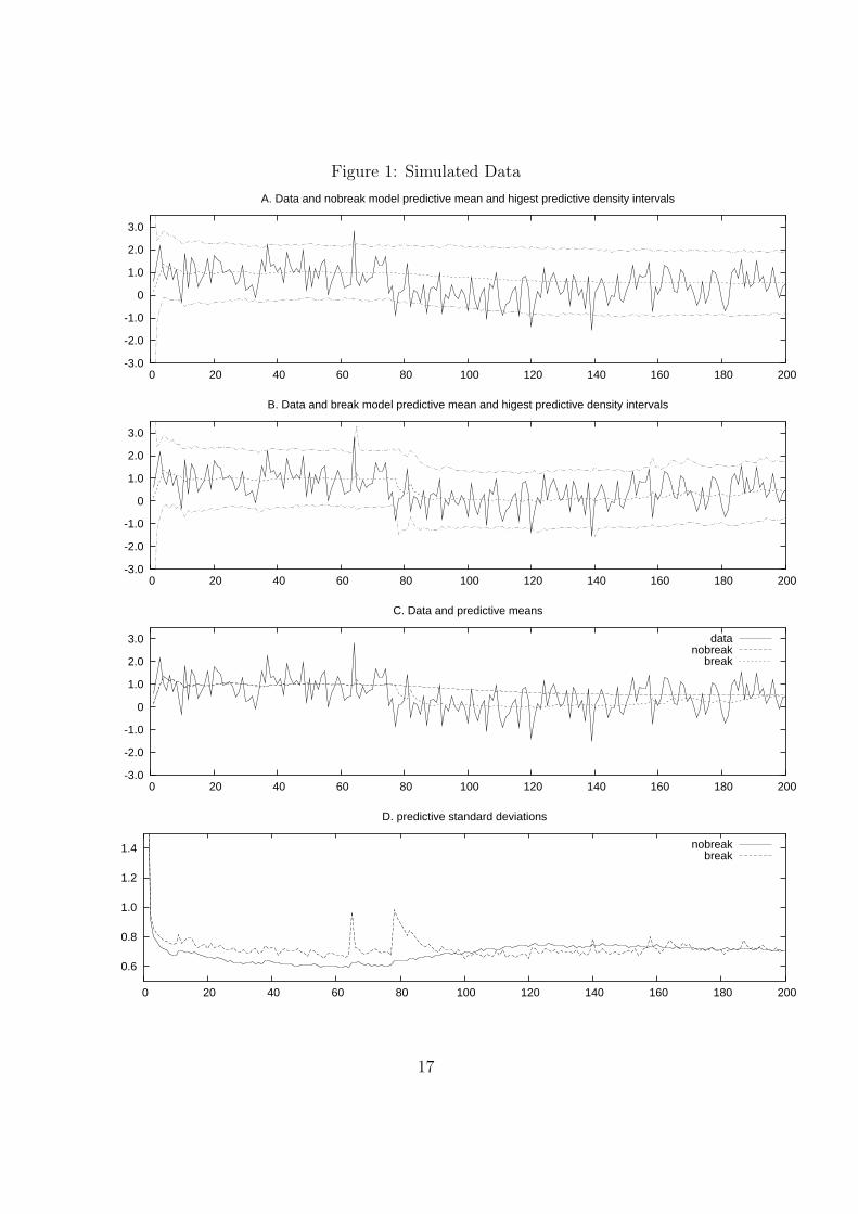
Figure 1: Simulated Data

-3.0

-2.0

-1.0

0

1.0

2.0

3.0

0 20 40 60 80 100 120 140 160 180 200

A. Data and nobreak model predictive mean and higest predictive density intervals

-3.0

-2.0

-1.0

0

1.0

2.0

3.0

0 20 40 60 80 100 120 140 160 180 200

B. Data and break model predictive mean and higest predictive density intervals

-3.0

-2.0

-1.0

0

1.0

2.0

3.0

0 20 40 60 80 100 120 140 160 180 200

C. Data and predictive means

datanobreak

break

0.6

0.8

1.0

1.2

1.4

0 20 40 60 80 100 120 140 160 180 200

D. predictive standard deviations

nobreakbreak

17

E. M

odel Probabilities

0 20

40 60

80 100

120 140

160 180

200

Tim

e

0 20

40 60

80 100

120 140

160 180

200

Model, M

i

0

0.1

0.2

0.3

0.4

0.5

0.6

0.7

0.8

0.9 1

Probability

18

Figure 2: Real GDP Growth Rates

-4.0

-2.0

0

2.0

4.0

6.0

1950 1960 1970 1980 1990 2000


-4.0

-2.0

0

2.0

4.0

6.0

1950 1960 1970 1980 1990 2000


-4.0

-2.0

0

2.0

4.0

6.0

1950 1960 1970 1980 1990 2000

C. Data and predictive means

datanobreak

break

0.5

1.0

1.5

2.0

1950 1960 1970 1980 1990 2000

D. predictive standard deviations

nobreakbreak

19

E. M

odel Probabilities

1950

1960

1970

1980

1990

2000

Tim

e

1950

1960

1970

1980

1990

2000

Model, M

i

0

0.1

0.2

0.3

0.4

0.5

0.6

0.7

0.8

0.9 1

Probability

20

Figure 3: Model Probabilities

0

0.05

0.1

0.15

0.2

1950 1960 1970 1980 1990 2000Model, Mi

Figure 4: Moments through Time

-0.2 0

0.2 0.4 0.6 0.8

1 1.2 1.4 1.6 1.8

2

1950 1960 1970 1980 1990 2000

A. Unconditional Mean

0.2 0.4 0.6 0.8

1 1.2 1.4 1.6 1.8

2 2.2

1950 1960 1970 1980 1990 2000

B. Unconditional Variance

21

Figure 5: Inflation, h=4

-4.0

-2.0

0

2.0

4.0

6.0

1950 1960 1970 1980 1990 2000


-4.0

-2.0

0

2.0

4.0

6.0

1950 1960 1970 1980 1990 2000


0.5

1.0

1.5

1950 1960 1970 1980 1990 2000

C. predictive standard deviations

nobreakbreak

22

D. M

odel Probabilities

1950

1960

1970

1980

1990

2000

Tim

e

1950

1960

1970

1980

1990

2000

Model, M

i

0

0.2

0.4

0.6

0.8 1

Probability

23

Figure 6: Parameter Estimates through Time, h=4

-1.5-1

-0.5

0 0.5

1 1.5

2 2.5

3

1950 1960 1970 1980 1990 2000

A

β1

-0.6

-0.4

-0.2

0

0.2

0.4

0.6

0.8

1950 1960 1970 1980 1990 2000

B

β2

-0.2

-0.1

0

0.1

0.2

0.3

0.4

0.5

1950 1960 1970 1980 1990 2000

C

β3β4

0

0.1

0.2

0.3

0.4

0.5

0.6

1950 1960 1970 1980 1990 2000

D

σ2

24

References

Andrews, D. W. K. (1993): “Tests for Parameter Instability and Structural Changewith Unknown Change Point,” Econometrica, 61, 821–856.

(2003): “End-of-Sample Instability Tests,” Econometrica, 71(6), 1661–1694.

Andrews, D. W. K., I. Lee, and W. Ploberger (1996): “Optimal ChangepointTests for Normal Linear Regression Model,” Journal of Econometrics, 70, 9–38.

Bai, J., and P. Perron (1998): “Estimating and Testing Linear Models with MultipleStructural Breaks,” Econometrica, 66(1), 47–78.

Carlin, B., A. E. Gelfand, and A. F. M. Smith (1992): “Hierarchical BayesianAnalysis of Changepoint Problems,” Applied Statistics, (41), 389–405.

Chib, S. (1995): “Marginal Likelihood from the Gibbs Sampler,” Journal of the Amer-ican Statistical Association, 90, 1313–1321.

(1998): “Estimation and Comparison of Multiple Change Point Models,” Jour-nal of Econometrics, 86, 221–241.

Chib, S. (2001): “Markov Chain Monte Carlo Methods: Computation and Inference,”in Handbook of Econometrics, ed. by Heckman, and Leamer. Elsevier Science.

Dufour, J. M., E. Ghysels, and A. Hall (1994): “Generalized Predictive Testsand Structural Change Analysis in Econometrics,” International Economic Review,35, 199–229.

Gelfand, A., and D. Dey (1994): “Bayesian Model Choice: Asymptotics and ExactCalculations,” B, 56, 501–514.

Geweke, J. (1995): “Bayesian Comparison of Econometric Models,” University ofIowa.

Geweke, J. (1998): “Comment on Real and Spurious Long-Memory Proporties ofStock Market Data,” Journal of Business & Economic Statistics, 16(3), 269–271.

Ghysels, E., A. Guay, and A. Hall (1997): “Predictive Tests for Structural Changewith Unknown Breakpoint,” Journal of Econometrics, 82, 209–233.

Ghysels, E., and A. Hall (1990): “A Test for Structural Stability of Euler Con-ditions Parameters Estimated vis the Generalized Methods of Moments Estimator,”International Economic Review, 31, 355–364.

Hamilton, J. D. (1989): “A New Approach to the Economic Analysis of Non-stationary Time Series and the Business Cycle,” Econometrica, 57, 357–384.

25

Hansen, B. E. (1992): “Tests for Parameter Instability in Regressions with I(1) Pro-cesses,” Journal of Business & Economic Statistics, 10, 321–336.

Inclan, C. (1994): “Detection of Multiple Changes of Variance using Posterior Odds,”Journal of Business & Economic Statistics, 11(3), 289–300.

Kim, C. J., and C. R. Nelson (1999): “Has the U.S. Economy Become More Stable?A Bayesian Approach Based on a Markov-Switching Model of the Business Cycle,”Review of Economics and Statistics, 81, 608–616.

Kim, C. J., C. R. Nelson, and J. Piger (2004): “The Less-Volatile U.S. Economy”A Bayesian Investigation of Timing, Breath, and Potential Explanations,” Journal ofBusiness & Economic Statistics, 22(1), 80–93.

Koop, G. (2003): Bayesian Econometrics. Wiley, Chichester, England.

Koop, G., and S. Potter (2001): “Are Apparent Findings of Nonlinearity Due toStructural Instability in Economic Time Series?,” Econometrics Journal, 4, 37–55.

McConnell, M. M., and G. P. Perez-Quiros (2000): “Output Fluctuations inthe United States: What Has Changed Since the Early 1980s?,” American EconomicReview, 90(1464-1476).

McCulloch, R. E., and R. Tsay (1993): “Bayesian Inference and Prediction forMean and Variance Shilts in Autoregressive Time Series,” Journal of the AmericanStatistical Association, 88, 968–978.

Newton, M. A., and A. Raftery (1994): “Approximate Bayesian inference by theweighted likelihood bootstrap (with Discussion).,” B, 56, 3–48.

Nicholls, D. F., and A. R. Pagan (1985): “Varying Coefficient Regression,” inHandbook of Statistics, ed. by Hannan, Krishnaiah, and Rao. North Holland.

Pasaran, M. H., D. Pettenuzzo, and A. Timmermann (2004): “ForecastingTime Series Subject to Multiple Structural Breaks,” Cambridge Working Papers inEconomics, 433.

Robert, C. P., and G. Casella (1999): Monte Carlo Statistical Methods. Springer,New York.

Stock, J., and M. Watson (1996): “Evidence of Structural Instability in Macroeco-nomic Time Series Relations,” Journal of Business & Economic Statistics, 14, 11–30.

(2002): “Has the Business Cycle Changed and Why?,” NBER MacroeconomicsAnnual, pp. 159–218.

26

Stock, J. H., and M. W. Watson (1999): “Forecasting Inflation,” Journal of Mon-etary Economics, 44, 293–335.

Wang, J., and E. Zivot (2000): “A Bayesian Time Series Model of Multiple StructuralChanges in Level, Trend, and Variance,” Journal of Business & Economic Statistics,18(3), 374–386.

Zellner, A. (1986): “Bayesian Estimation and Prediction using Asymmetric LossFunctions,” Journal of the American Statistical Association, 81, 446–451.

27

Learning, Forecasting and Structural Breaks1

Documents

Transcript of Learning, Forecasting and Structural Breaks1