Learning Financial Market Datawith Recurrent Autoencoders and TensorFlow.

Steven Hutt steven.c.hutt@gmail.comJuly 28, 2016

TensorFlow London Meetup

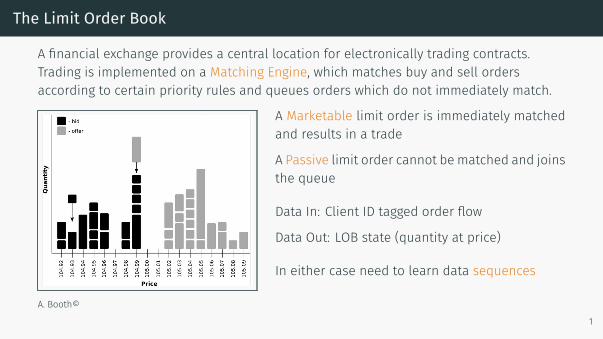
The Limit Order Book

A financial exchange provides a central location for electronically trading contracts.Trading is implemented on a Matching Engine, which matches buy and sell ordersaccording to certain priority rules and queues orders which do not immediately match.

A. Booth©

A Marketable limit order is immediately matchedand results in a trade

A Passive limit order cannot be matched and joinsthe queue

Data In: Client ID tagged order flow

Data Out: LOB state (quantity at price)

In either case need to learn data sequences

1

Learning Sequences with RNNs

In a Recurrent Neural Network there are nodes which feedback on themselves. Belowxt ∈ Rnx , ht ∈ Rnh and zt ∈ Rnz , for t = 1, 2, . . . , T. Each node is a vector or 1-dim array.

..

output

.state .

input

.

zt

.ht.

xt

.

Whx

. Whh.

Wzh

. h0.

z1

.

z2

.

z3

. h1. h2. h3.

x1

.

x2

.

x3

.

zT

. hT.

xT

.

· · ·

. · · ·.

· · ·

The RNN is defined by update equations:

ht+1 = f(Whhht +Whxxt + bh), zt = g(Wyhht + bz).

where Wuv ∈ Rnu×nv and bu ∈ Rnu are the RNN weights and biases respectively. Thefunctions f and g are generally nonlinear.

2

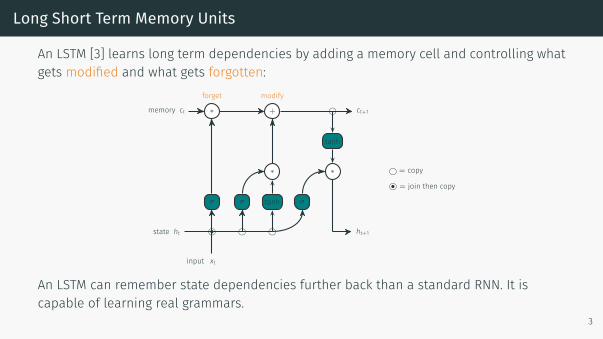
Long Short Term Memory Units

An LSTM [3] learns long term dependencies by adding a memory cell and controlling whatgets modified and what gets forgotten:

..memory ct .

state ht

.∗.forget

. +.modify

.

σ

.

σ

.

tanh

.

σ

.

∗

.

∗

.

tanh

.

•

.

⃝

.

⃝

.

⃝

.. ⃝.. ct+1.

ht+1

.

xt

.

input

.

⃝

.

= copy

.

•

.

⃝

.

= join then copy

An LSTM can remember state dependencies further back than a standard RNN. It iscapable of learning real grammars.

3

Unitary RNNs

The behaviour of the LSTM can be difficult to analyse.

An alternative approach [1] is to ensure there are no contractive directions, that isrequire Whh ∈ U(n), the space of unitary matrices.

This preserves the simple form of an RNN but ensures the state dependencies go furtherback in the sequence.A key problem is that gradient descent does not preservethe unitary property:

x ∈ U(n) 7→ x+ λυ /∈ U(n)

The solution in [1] is to choose Whh from asubset generated by parametrized unitarymatrices:

Whh = D3R2F−1D2ΠR1FD1.

Here D is diagonal, R is a reflection, F is the Fourier trans-form and Π is a permutation. 4

RNNs as Programs addressing External Memory

RNNs are Turing complete but the theoretical capabilities are not matched in practicedue to training inefficiencies.

The Neural Turing Machine emulates a differentiable Turing Machine by adding externaladdressable memory and using the RNN state as a memory controller [2].

..

Input xt

.

Output yt

.RNN Controller.RNN Controller.RNN Controller.

Read Heads

.

Write Heads

.

Memory

.

ml

.

ml

Vanila NTM Architecture

NTM equivalent 'code'initialise: move head to start locationwhile input delimiter not seen do

receive input vectorwrite input to head locationincrement head location by 1

end whilereturn head to start locationwhile true do

read output vector from head locationemit outputincrement head location by 1

end while 5

Deep RNNs

..

out

.

L3

.

L2

.L1 .

in

.

zt

.

h3t

.

h2t

.h1t.

xt

.

Wh1x

. Wh1h1

.

Wh2h2

.

Wh3h3

.

h1t

.

h2t

.

Wzh3

.

h30

.

h20

. h10.

z1

.

z2

.

z3

.

h31

.

h32

.

h33

.

h21

.

h22

.

h23

. h11. h12. h13.

x1

.

x2

.

x3

.

zT

.

h3T

.

h2T

. h1T.

xT

.

· · ·

.

· · ·

.

· · ·

. · · ·.

· · ·

The input to hidden layer Li is the state hi−1 of hidden layer Li−1. Deep RNNs can learn atdifferent time scales.

6

Autoencoders

The more regularities there are in data the more it can be compressed. The morewe are able to compress the data, the more we have learned about the data.

(Grünwald, 1998)

..

x1

.

x2

.

x3

.

x4

.

x5

.

x6

.

h11

.

h12

.

h13

.

h14

.

h21

.

h22

.

h31

.

h32

.

h33

.

h34

.

y1

.

y2

.

y3

.

y4

.

y5

.

y6

.

input

.

code

.

reconstruct

.

encode

.

decode

.Wh1x

.Wh2h1

.Wh3h2

.Wyh3

Autoencoder7

Recurrent Autoencoders

.. he0. he1. he2. he3.

x1

.

x2

.

x3

. heT.

xT

. · · ·.

· · ·

. hd0.

z1

.

z2

.

z3

. hd1. hd2. hd3.

z0

.

z1

.

z2

.

zT

. hdT.

zT−1

.

· · ·

. · · ·.

· · ·

. =

encoder decoder

A Recurrent Autoencoder is trained to output a reconstruction z of the the inputsequence x. All data must pass through the narrow heT . Compression between input andoutput forces pattern learning.

8

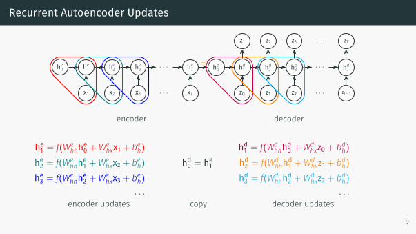
Recurrent Autoencoder Updates

.. he0. he1. he2. he3.

x1

.

x2

.

x3

. heT.

xT

. · · ·.

· · ·

................ hd0.

z1

.

z2

.

z3

. hd1. hd2. hd3.

z0

.

z1

.

z2

.

zT

. hdT.

zT−1

.

· · ·

. · · ·.

· · ·

. =...............

encoder decoder

he1 = f(Wehhhe0 +We

hxx1 + beh)he2 = f(We

hhhe1 +Wehxx2 + beh)

he3 = f(Wehhhe2 +We

hxx3 + beh)· · ·

encoder updates

hd0 = heT

copy

hd1 = f(Wdhhhd0 +Wd

hxz0 + bdh)hd2 = f(Wd

hhhd1 +Wdhxz1 + bdh)

hd3 = f(Wdhhhd2 +Wd

hxz2 + bdh)· · ·

decoder updates

9

Easy RNNs with TensorFlow VariableScope

def linear(in_array, out_size):in_size = in_array.get_shape()# creates or returns a variableW = vs.get_variable(shape=[in_size, out_size], name='W')# out_array = in_array * Wout_array = math_ops.matmul(in_array, W)return out_array

with tf.variable_scope('encoder_0') as scope:# creates variable encoder_0/Wout_array_1 = linear(in_array_0, out_size_1)

# error: encoder_0/W already exists# out_array_2 = linear(out_array_1, out_size_2)

# reuse encoder_0/Wscope.reuse_variables()out_array_2 = linear(out_array_1, out_size_2)

10

TensorFlow encoder

with tf.variable_scope('encoder_0') as scope:for t in range(1, seq_len):

# placeholder for input data at time txs_0_enc[t] = tf.placeholder(shape=[None, nx_enc])# encoder update at time ths_0_enc[t] = lstm_cell_l0_enc(xs_0_enc[t], hs_0_enc[t-1])scope.reuse_variables() 11

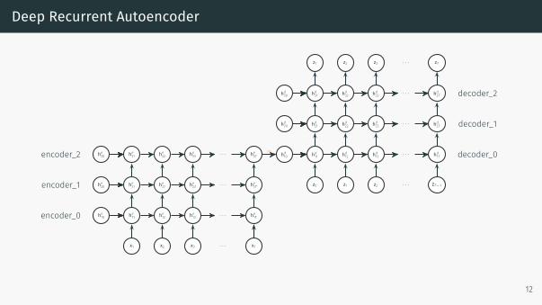
Deep Recurrent Autoencoder

...

encoder_2

.

encoder_1

.encoder_0.

he30

.

he20

. he10.

he31

.

he32

.

he33

.

he21

.

he22

.

he23

. he11. he12. he13.

x1

.

x2

.

x3

.

he3T

.

he2T

. he1T.

xT

.

· · ·

.

· · ·

. · · ·.

· · ·

.

decoder_2

.

decoder_1

.

decoder_0

.

hd30

.

hd20

.

hd10

.

hd31

.

hd32

.

hd33

.

hd21

.

hd22

.

hd23

.

hd11

.

hd12

.

hd13

.

z1

.

z2

.

z3

.

z0

.

z1

.

z2

.

hd3T

.

hd2T

.

hd1T

.

zT−1

.

zT

.

· · ·

.

· · ·

.

· · ·

.

· · ·

.

· · ·

.

=

12

TensorFlow Deep Recurrent AutoEncoder

with tf.variable_scope('encoder_0') as scope:for t in range(1, seq_len):

# placeholder for input dataxs_0_enc[t] = tf.placeholder(shape=[None, nx_enc])hs_0_enc[t] = lstm_cell_l0_enc(xs_0_enc[t], hs_0_enc[t-1])scope.reuse_variables()

with tf.variable_scope('encoder_1') as scope:for t in range(1, seq_len):

# encoder_1 input is encoder_0 hidden statexs_1_enc[t] = hs_0_enc[t]hs_1_enc[t] = lstm_cell_l1_enc(xs_1_enc[t], hs_1_enc[t-1])scope.reuse_variables()

with tf.variable_scope('encoder_2') as scope:for t in range(1, seq_len):

# encoder_2 input is encoder_1 hidden statexs_2_enc[t] = hs_1_enc[t]hs_2_enc[t] = lstm_cell_l2_enc(xs_2_enc[t], hs_2_enc[t-1])scope.reuse_variables() 13

Variational Autoencoder

We assume the market data {xk} is sampled from a probability distribution with a 'small'number of latent variables h.

Assume pθ(x,h) = pθ(x |h)pθ(h) where θ are

weights of a NN/RNN. Then

pθ(x) =∑h

pθ(x |h)pθ(h)

Train network to minimize

Lθ({xk}) = minθ

∑k

− log(pθ(xk)).

Compute pθ(h | x) and cluster.

But pθ(h | x) is intractable!

..h.

x

. pθ(h).

pθ(x)

. prior.

likelihood

.

marginal

.

posterior

.

p(x | h)

.

pθ(h | x)

14

Variational Inference

Variational Inference learns an NN/RNN approximation qϕ(h | x) to pθ(h | x) duringtraining.

Think of qϕ as encoder and pθ decoder networks: an autoencoder.

Then logpθ(xk) ≥ Lθ,ϕ(xk) where

Lθ,ϕ(xk) = −DKL(qϕ(h | xk)||pθ(h))︸ ︷︷ ︸regularization term

+ Eqϕ(logpθ(xk |h))︸ ︷︷ ︸reconstruction term

is the variational lower bound.

Reconstruction term = log-likelihood wrt qϕ

Regularization term = target prior on encoder

..h.

x

. pθ(h).

pθ(x)

. prior.

likelihood

.

marginal

.

approx

.

pθ(x | h)

.

qϕ(h | x)

15

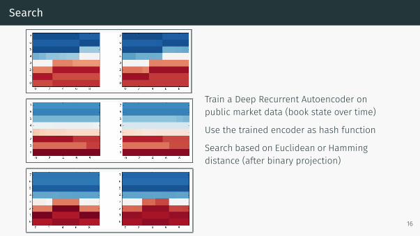
Search

Train a Deep Recurrent Autoencoder onpublic market data (book state over time)

Use the trained encoder as hash function

Search based on Euclidean or Hammingdistance (after binary projection)

16

Classify

EUR vs AUD

Train a Variational Recurrent Autoencoder with Gaus-sian prior on public market data

Include two contracts: EUR and AUD in training data

Use trained encoder to infer Gaussian means fromtraining data

17

Predict

Train an LSTM on sequences of states of the LOB to predict changes in best bid.

Target data: change in best bid over time t→ t+ 1.

LSTM output: zt = softmax distribution for best bid moves (−1, 0,+1) over time t→ t+ 1.

It's tough to make predictions, especially about the future.

target

predict

18

Questions?

18

References

M. Arjovsky, A. Shah, and Y. Bengio.Unitary evolution recurrent neural networks.arXiv:1511.06464v4, 2016.A. Graves, G. Wayne, and I. Danihelka.Neural turing machines.arXiv:1410.5401v2, 2014.S. Hochreiter and J. Schmidhuber.Long short term memory.Neural Computation, 9:1735--1780, 1997.

19