Learning Decision Trees - Peoplerussell/classes/cs194/f11... · Outline ♦Decision tree models...

Learning Decision Trees

CS194-10 Fall 2011 Lecture 8

CS194-10 Fall 2011 Lecture 8 1

Outline

♦ Decision tree models

♦ Tree construction

♦ Tree pruning

♦ Continuous input features


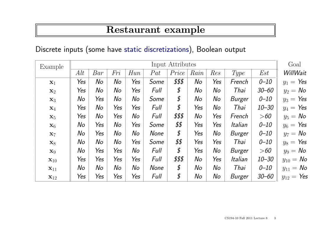
Restaurant example

Discrete inputs (some have static discretizations), Boolean output

Example Input Attributes Goal

Alt Bar Fri Hun Pat Price Rain Res Type Est WillWait

x1 Yes No No Yes Some $$$ No Yes French 0–10 y1 = Yes

x2 Yes No No Yes Full $ No No Thai 30–60 y2 = No

x3 No Yes No No Some $ No No Burger 0–10 y3 = Yes

x4 Yes No Yes Yes Full $ Yes No Thai 10–30 y4 = Yes

x5 Yes No Yes No Full $$$ No Yes French >60 y5 = No

x6 No Yes No Yes Some $$ Yes Yes Italian 0–10 y6 = Yes

x7 No Yes No No None $ Yes No Burger 0–10 y7 = No

x8 No No No Yes Some $$ Yes Yes Thai 0–10 y8 = Yes

x9 No Yes Yes No Full $ Yes No Burger >60 y9 = No

x10 Yes Yes Yes Yes Full $$$ No Yes Italian 10–30 y10 = No

x11 No No No No None $ No No Thai 0–10 y11 = No

x12 Yes Yes Yes Yes Full $ No No Burger 30–60 y12 = Yes


Decision trees

Popular representation for hypotheses, even among humans!E.g., here is the “true” tree for deciding whether to wait:

No Yes

No Yes

No Yes

No Yes

No Yes

No Yes

None Some Full

>60 30!60 10!30 0!10

No YesAlternate?

Hungry?

Reservation?

Bar? Raining?

Alternate?

Patrons?

Fri/Sat?

WaitEstimate?F T

F T

T

T

F T

TFT

TF


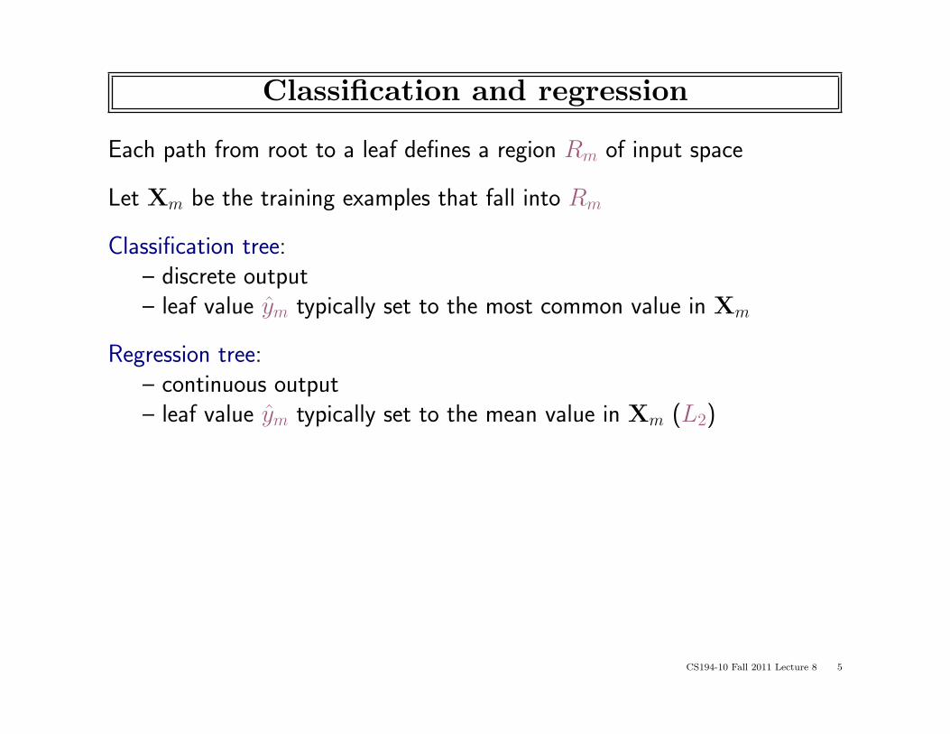
Classification and regression

Each path from root to a leaf defines a region Rm of input space

Let Xm be the training examples that fall into Rm

Classification tree:– discrete output– leaf value ym typically set to the most common value in Xm

Regression tree:– continuous output– leaf value ym typically set to the mean value in Xm (L2)


Discrete and continuous inputs

Simplest case: discrete inputs with small ranges (e.g., Boolean)⇒ one branch for each value; attribute is “used up” (“complete split”)

For continuous attribute, test is Xj > c for some split point c⇒ two branches, attribute may be split further in each subtree

Also split large discrete ranges into two or more subsets


Expressiveness

Discrete-input, discrete-output case:– Decision trees can express any function of the input attributes.– E.g., for Boolean functions, truth table row → path to leaf:

FT

A

B

F T

B

A B A xor BF F FF T TT F TT T F

F

F F

T

T T

Continuous-input, continuous-output case:– Can approximate any function arbitrarily closely

Trivially, there is a consistent decision tree for any training setw/ one path to leaf for each example (unless f nondeterministic in x)but it probably won’t generalize to new examples

Need some kind of regularization to ensure more compact decision trees


Digression: Hypothesis spaces

How many distinct decision trees with n Boolean attributes??




= number of Boolean functions




= number of Boolean functions= number of distinct truth tables with 2n rows




= number of Boolean functions= number of distinct truth tables with 2n rows = 22n





E.g., with 6 Boolean attributes, there are 18,446,744,073,709,551,616 trees






How many purely conjunctive hypotheses (e.g., Hungry ∧ ¬Rain)??






How many purely conjunctive hypotheses (e.g., Hungry ∧ ¬Rain)??

Each attribute can be in (positive), in (negative), or out⇒ 3n distinct conjunctive hypotheses



More expressive hypothesis space– increases chance that target function can be expressed– increases number of hypotheses consistent w/ training set⇒ many consistent hypotheses have large test error⇒ may get worse predictions

22nhypotheses ⇒ all but an exponentially small fraction will require O(2n)

bits to describe in any representation (decision trees, SVMs, English, brains)

Conversely, any given hypothesis representation can provide compact de-scriptions for only an exponentially small fraction of functions

E.g., decision trees are bad for “additive threshold”-type functions such as“at least 6 of the 10 inputs must be true,” but linear separators are good


Decision tree learning

Aim: find a small tree consistent with the training examples

Idea: (recursively) choose “most significant” attribute as root of (sub)tree

function Decision-Tree-Learning(examples,attributes,parent examples)

returns a tree

if examples is empty then return Plurality-Value(parent examples)

else if all examples have the same classification then return the classification

else if attributes is empty then return Plurality-Value(examples)

else

A← argmaxa ∈ attributes Importance(a, examples)

tree← a new decision tree with root test A

for each value vk of A do

exs←{e : e∈ examples and e.A = vk}subtree←Decision-Tree-Learning(exs,attributes−A, examples)

add a branch to tree with label (A = v k) and subtree subtree

return tree


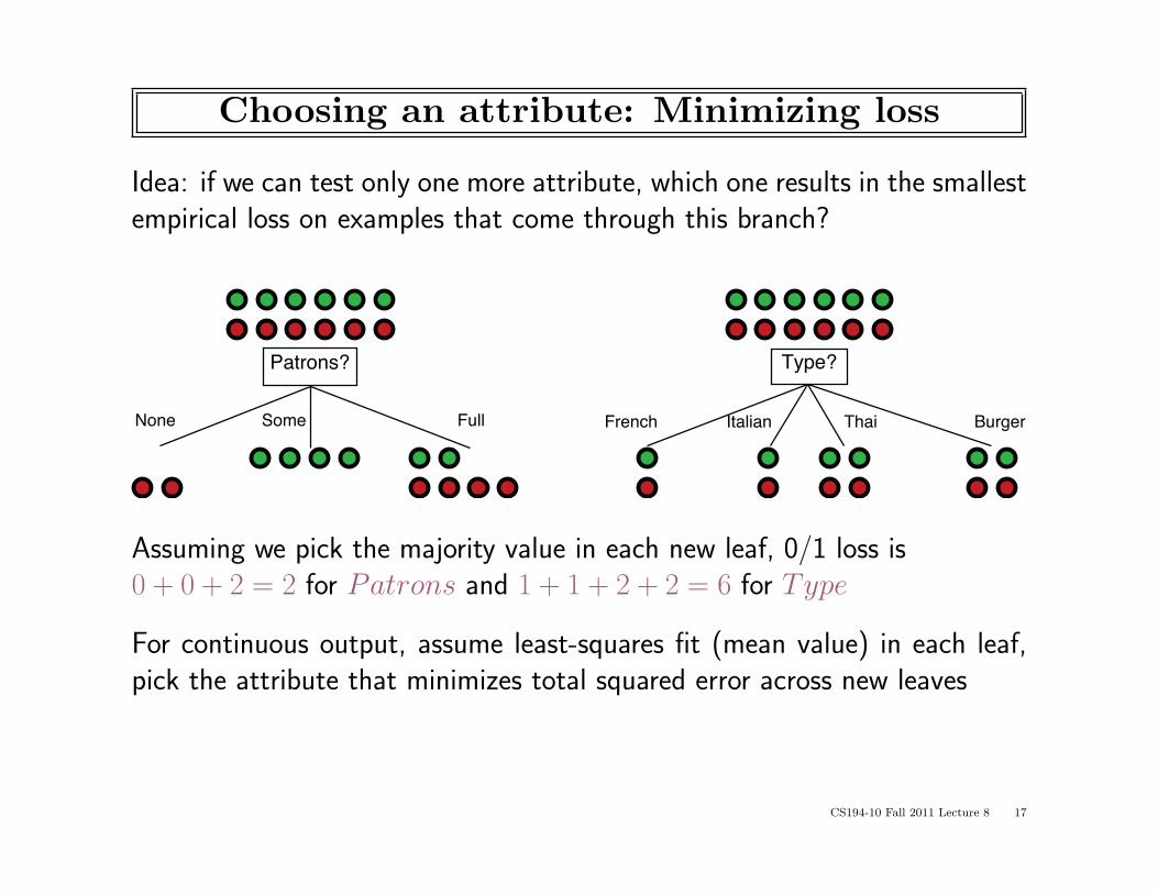
Choosing an attribute: Minimizing loss

Idea: if we can test only one more attribute, which one results in the smallestempirical loss on examples that come through this branch?

None Some Full

Patrons?

French Italian Thai Burger

Type?

Assuming we pick the majority value in each new leaf, 0/1 loss is0 + 0 + 2 = 2 for Patrons and 1 + 1 + 2 + 2 = 6 for Type

For continuous output, assume least-squares fit (mean value) in each leaf,pick the attribute that minimizes total squared error across new leaves


Choosing an attribute: Information gain

Idea: measure the contribution the attribute makes to increasing the “purity”of the Y -values in each subset of examples

None Some Full

Patrons?


Type?

Patrons is a better choice—gives information about the classification(also known as reducing entropy of distribution of output values)


Information

Information answers questions

The more clueless I am about the answer initially, the more information iscontained in the answer

Scale: 1 bit = answer to Boolean question with prior 〈0.5, 0.5〉

Information in an answer when prior is 〈P1, . . . , Pn〉 is

H(〈P1, . . . , Pn〉) = Σni = 1 − Pi log2 Pi

(also called entropy of the prior)

Convenient notation: B(p) = H(〈p, 1− p〉)


Information contd.

Suppose we have p positive and n negative examples at the root⇒ B(p/(p + n) bits needed to classify a new example

E.g., for 12 restaurant examples, p = n = 6 so we need 1 bit

An attribute splits the examples E into subsets Ek, each of which (we hope)needs less information to complete the classification

Let Ek have pk positive and nk negative examples⇒ B(pk/(pk + nk) bits needed to classify a new example⇒ expected number of bits per example over all branches is

Σipi + ni

p + nB(pk/(pk + nk))

For Patrons, this is 0.459 bits, for Type this is (still) 1 bit

⇒ choose the attribute that minimizes the remaining information needed


Empirical loss vs. information gain

Information gain tends to be less greedy:– Suppose Xj splits a 10/6 parent into 2/0 and 8/6 leaves– 0/1 loss is 6 for parent, 6 for children: “no progress”– 0/1 loss is still 6 with 4/0 and 6/6 leaves! – Information gain is 0.2044

bits: we have “peeled off” an easy category

Most experimental investigations indicate that information gainleads to better results (smaller trees, better predictive accuracy)


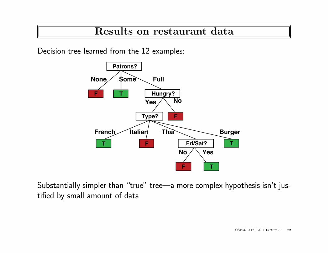
Results on restaurant data

Decision tree learned from the 12 examples:

No YesFri/Sat?

None Some FullPatrons?

No YesHungry?

Type?


F T

T F

F

T

F T

Substantially simpler than “true” tree—a more complex hypothesis isn’t jus-tified by small amount of data


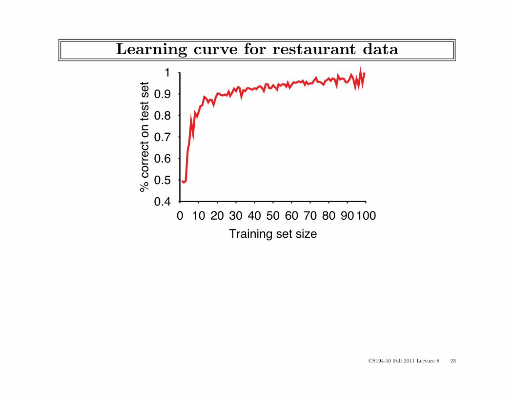
Learning curve for restaurant data

0.40.50.60.70.80.9

1

0 10 20 30 40 50 60 70 80 90 100

% co

rrect

on te

st se

t

Training set size


Pruning

Tree grows until it fits the data perfectly or runs out of attributes

In the non-realizable case, will severely overfit

Pruning methods trim tree back, removing “weak” tests

A test is weak if its ability to separate +ve and -ve is notsignificantly different from that of a completely irrelevant attribute

E.g., Xj splits a 4/8 parent into 2/2 and 2/6 leaves; gain is 0.04411 bits.How likely is it that randomly assigning the examples to leaves of the samesize leads to a gain of at least this amount?

Test the deviation from 0-gain split using χ2-squared statistic,prune leaves of nodes that fail the test, repeat until done.Regularization parameter is the χ2 threshold (10%, 5%, 1%, etc.)


Optimal splits for continuous attributes

Infinitely many possible split points c to define node test Xj > c ?


Optimal splits for continuous attributes

Infinitely many possible split points c to define node test Xj > c ?

No! Moving split point along the empty space between two observed valueshas no effect on information gain or empirical loss; so just use midpoint

Xj

c1 c2

Moreover, only splits between examples from different classescan be optimal for information gain or empirical loss reduction

Xj

c2c1


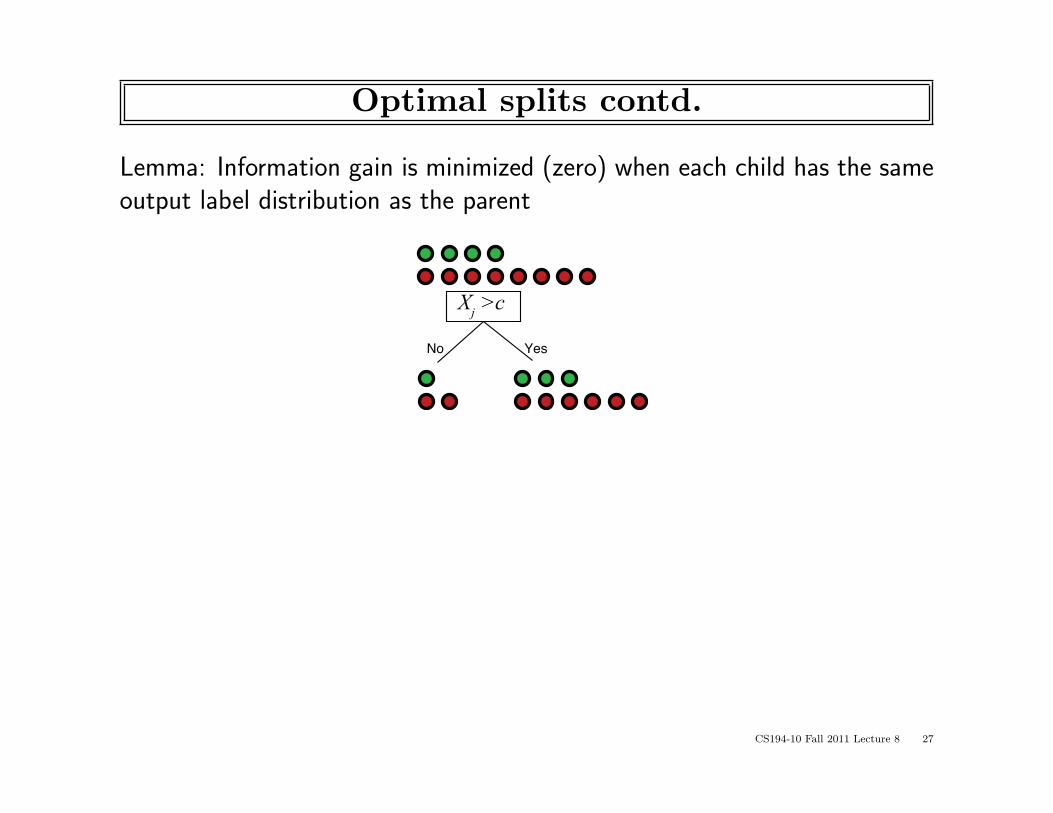
Optimal splits contd.

Lemma: Information gain is minimized (zero) when each child has the sameoutput label distribution as the parent

No Yes

Xj >c


Optimal splits contd.

Lemma: if c splits Xj between two +ve examples, andexamples to the left of c are more +ve than the parent distribution, then

– examples to the right are are more -ve than the parent distribution,– moving c right by one takes children further from parent distribution,– and information gain necessarily increases

Xj

c2c1

No Yes

Xj >c1No Yes

Xj >c2

Gain for c1: B( 412)−

(412B(2

4) + 812B(2

8))

= 0.04411 bits

Gain for c2: B( 412)−

(512B(3

5) + 712B(1

7))

= 0.16859 bits


Optimal splits for discrete attributes

A discrete attribute may have many possible values– e.g., ResidenceState has 50 values

Intuitively, this is likely to result in overfitting;extreme case is an identifier such as SS#.

Solutions:– don’t use such attributes– use them and hope for the best– group values by hand (e.g., NorthEast, South, MidWest, etc.)– find best split into two subsets–but there are 2K subsets!


Optimal splits for discrete attributes contd.

The following algorithm gives an optimal binary split:

Let pjk be proportion of +ve examplesin the set of examples that have Xj = xjk

Order the values xjk by pjk

Choose the best split point just as for continuous attributes

E.g., pj,CA = 7/10, pj,NY = 4/10, pj,TX = 5/20, pj,IL = 3/20;ascending order is IL, TX, NY , CA; 3 possible split points.


Additional tricks

Blended selection criterion: info gain near root, empirical loss near leaves

“Oblique splits”: node test is a linear inequality wTx + b > 0

Full regressions at leaves: y(x) = (XT` X`)

−1XT` Y`

Cost-sensitive classification

Lopsided outputs: one class very rare (e.g., direct mail targeting)

Scaling up: disk-resident data


Summary

“Of all the well-known learning methods, decision trees come closest tomeeting the requirements for serving as an off-the-shelf procedure for datamining.” [Hastie et al.]

Efficient learning algorithm

Handle both discrete and continuous inputs and outputs

Robust against any monotonic input transformation, also against outliers

Automatically ignore irrelevant features: no need for feature selection

Decision trees are usually interpretable


Learning Decision Trees - Peoplerussell/classes/cs194/f11... · Outline ♦Decision tree models...

Documents

Transcript of Learning Decision Trees - Peoplerussell/classes/cs194/f11... · Outline ♦Decision tree models...