Learning Data System Components - MIT
129
Learning Data System Components 6.830 Lecture 11 Sivaprasad Sudhir, Kapil Vaidya Slides Courtesy: Prof. Tim Kraska
Transcript of Learning Data System Components - MIT

Learning Data System Components
6.830 Lecture 11
Sivaprasad Sudhir, Kapil Vaidya
Slides Courtesy: Prof. Tim Kraska

Building Blocks of Data Systems
• Indexes
• Joins
• Sorting
• Caching
• Hash Tables

An example
• Index all Integers from 100 to 1M
100 101 102 103 104 105 ... 1MData =
B-Tree?

An example
• Index all Integers from 100 to 1M
100 101 102 103 104 105 ... 1MData =
Data[key – 100]

An example
• What about even integers?
100 101 102 103 104 105 ... 1MData =
100 102 104 106 108 110 ... 1MData =
Data[(key – 100) / 2]
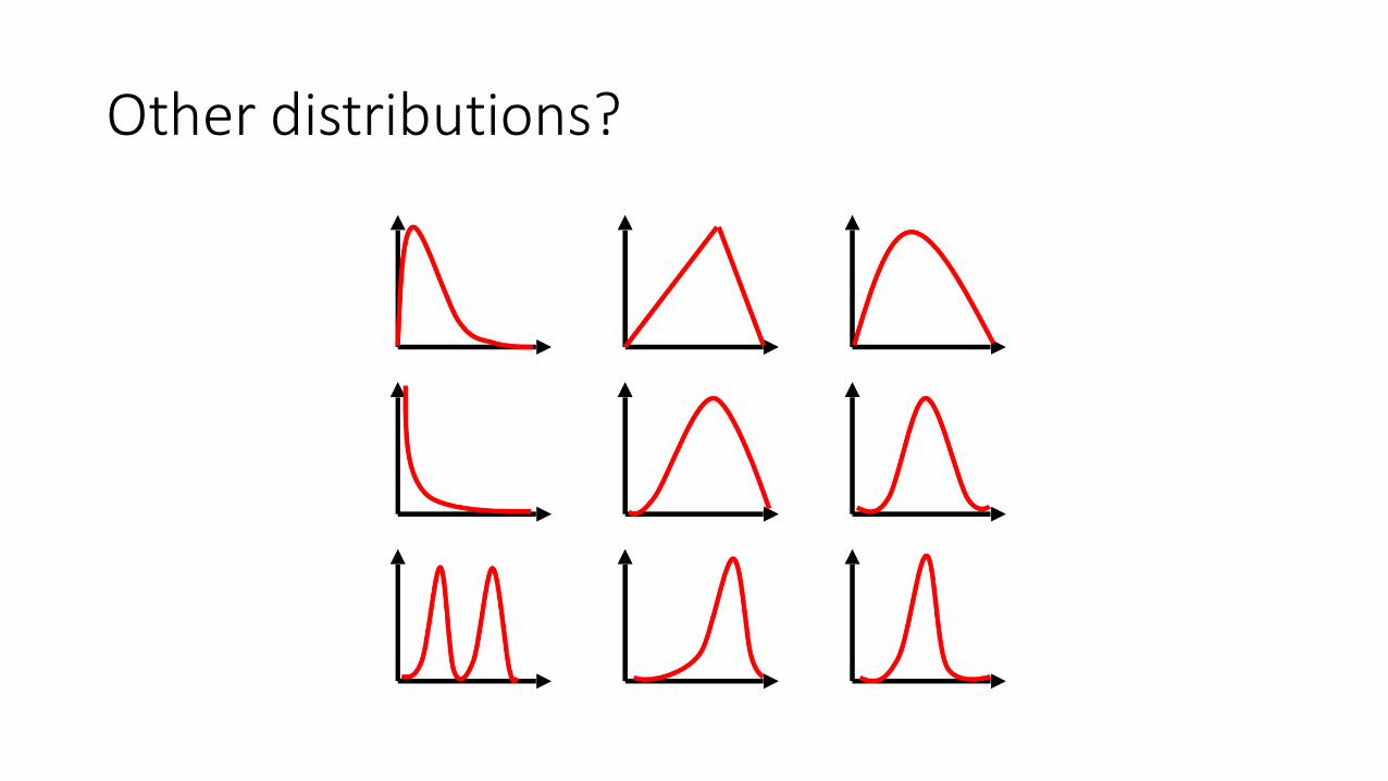
Other distributions?

Key Insight
• Traditional data structures make no assumption about data
• Optimized for worst case

• Building a system from scratch for every use case is not scalable
• What if we could learn the data distribution?
8

Setup
• In-memory
• Read only
9

B-Tree as a model
• Maps key to page
B-Tree
Pages

B-Tree as a model
• Maps key to pos
• Search between pos and pos + page size
B-Tree
Sorted Array
pos pos + page size

B-Tree as a model
• Model that predicts the position of a key within some error bounds
Sorted Array
pos pos + page size
Model

Index as a model
• Model maps key to pos
• Search in [pos – errmin, pos + errmax]
• errmin and errmax are known from training
Sorted Array
pos - errmin pos + errmax
Model

What is the model estimating?
• Predicting the position of a key
• Modeling the CDF of the keys
• pos = P(X <= key) * #keys
14
Sorted Array
pos - errmin pos + errmax
Model

What is the model estimating?
• Predicting the position of a key
• Modeling the CDF of the keys
• pos = P(X <= key) * #keys
= F(key) * #keys
15

LookUp(key)
• Use the CDF model to predict the position of the key
• pos = F(key) * #keys
• Scan from [pos – errmin, pos + errmax]
16
Key Idea
• When CPU cycles are cheap relative to memory accesses, compute-intensive function approximations can be beneficial for lookups
• ML models may be better at approximating some functions than existing data structures
• Power of continuous functions

Potential Advantages of Learned Models
• Smaller indexes
• Faster lookups
18

What Models?
• 200M web-server log records by timestamp-sorted
• 2-layer NN, 32 width, ReLU activated
• Prediction task: timestamp -> position within sorted array

Naïve Approach
20
250 ns ???

Naïve Approach
21
250 ns 80,000 ns
Problems
1. Tensorflow is designed for large models
2. B-Trees are very good at overfitting
3. B-Trees are cache-efficient
4. Search does not take advantage of the prediction

Precision gain per node

Last Mile Problem
24

Recursive Model Index (RMI)
floor(F1.1(key) * M2) = 0
floor(F2.1(key) * M3) = 1
floor(F3.2(key) * N) = pos
Fl.k - CDF of Ml.kMl – Number of models in level lN – Number of keys

Recursive Model Index (RMI)

Min-/Max-Error vs Average Error
27

Binary Search
28
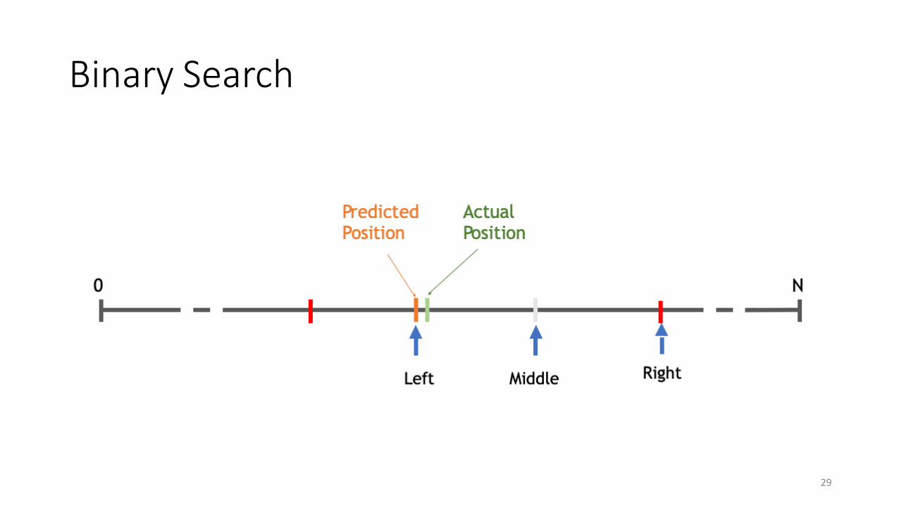
Binary Search
29

Binary Search
30

Exponential Search
31

Results
Ryan Marcus, Andreas Kipf, Alexander van Renen, Mihail Stoian, Sanchit Misra, Alfons Kemper, Thomas Neumann, and Tim Kraska. 2020. Benchmarking learned indexes. Proc. VLDB Endow. 14, 1 (September 2020), 1–13. DOI:https://doi.org/10.14778/3421424.3421425

Updates?
Ding, Jialin, et al. "ALEX: an updatable adaptive learned index." Proceedings of the 2020 ACM SIGMOD International Conference on Management of Data. 2020.
Slides Courtesy: Jialin Ding

• Why are inserts hard?
• How do B-Trees handle inserts?
34

ALEX
• Goals• Writes competitive with B+ Tree
• Reads faster than B+ Tree and Learned Index
• Index size smaller than B+ Tree and Learned Index
• Core structure• Dynamic tree structure
• Models
35

ALEX Core Ideas
Faster Reads Faster Writes Adaptiveness
1. Gapped Array ✔
2. Model-based Inserts ✔
3. Adaptive Tree Structure ✔ ✔ ✔
36

1. Gapped Array
37
1 2 3 4 5 6 7 8Dense Array

1. Gapped Array
38
1 2 3 4 5 6 7 8Dense Array
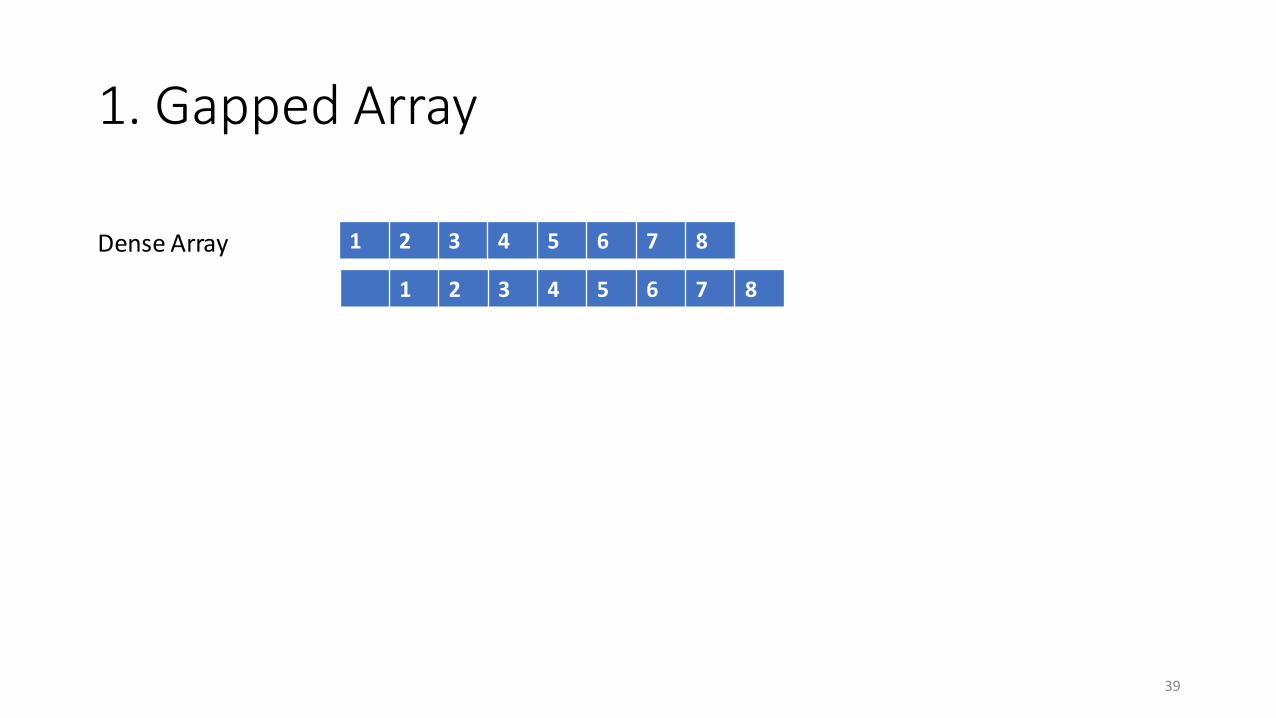
1. Gapped Array
39
1 2 3 4 5 6 7 8Dense Array
1 2 3 4 5 6 7 8

1. Gapped Array
40
1 2 3 4 5 6 7 8Dense Array
0 1 2 3 4 5 6 7 8

1. Gapped Array
41
Dense Array 0 1 2 3 4 5 6 7 8
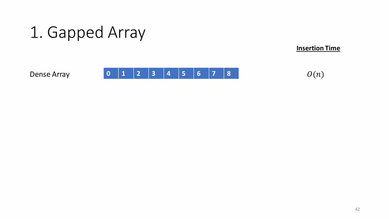
1. Gapped Array
42
Dense Array 𝑂(𝑛)
Insertion Time
0 1 2 3 4 5 6 7 8

1. Gapped Array
43
Dense Array 𝑂(𝑛)
Insertion Time
1 2 3 4 5 6 7 8B+ Tree Node
0 1 2 3 4 5 6 7 8

1. Gapped Array
44
Dense Array 𝑂(𝑛)
Insertion Time
1 2 3 4 5 6 7 8B+ Tree Node
0 1 2 3 4 5 6 7 8

1. Gapped Array
45
Dense Array 𝑂(𝑛)
Insertion Time
0 1 2 3 4 5 6 7 8B+ Tree Node
0 1 2 3 4 5 6 7 8

1. Gapped Array
46
Dense Array 𝑂(𝑛)
Insertion Time
0 1 2 3 4 5 6 7 8B+ Tree Node
0 1 2 3 4 5 6 7 8
𝑂(𝑛)

1. Gapped Array
47
Dense Array 𝑂(𝑛)
Insertion Time
0 1 2 3 4 5 6 7 8B+ Tree Node
0 1 2 3 4 5 6 7 8
𝑂(𝑛)
1 2 3 4 5 6 7 8Gapped Array

1. Gapped Array
48
Dense Array 𝑂(𝑛)
Insertion Time
0 1 2 3 4 5 6 7 8B+ Tree Node
0 1 2 3 4 5 6 7 8
𝑂(𝑛)
1 2 3 4 5 6 7 8Gapped Array

1. Gapped Array
49
Dense Array 𝑂(𝑛)
Insertion Time
0 1 2 3 4 5 6 7 8B+ Tree Node
0 1 2 3 4 5 6 7 8
𝑂(𝑛)
0 1 2 3 4 5 6 7 8Gapped Array

1. Gapped Array
50
Dense Array 𝑂(𝑛)
Insertion Time
0 1 2 3 4 5 6 7 8B+ Tree Node
0 1 2 3 4 5 6 7 8
𝑂(𝑛)
0 1 2 3 4 5 6 7 8Gapped Array 𝑂(log 𝑛)

1. Gapped Array
51
Dense Array 𝑂(𝑛)
Insertion Time
0 1 2 3 4 5 6 7 8B+ Tree Node
0 1 2 3 4 5 6 7 8
𝑂(𝑛)
0 1 2 3 4 5 6 7 8Gapped Array 𝑂(log 𝑛)
Gapped Array achieves inserts using fewer shifts, leading to faster writes

2. Model-based Inserts
52
1 2 3 4 5 6 7 8Gapped Array

2. Model-based Inserts
53
1 2 3 4 5 6 7 8Gapped Array
Model Key 1 2 3 4 5 6 7 8

2. Model-based Inserts
54
Gapped Array
Model Key 1 2 3 4 5 6 7 8

2. Model-based Inserts
55
1Gapped Array
Model Key 1 2 3 4 5 6 7 8

2. Model-based Inserts
56
1 2Gapped Array
Model Key 1 2 3 4 5 6 7 8

2. Model-based Inserts
57
1 2 3Gapped Array
Model Key 1 2 3 4 5 6 7 8

2. Model-based Inserts
58
1 2 3 4Gapped Array
Model Key 1 2 3 4 5 6 7 8

2. Model-based Inserts
59
1 2 3 4 5Gapped Array
Model Key 1 2 3 4 5 6 7 8
2. Model-based Inserts
60
1 2 3 4 5 6 7 8Gapped Array
Model Key 1 2 3 4 5 6 7 8
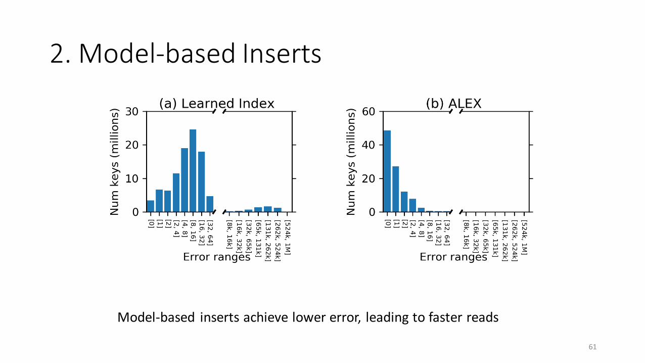
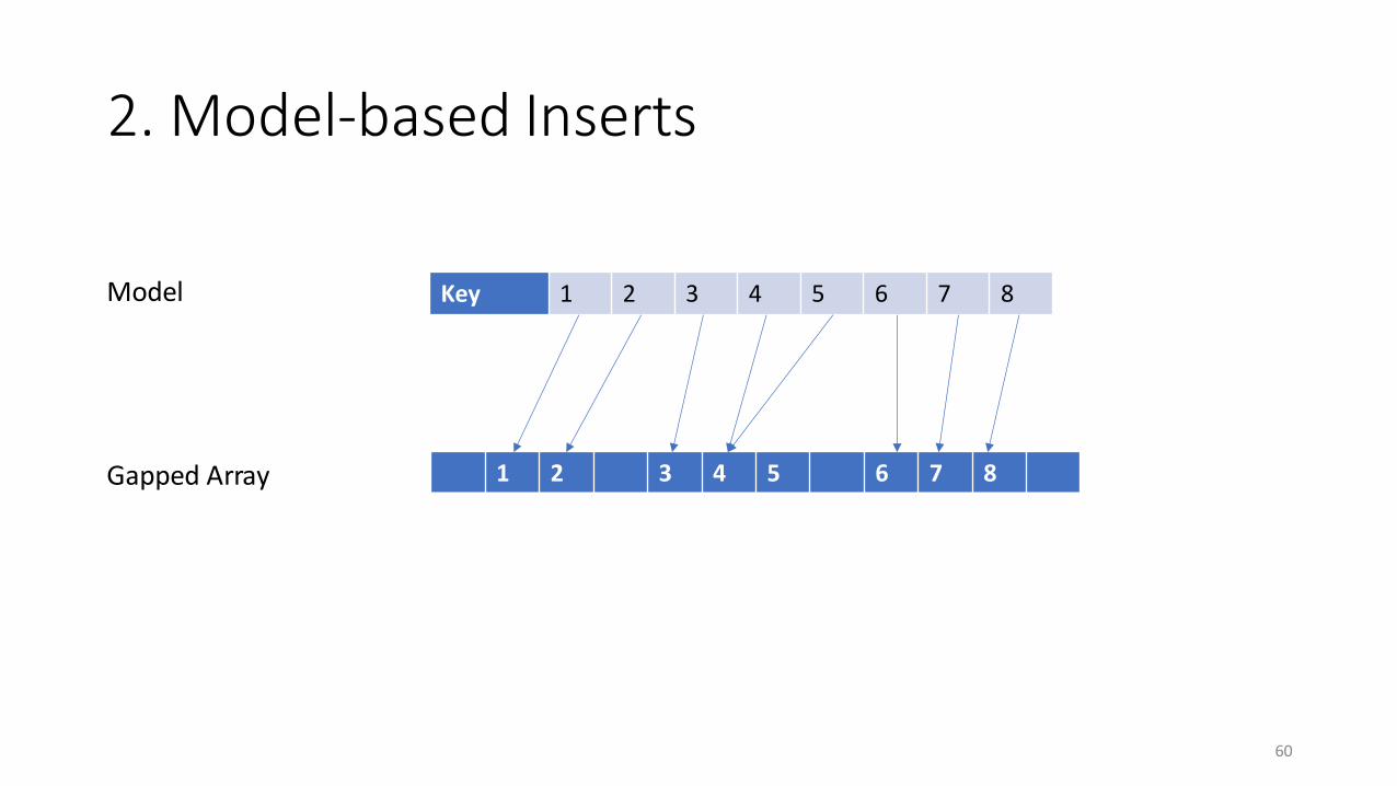
2. Model-based Inserts
61
Model-based inserts achieve lower error, leading to faster reads

3. Adaptive Structure
• Flexible tree structure• Split nodes sideways
• Split nodes downwards
• Expand nodes
• Merge nodes, contract node
• All decisions are made to maximize performance• Uses a cost model of query runtime
62
Learned Data Structures
• A lot more work on different data structures• Multi-dimensional indexes
• Hash Tables
• Bloom Filters
• Suffix Trees
• Different models to learn CDFs

Study Break
• How to extend the CDF idea to algorithms like sorting?
• Can you frame sorting as a prediction task?

Sorting

Sorting
• Puts elements of a list in a certain order.

Sorting
• Puts elements of a list in a certain order.
• Numerical order9 1 17 18 3 0 1 4
0 1 1 3 4 9 17 18
A =
Sort(A) =
Sorting
• Puts elements of a list in a certain order.
• Numerical order
• Lexicographic order
9 1 17 18 3 0 1 4
0 1 1 3 4 9 17 18
A =
Sort(A) =
uvw aaa bbc efg gjl abc cba ghe
aaa abc bbc cba efg ghe gjl uvw
A =
Sort(A) =

Sorting
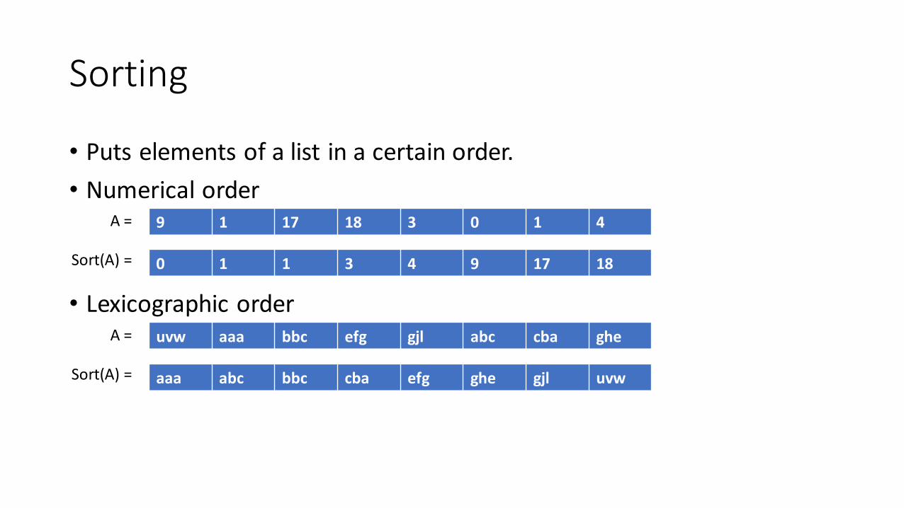
• Puts elements of a list in a certain order.
• Numerical order
• Lexicographic order
• Complex data types such as multi-dimensional, categorical etc have their own specific sort order.
9 1 17 18 3 0 1 4
0 1 1 3 4 9 17 18
A =
Sort(A) =
uvw aaa bbc efg gjl abc cba ghe
aaa abc bbc cba efg ghe gjl uvw
A =
Sort(A) =

Comparison based sorting algorithms

Comparison based Sorting
• Use a comparison function that determines which of two elements should occur first in the final sorted list.
• Compare two elements and then swap if needed.
• Some popular sorting functions: Quick Sort, Heap Sort, Insertion Sort, Tim Sort, Bubble Sort, Selection Sort

Bubble Sort
1. Compare each pair of adjacent elements
2. Swap the two of necessary
3. Repeat Until array is sorted

Bubble Sort Example

Insertion Sort
• Just like sorting a deck of cards.
1. Maintain a sorted deck of cards seen until now.
2. For a new card, find the position in the sorted deck
3. Place the card in the position by shifting the following cards
4. Repeat Until no new incoming card

Insertion Sort Example
Quite fast if numbers are close to actual positions (nearly sorted array )!!
Complexity of comparison-based algorithms
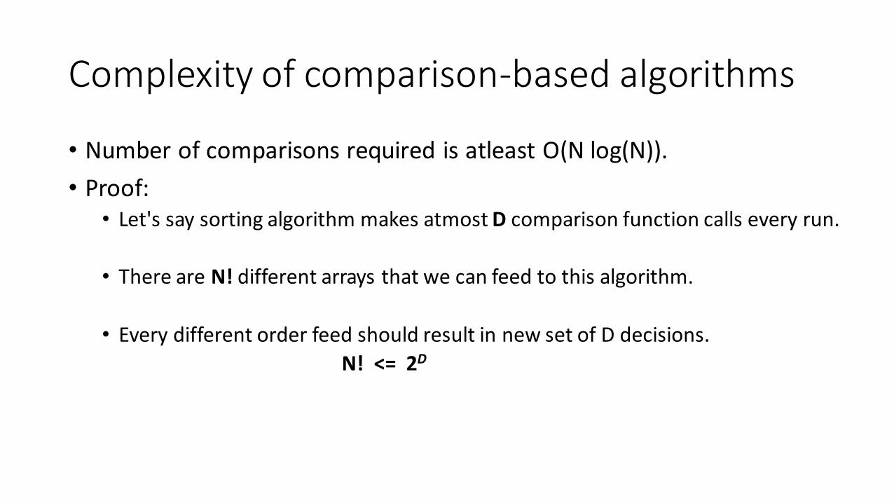
• Number of comparisons required is atleast O(N log(N)).
• Proof:• Let's say sorting algorithm makes atmost D comparison function calls every run.
• There are N! different arrays that we can feed to this algorithm.
• Every different order feed should result in new set of D decisions.
N! <= 2D

Complexity of comparison-based algorithms
• The number of comparisons required is proportional to O(N log(N)).
• Proof:• Lets say sorting algorithm makes atmost D comparison function calls every run.
• There are N! different arrays that we can feed to this algorithm.
• Every different order feed should result in new set of D decisions.
N! <= 2D
Is Nlog(N) the best we can do?

Question
• Given a 1 million sized integer array, if you knew the integers are between 1-100, how would you sort the array?
78

Question
• Given a 1 million sized integer array, if you knew the integers are between 1-100, how would you sort the array?
• Use a 100 sized array to count occurences of each value
79

Distribution based sorting algorithms

Distribution based algorithms
• General idea of distribution-based sorting algorithms:
"Build a histogram of the data and place the data using it"
• Easy to build a histogram if range of the data is limited
Counting Sort
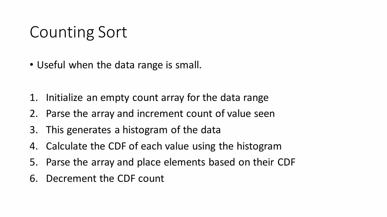
• Useful when the data range is small.
1. Initialize an empty count array for the data range
2. Parse the array and increment count of value seen
3. This generates a histogram of the data
4. Calculate the CDF of each value using the histogram
5. Parse the array and place elements based on their CDF
6. Decrement the CDF count
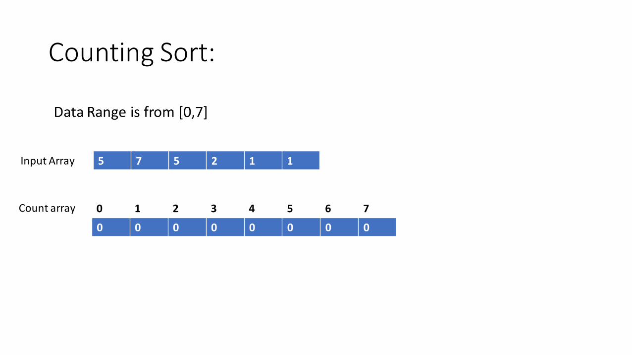
Counting Sort:
Data Range is from [0,7]
5 7 5 2 1 1
0 1 2 3 4 5 6 7
Input Array
Count array
0 0 0 0 0 0 0 0

Counting Sort:
Data Range is from [0,7]
5 7 5 2 1 1
0 1 2 3 4 5 6 7
Input Array
Count array
0 2 1 0 0 2 0 1
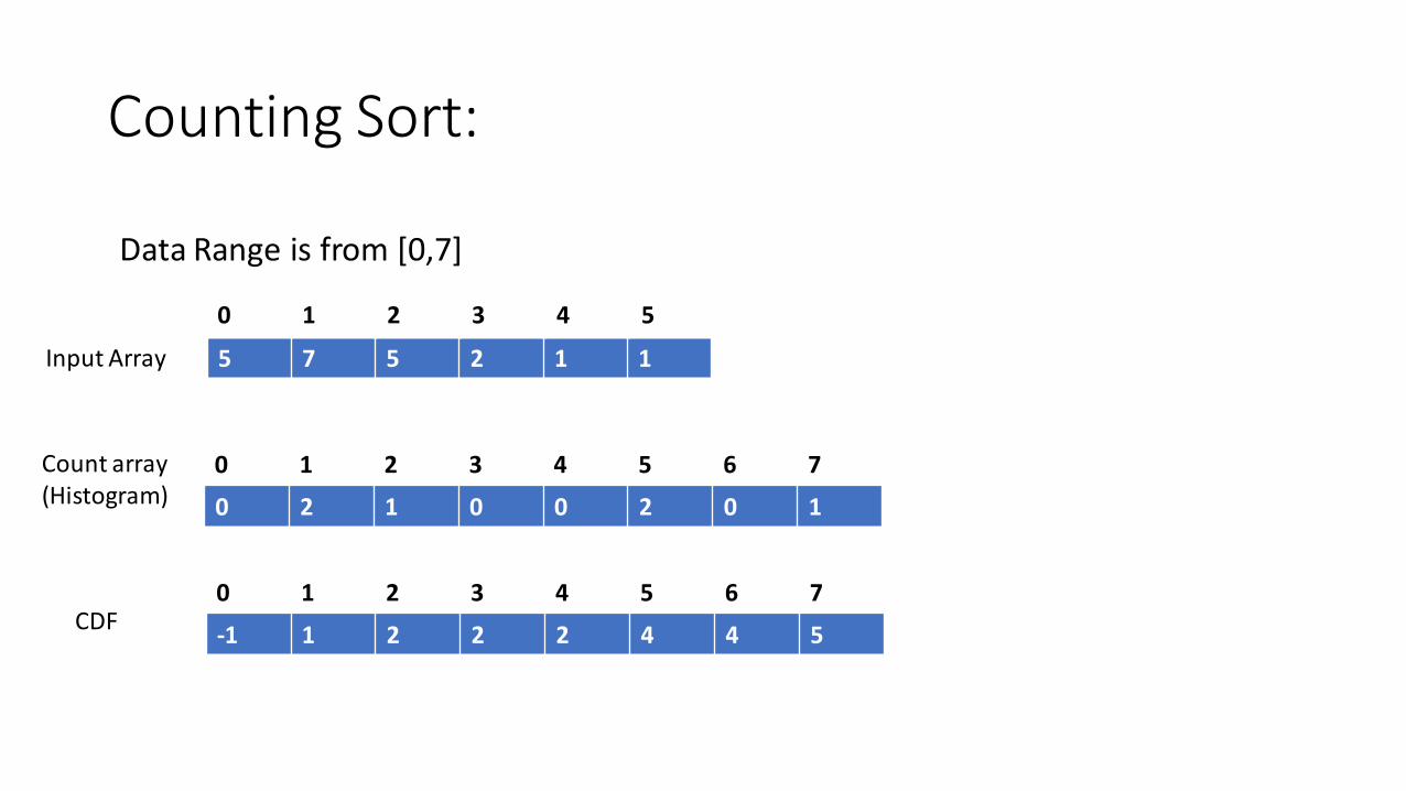
Counting Sort:
Data Range is from [0,7]
5 7 5 2 1 1
0 1 2 3 4 5 6 7
Input Array
Count array(Histogram) 0 2 1 0 0 2 0 1
0 1 2 3 4 5 6 7
-1 1 2 2 2 4 4 5CDF
0 1 2 3 4 5

Counting Sort:
Data Range is from [0,7]
5 7 5 2 1 1
0 1 2 3 4 5 6 7
Input Array
Count array(Histogram) 0 2 1 0 0 2 0 1
0 1 2 3 4 5 6 7
-1 1 2 2 2 4 4 5CDF
0 1 2 3 4 5
1 1 2 5 5 7Output Array

Counting Sort
• Only works if data range small
87

Counting Sort
• Only works if data range small
• How to generalize counting sort?
88

Counting Sort
• Only works if data range small
• How to generalize counting sort?
89
Operate on small segments of data

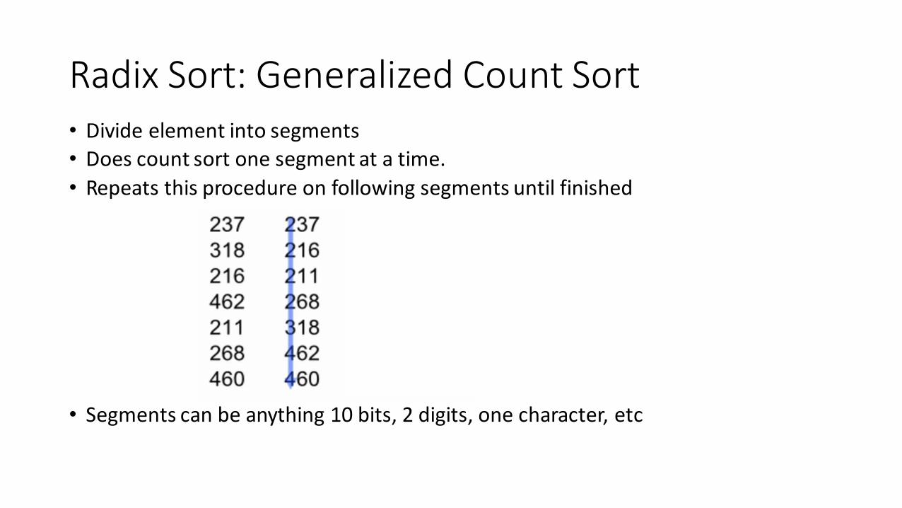
Radix Sort: Generalized Count Sort• Divide element into segments
• Does count sort one segment at a time.
• Repeats this procedure on following segments until finished
• Segments can be anything 10 bits, 2 digits, one character, etc
Radix Sort: Generalized Count Sort• Divide element into segments
• Does count sort one segment at a time.
• Repeats this procedure on following segments until finished
• Segments can be anything 10 bits, 2 digits, one character, etc

Radix Sort: Generalized Count Sort• Divide element into segments
• Does count sort one segment at a time.
• Repeats this procedure on following segments until finished
• Segments can be anything 10 bits, 2 digits, one character, etc
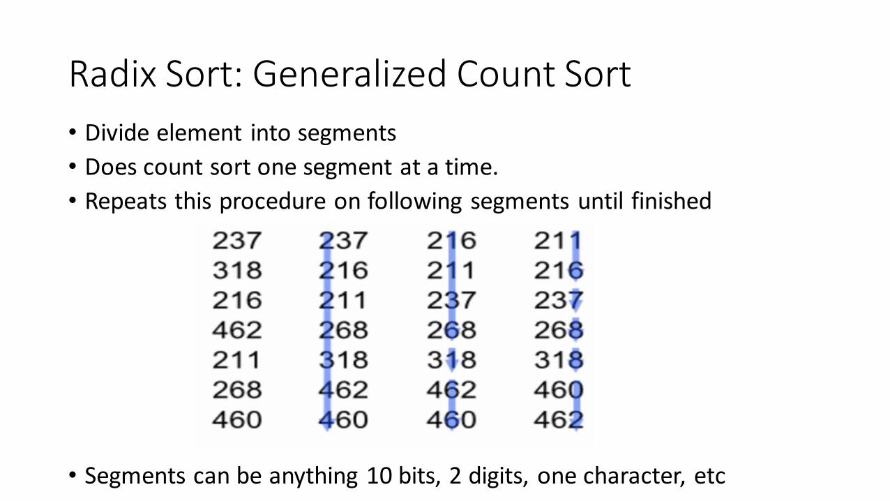
Radix Sort: Generalized Count Sort
• Divide element into segments
• Does count sort one segment at a time.
• Repeats this procedure on following segments until finished
• Segments can be anything 10 bits, 2 digits, one character, etc

Distribution based algorithms complexity
• Assuming the data elements have atmost W digits, the complexity of radix sort is atmost O(NW).
• This might be better than NLogN based on W
• Generally, for numerical data 32, 64, 128 bit integers radix sort is much faster than comparison-based sorts.

Distribution based algorithms
• Essentially generate CDF of the data by counting
Can we use ML models to model CDF?

A Learned Sorting Algorithm

Sorting as a prediction task
• Sorting is essentially a prediction task
• Sorting involves predicting the correct final position of the element based on its value
• The algorithms indirectly calculate the position of the element using some operations and place it there
• We can potentially use models for doing this instead of algorithms.
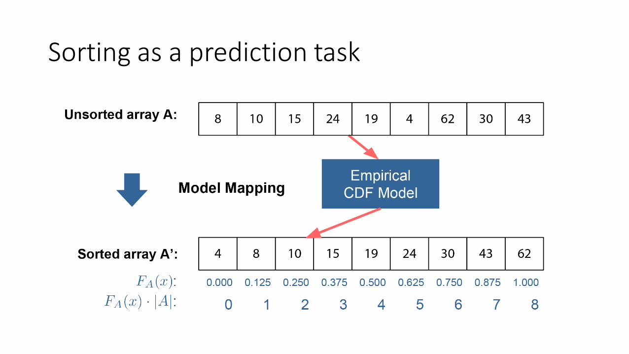
Sorting as a prediction task
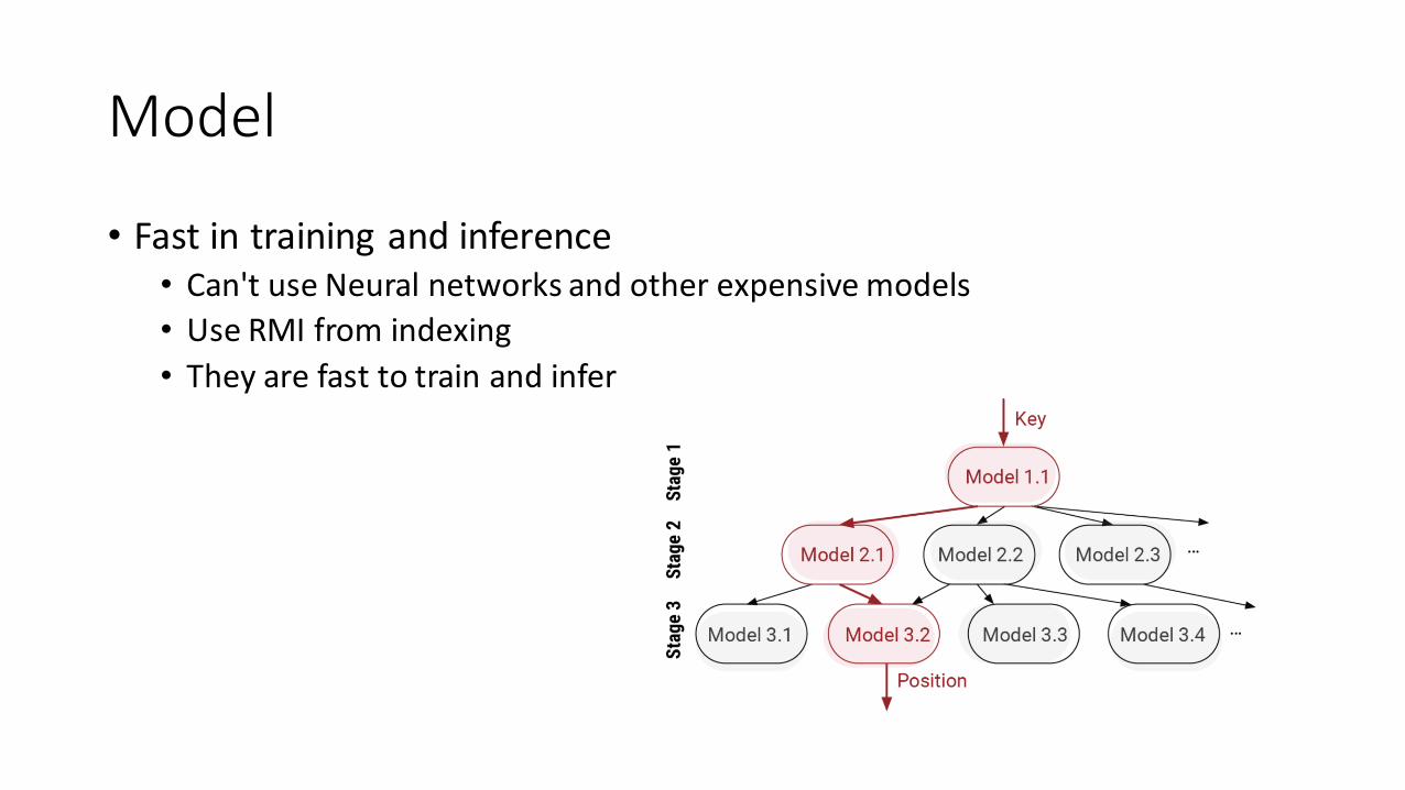
Model
• Fast in training and inference• Can't use Neural networks and other expensive models
• Use RMI from indexing
• They are fast to train and infer
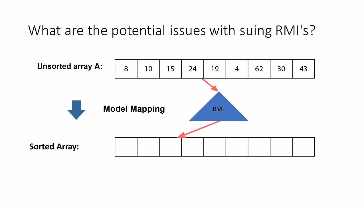
What are the potential issues with suing RMI's?
RMI
InSorted Array: 1515 10

Sorting with RMIs
RMI
InNearly Sorted Array:
43
24
19
1515 10

Issues with directly using model
• Collisions: two elements get mapped to the same place
• Imperfect mapping: array may not be monotonic

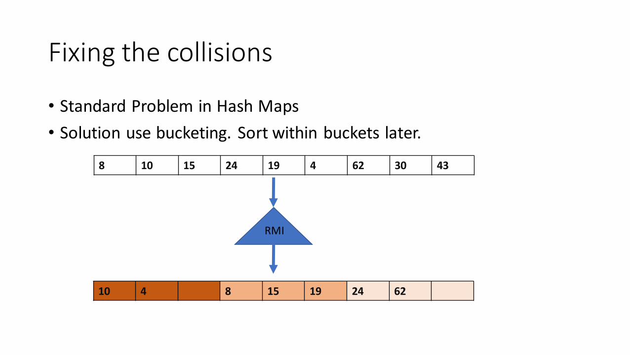
Fixing the collisions
• Standard Problem in Hash Maps
• Solution use bucketing. Sort within buckets later.
8 10 15 24 19 4 62 30 43
8
RMI

Fixing the collisions
• Standard Problem in Hash Maps
• Solution use bucketing. Sort within buckets later.
8 10 15 24 19 4 62 30 43
10 8
RMI

Fixing the collisions
• Standard Problem in Hash Maps
• Solution use bucketing. Sort within buckets later.
8 10 15 24 19 4 62 30 43
10 8 15
RMI

Fixing the collisions
• Standard Problem in Hash Maps
• Solution use bucketing. Sort within buckets later.
8 10 15 24 19 4 62 30 43
10 8 15 24
RMI

Fixing the collisions
• Standard Problem in Hash Maps
• Solution use bucketing. Sort within buckets later.
8 10 15 24 19 4 62 30 43
10 8 15 19 24
RMI

Fixing the collisions
• Standard Problem in Hash Maps
• Solution use bucketing. Below bucket Size=3
8 10 15 24 19 4 62 30 43
10 4 8 15 19 24
RMI

Fixing the collisions
• Standard Problem in Hash Maps
• Solution use bucketing. Sort within buckets later.
8 10 15 24 19 4 62 30 43
10 4 8 15 19 24
RMI
Fixing the collisions
• Standard Problem in Hash Maps
• Solution use bucketing. Sort within buckets later.
8 10 15 24 19 4 62 30 43
10 4 8 15 19 24 62
RMI

Fixing the collisions
• Standard Problem in Hash Maps
• Solution use bucketing. Sort within buckets later.
8 10 15 24 19 4 62 30 43
10 4 8 15 19 24 62 30
RMI

Fixing the collisions
• Standard Problem in Hash Maps
• Solution use bucketing. Sort within buckets later.
8 10 15 24 19 4 62 30 43
10 4 8 15 19 24 62 30
RMI
43
Bucketing Reduces Collisions!! But does not eliminate them!!

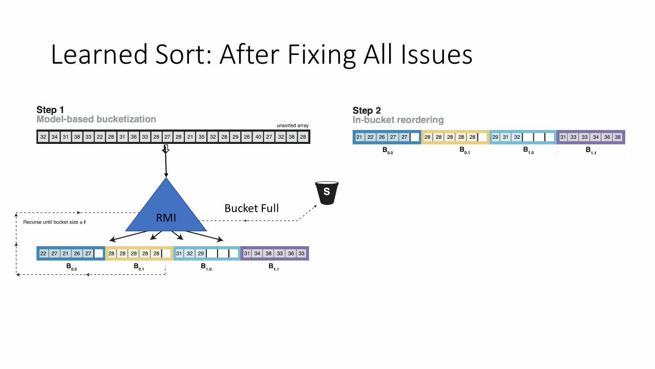
Fixing the collisions: monotonicity not garantued• Standard Problem in Hash Maps
• Solution use bucketing. Sort within buckets later.
• When bucket full, throw the extra bucketin a separate array.
8 10 15 24 19 4 62 30 43
10 4 8 15 19 24 62 30
RMI
43
Bucketing Reduces Collisions!! But does not eliminate them!!

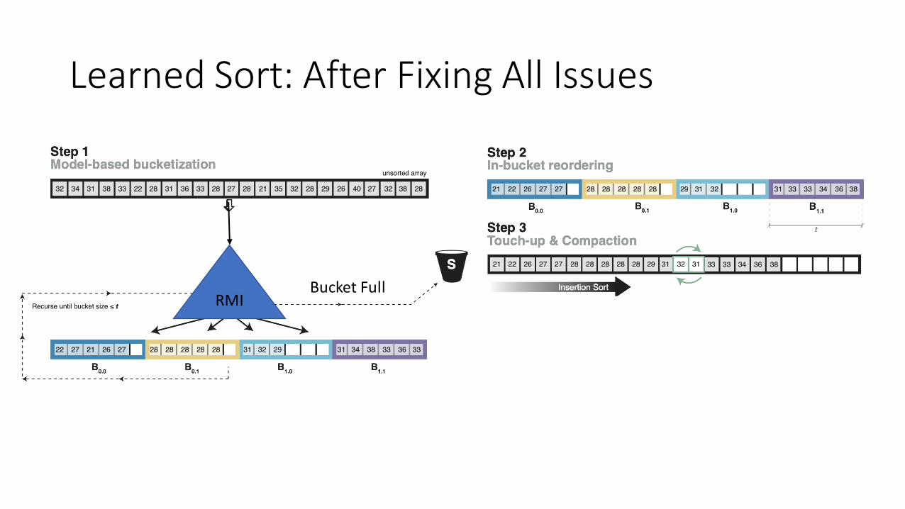
Imperfect Array
• Since the array is nearly sorted.
• We use a fast-sorting algorithm for nearly sorted array.
• Insertion Sort is good for such cases.

Learned Sort: After Fixing All Issues
RMIBucket Full
Learned Sort: After Fixing All Issues
RMIBucket Full
Learned Sort: After Fixing All Issues
RMIBucket Full

Learned Sort: After Fixing All Issues
RMIBucket Full

Performance of Learned Sort
• How do you expect it to perform w.r.t Radix Sort
Performance of Learned Sort
• How do you expect it to perform w.r.t Radix Sort
• It is much Slower than Radix Sort!!
• But why is it slow?

Random access by the model
121

Performance of Learned Sort
• How do you expect it to perform w.r.t Radix Sort
• It is much Slower than Radix Sort!!
• Model does a lot of random accesses while mapping elements in buckets
• Solution: Use small number buckets(~1000) so they fit in cache. Then recursively divide bucket into smaller buckets.

Recursive Partition: fanout=2
8 10 15 24 19 4 62 30 438 keys

Recursive Partition: fanout=2
8 10 15 24 19 4 62 30 438 keys
2 buckets x 4 8 10 15 4 24 19 62 30

Recursive Partition: fanout=2
8 10 15 24 19 4 62 30 438 keys
2 buckets x 4 8 10 15 4 24 19 62 30
4 buckets x 2 8 4 10 15 24 19 62 30
Learn Sort Fanout depends on L2 cache size!! (Around 1k-5k)

Multi layered Learned Sort algorithm

Cache Efficeint Learned Sort
• How would this perform compared to Radix Sort?
127

Radix Sort vs Learned Sort:
• Learned Sort is 1.5x faster than Radix Sort on 64 bit integers
• Reason: Learned Sort does fewer number of passes over the data

Summary
• Performance of data structures and algorithms can be enhanced by learned models of data and query distribution
• ML models cannot be simply plugged in
• ML enhanced data structures and algorithms require careful design
• Need to consider Models + Systems + Algortihms
129