Learning Continuous Probability Distributions with

COGNITIVE SCIENCE 17, 463-496 (1993)

Learning Continuous Probability Distributions with Symmetric Diffusion Networks

JAVIERR.MOVELLAN University of California, San Diego

JAMES L.MCCLELLAND Carnegie Mellon University

in this article we present symmetric diffusion networks, a family of networks that instantiate the principles of continuous, stochastic, adaptive and interactive propagation of information. Using methods of Markovlon diffusion theory, we for-

malize the activation dynamics of these networks and then show that they can be trained to reproduce entire muitivariote probability distributions an their outputs using the contrastive Hebbian learning rule (CHL).,We show that CHL performs

gradient descent on an error function that captures differences between desired and obtolned continuous multivoriate probability distributions. This allows the

learning algorithm to go beyond expected values of output units and to approximate complete probability distributions on continuous muitivariote activation spaces. We argue that learning continuous distributions is an important task

underlying a variety of real-life situations that were beyond the scope of previous connectionist networks. Deterministic networks, like back propagation, cannot ieorn this task because they ore limited to learning average values of indepen-

dent output units. Previous stochastic connectionist networks could learn pro- bobility distributions but they were limited to discrete variables. Simulations show that symmetric diffusion networks can be trained with the CHL rule to op- proximate discrete and continuous probability distributions of various types.

1. INTRODUCTION

Learning can be seen as the process of detecting and storing how some events (inputs) affect the behavior of other events (outputs). If the inputs have no effect on the outputs they are statistically independent, otherwise there is a contingency. Contingencies can be seen as a class of functions mapping the space of inputs onto the space of possible.probability distributions of the outputs. Contingencies may occur when the inputs have an

The preparation of this article was supported by NIMH Career Development Award MNOO385, NSF Grant BNS 88-12048, and by NIMH grant MH47566. The computational resources used were supported by NSF grant DIR 91-02196.

We would like to thank Paul Smolensky and Brian MacWhinney for many useful com- ments on an earlier draft of this article.

Correspondence and requests for reprints should be sent to Javier R. Movellan; Depart- ment of Cognitive Science, University of California Q San Diego, La Jolla, CA 92093-0515.

463

464 MOVELLAN AND MCCLELLAND

effect on the average value of individual output variables. For example, economic policies may have an effect on the average income or the average level of education of a country. There may also be contingencies that affect other aspects of the output’s behavior such as the shape of the probability distribution of the outputs or the way these outputs correlate with each other. For example, different economic policies may affect the distribution of wealth or the correlation between wealth and education without affecting the average income. Such examples come up all the time in cognitive and perceptual domains. The Necker cube is perhaps the most famous case. The perception of the individual elements of the cube-each vertex, for example, or each line-is certainly contingent on the stimulus, but in a very dis- tinctive and particular way. Two quite different interpretations of each vertex are possible, and these are not well characterized by their average value. Furthermore, the probability that we will see one vertex as being on the front face of the cube is strongly dependent on how we see each of the other vertices. With the necker cube there are in fact two very probable whole percepts-full sets of interpretations of the vertices-and many other much less likely ones. Whereas the Necker cube is, of course, an artifact, many natural stimuli-shadows, for example, or ambiguous words or sen- tences-often support a distribution of interpretations that is very poorly characterized by the central tendency of individual elements. It is, therefore, desirable to develop learning algorithms capable of learning contingencies that go beyond effects on average values. Connectionist learning algorithms have proven to be useful contingency detectors but most can only be applied in situations where the goal is to learn only the expected values of the outputs.

For example, back propagation networks (Bryson & Ho, 1969; Le Cun, 1985; Parker, 1985; Rumelhart, Hinton, & Williams, 1986; Werbos, 1974) are functions defined from the space of possible inputs to the space of possible outputs. They are typically trained with a learning rule that minimizes the total sum of squared errors (TSS) between desired and obtained outputs. It is easy to show that among all possible functions from the space of inputs to the space of outputs there is one that achieves minimum TSS. This function, which is called the regression function, assigns to each input vector the average of the training outputs conditional on that input (Papoulis, 1990). Back-propagation learning and other forms of nonlinear regression can be seen as methods for estimating regression functions. This is precisely what is needed with a particular type of contingency, which we refer to as “signal + noise” contingencies. In this type of contingency, the underlying association between input and output (the signal) is deterministic but per- turbed by the effects of an additive independent random variable (the noise). The signal is the expected value of the output for each of the inputs, and can be estimated by averaging samples of training outputs that share the same inputs. This tendency to average samples of outputs with common

CONTINUOUS PROBABILITY DISTRIBUTIONS 465

inputs is shared by all regression methods but it is not appropriate in all cases. This is particularly clear in situations where there is more than one correct output for each input but the average of these outputs is not a correct solution.

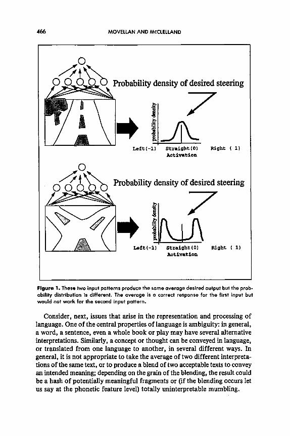
Consider for instance the vehicle navigation problem displayed on Figure 1. A back-propagation (BP) network is presented with road images as input and with appropriate steering directions as desired output. In the example the steering direction is represented by the activation of an output unit. Positive and negative values represent the degree of right and left steering. Figure 1 displays a case where two input images have an effect on the shape, but not the average value, of the distribution of desired actions. With this particular configuration back propagation learns the same output for the two road images, clearly an undesirable solution.’

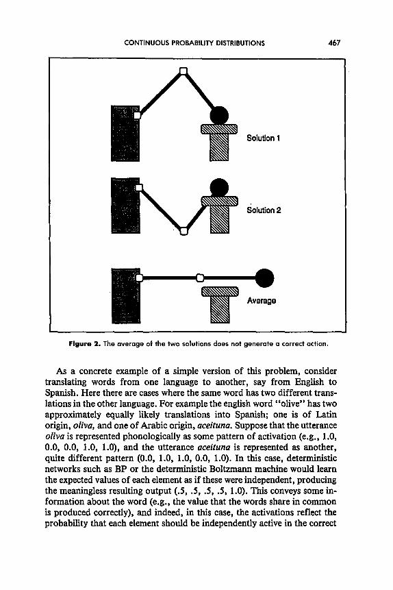
A similar situation arises in motor control when one has to choose a combination of joint angles to reach desired locations. One approach is to train a network with samples of “action- outcome” pairs and then use the trained network to select appropriate actions when desired outputs are specified. This method is known as direct-inverse modeling. Jordan and Rumelhart (1992) discussed a difficulty faced with this approach. In many cases, the mapping from actions to outcomes is many-to-one, so that the mapping from outcomes to actions is one-to-many. Most problematic are cases in which the set of acceptable actions forms a nonconvex region in action space (Jordan & Rumelhart, 1992). Figure 2 shows one such case in which two different settings of joint angles in a robot arm place the arm at the same goal location but the average of these two settings places the arm in quite a different place. When a deterministic network such as BP is used to learn such a mapping, it finds an average; the difficulty is that the average need not fall within the set of possible solutions, as the figure makes clear.

There are two problematic features to the averaging problem. One is that it computes an average value for each unit, thereby losing information about the actual range or distribution of allowed values. The other, deeper problem, is that it looses information about dependencies among the different dimensions of the output. In the robot arm example, we do not in general get a satisfactory result if we merely choose one of the acceptable values for each of the two joint angles independently; rather, what counts as an acceptable reach for the object is a particular combination of joint angles. Such combinations can be viewed as regions in a multidimensional space. If we can choose such combinations in a way that matches a probability distribution that is nonzero only in those regions of the space that correspond to acceptable actions, we will have learned to solve the problem.

’ The purpose of this example is to illustrate the need of going beyond expected values. Dean Pomerleau’s (1991) ALVINN system encountered a problem similar to the one mentioned here, but he solved it using another approach.


obability density of desired steering

Left{-1) Straight(O) Right ( 1)

Probability density of desired steering

* *I($

Leftz(-1) Straight(O) Right ( 1) hotivation

Figure 1. These two input patterns produce the same average desired output but the probability distribution is different. The average is a correct response for the first input but would not work for the second input pattern.

Consider, next, issues that arise in the representation and processing of language. One of the central properties of language is ambiguity: in general, a word, a sentence, even a whole book or play may have several alternative interpretations. Similarly, a concept or thought can be conveyed in language, or translated from one language to another, in several different ways. In general, it is not appropriate to take the average of two different interpretations of the same text, or to produce a blend of two acceptable texts to convey an intended meaning; depending on the grain of the blending, the result could be a hash of potentially meaningful fragments or (if the blending occurs let us say at the phonetic feature level) totally uninterpretable mumbling.


Solution 1

Solution 2

Figure 2. The average of the two solutions does not generote a correct action.

As a concrete example of a simple version of this problem, consider translating words from one language to another, say from English to Spanish. Here there are cases where the same word has two different translations in the other language. For example the english word “olive” has two approximately equally likely translations into Spanish; one is of Latin origin, olivu, and one of Arabic origin, aceituna. Suppose that the utterance ofiva is represented phonologically as some pattern of activation (e.g., 1 .O, 0.0, 0.0, 1.0, l.O), and the utterance uceituna is represented as another, quite different pattern (0.0, 1 .O, 1 .O, 0.0, 1 .O). In this case, deterministic networks such as BP or the deterministic Boltzrnann machine would learn the expected values of each element as if these were independent, producing the meaningless resulting output (.5, .5, .5, .5, 1.0). This conveys some information about the word (e.g., the value that the words share in common is produced correctly), and indeed, in this case, the activations reflect the probability that each element should be independently active in the correct


response. But it does not convey enough information to specify which combinations of features must be on or off to produce one or the other of the possible correct alternatives.

In this article we explore the use of stochastic networks to solve the types of problems described previously. In doing so, we hope to help to con- solidate a way of thinking about stochastic networks that has not received as much explicit treatment as it deserves. This is the idea that stochastic networks should be viewed as computing functions of their inputs, just like deterministic networks. In this case, the function is not from inputs to expected values of outputs, but from inputs to entire probability distributions of outputs. This idea is certainly an important part of the stochastic network theory introduced by Geman and Geman (1984), Ackley, Hinton, and Sejnowski (1985), and was particularly emphasized by Smolensky (1986). But in the main, stochastic networks have been used in neural network research as procedures for finding the single best pattern, through the process of simulated annealing, and not for actually modeling distributions of desired states.

Once we see stochastic networks as mappings from inputs to multivariate probability distributions, we can treat learning as a matter of modifying connection weights between units to make the obtained and desired probability distributions as similar as possible. In this article we use this approach with a class of networks that we will call “symmetric diffusion networks” (SDN). SDN’s are one instantiation of the principles of continuous, stochastic, adaptive, and interactive human information processing proposed by McClelland (in press) on the basis of earlier computational and psychological research. These principles were put together to provide a general framework for modeling normal and disordered cognition. SDNs are collec- tions for processing units organized in modules with symmetric bidirectional connections. Each unit collects a net input from all the units to which it is connected and generates a real valued, bounded activation. These activation values are continuous random variables with a probability density controlled by the net input.

Using Markovian diffusion theory (Gillespie, 1992) we derive the equilibrium distribution of SDNs and show that the contrastive Hebbian learning rule (CHL) can be used to learn entire probability distributions. CHL is a general learning rule previously applied to a variety of models including the discrete Hopfield model (Hopfield, Feinstein, 8c Palmer, 1983), the original stochastic Boltzmann machine (Ackley et al., 1985), the harmonimum (Smolensky, 1986), the deterministic Boltzmarm machine (Galland & Hinton, 1989; Hinton, 1989; Peterson & Anderson, 1987), and the continuous Hopfield model (Movellan, 1990). Here we show that in SDNs, the CHL rule performs gradient descent on an error function that captures differences between entire distributions.


There are many important precursors to this work. Ratcliff (1978) used a simple diffusion process to model memory retrieval. The use of Gaussian noise in continuous Hopfield networks was independently explored in Akiyama, Yamashita, Kajiura, & Aiso (1989) in work on Gaussian machines. This work was focused in optimization problems and no learning algorithm or formal desciption of the network behavior was proposed. The importance of learning probability distributions was pointed out by Smolensky (1986) and certainly many of the ideas in this article are related to the seminal work in harmony theory (Smolensky, 1986), and the original stochastic Boltzmann machine (SBM). In a previous article (Movellan and McClelland, in press), we presented initial work with the CHL algorithm and another instantiation of the principles of continuous, stochastic, interactive processing. Our approach there was based on the ideas of contrastive learning (Baldi & Pineda, 1991; Movellan, 1990) rather than Markovian diffusion theory. It should be noted that SBM can learn discrete binary probability distributions. However to our knowledge, this aspect of the SBM has hardly ever been explored. The SBM has generally been used to learn deterministic mappings, where it is typically less efficient than deterministic networks such as BP or deterministic Boltzmann machines (DBMS). Our work can be seen in part as an investigation of this relatively neglected property of SBMs. We also extend the previous work by formalizing the behavior of continuous stochastic networks and showing how they can be trained to learn continuous as well as discrete probability distributions.

What follows is a formal presentation of SDNs and a derivation of the CHL rule for learning probability distributions with these networks. We also present simulations showing that SNDs can indeed be trained to approximate discrete and continuous probability distributions of various types.

2. ACTIVATION DYNAMICS

From a mathematical point of view, SDNs ar Markovian diffusion processes governed by a system of stochastic differential equations. These equations consist of a drift term and a diffusion terms. The drift is the deterministic kernel of the process controlling the instantaneous average velocity of the activation vector. The diffusion term controls the instantaneous variance of the activations. SDNs may be instantiated in a variety of ways. The specific instantiation that we use in this article has a drift controlled by a variation of the continuous Hopfield (1984) model. The diffusion in this instantiation is a constant, u, which controls the level of noise in the network.

More specifically, let a = [al,. . . , a,Jr be a real-valued activation column vector. Let W = [wl, . . . , w,,] be a real valued symmetric matrix of connections, where each wi = [wr,i,. . . , wn,i]r is the fan-in column vector of


connections to the unit i. The evolution of the activations is governed by the following system of stochastic differential equations:

dai = (neti - niti)dt+ OdiZi(t);i= l,...,n (1)

where Z/(t) is a standard independent Gaussian random variable; neti = aTwi; ni% = 1 / gif(ai); gi is a gain term that scales the response of f(x); f(x) is the inverse of a bounded continuous monotonic activation function f - I; the j(x) function maps the bounded real-valued activation space (min,max) c 3, into the entire real line (e.g., the logit or the probit functions). In our simulations we use a scaled version of the logit function, also known as the inverse logistic

Ui - min ngti = ;flUi) = + log may - Ui. (2)

where max and min bound the activation range. A precise treatment of Equa- tion 1 can be given in reference to Ito’s stochastic calculus (Gardiner, 1985) but for the purpose of this article it is sufficient to view it as determining the limiting solution of a difference equation where the At is made infinitesimally small. The term n&i = 1 / gif(ai) represents the net input required to main- tain an activation value of ai. If the actual net input, neti, is smaller than the required net input, kti, the activation decreases; if bigger, it increases. The second term in the equation adds up Gaussian noise to this process with the amount of noise being controlled by the parameter u.

Equation 1 is known as a Langevin description of a Markovian diffusion process with a drift vector

driFt(a) = net(a) - &(a) (3)

and a diffusion matrix given by aI, where I is the unit matrix. It is easy to show (Hopfield, 1984) that when the weight matrix is sym-

metric, the drift vector is the exact gradient of a Hopfield style goodness function of the following form

G(a) = H(a) - S(a) (4)

where

H(a) = +aTWa (5)

is the harmony or consistency between the network activations and the weight constraints. The stress


is the weighted sum of penalty terms, si, for the activations departing from rest value

where rest = f(O). In our implementation, the stress is given by the following equation

Si = (Ui - min)lOg(Ui - min) + (mc7X - Ui)lOg(mUX - c7i) (8)

max - min 2

lOg may ; min _ max ; min ,Og max ; min

The goodness of a particular activation vector is commonly interpreted as the degree of consistency of this vector with the knowledge captured in the network’s weights and gain. The harmony term, H, captures the degree of match with the expected correlations between pairs of units. This knowledge is embedded in the weights: Units connected with positive weights are more “harmonious” if they have activations of the same sign, and units with negative weights are more “harmonious” when their activations have opposite signs. The stress term, S, captures how extreme the activations are expected to be. When the gain terms, gi, are large, extreme activation values are expected.

Since the drift is the exact gradient of the goodness function

drift(a) = VG(a) = nit(a) - net(a) (9)

then - G(a) can be seen as a potential field and the drift as the force field generated by that potential. When the diffusion term vanishes, the network becomes deterministic and goodness can only increase through time. Since the goodness function is bounded upward, the activations stabilize at local maxima of G. It is also known that this deterministic kernel (when (z = 0) is trainable with the CHL rule, but that instabilities may occur due to the existence of multiple maxima in the G function (Hinton, 1989; Movellan, 1990; Peterson & Anderson, 1987; Peterson & Hartman, 1989).

2.1 The Diffusion of Probability The stochastic nature of SDNs encourages a revision of the language used to describe the behavior of the network. Because the network is not deterministic, the trajectory of the activations can no longer be predicted from initial states. What we can say is that, most of the time, the network activations will be in certain regions, less of the time in other regions, and so on. Thus, we need to describe the network in terms of probability distributions and its dynamics in terms of changes in probability distributions throughout time.


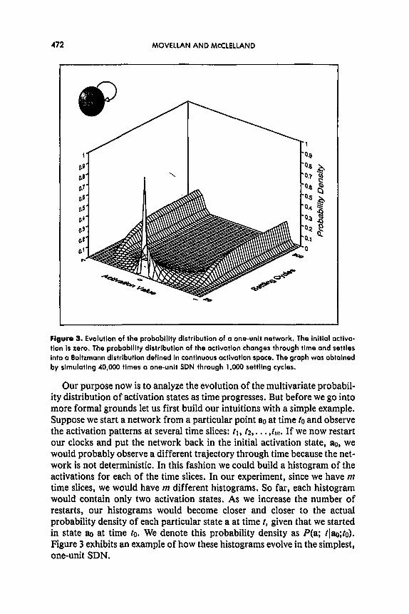
Figure 9. Evolution of the probability distrlbutlon of a one-unit network. The initial actlva-

tion Is zero. The probability distribution of the octlvation changes through tlme and settles into a Boltzmann dlstrlbutlon defined In continuous activation space. The graph was obtained by simulating 40,000 times a one-unlt SDN through 1,000 settling cycles.

Our purpose now is to analyze the evolution of the multivariate probability distribution of activation states as time progresses. But before we go into more formal grounds let us first build our intuitions with a simple example. Suppose we start a network from a particular point a0 at time fo and observe the activation patterns at several time slices: tr, t2,. . . J,,,. If we now restart our clocks and put the network back in the initial activation state, ao, we would probably observe a different trajectory through time because the network is not deterministic. In this fashion we could build a histogram of the activations for each of the time slices. In our experiment, since we have m time slices, we would have m different histograms. So far, each histogram would contain only two activation states. As we increase the number of restarts, our histograms would become closer and closer to the actual probability density of each particular state a at time r, given that we started in state a0 at time to. We denote this probability density as P(a; tlac;tc). Figure 3 exhibits an example of how these histograms evolve in the simplest, one-unit SDN.


Let us try to understand this evolution from yet another point of view. We can think of probability density as an abstract “substance” that propa- gates through the different states of the network according to some simple diffusion principles. We may think of a restart in a particular state, a~, as a concentration of all the available probability in that one state. Probability then flows or diffuses to other states according to Equation 1, which reflects two opposing principles: (1) local optimization of goodness: move in directions that maximize goodness, a principle embedded in the drift term (n& - n&); and (2) local optimization of entropy, a principle controlled by the diffusion parameter, u. Eventually, we may guess, the probability of the activation states stabilizes into an equilibrium distribution where each state receives as much probability as it sends. In fact, our guesses can be proven to the right. A well-known result in Markovian diffusion theory (Gardiner, 1985) is that processes defined by a Langevin-type stochastic equation satisfy the forward Fokker-Planck diffusion equation. It is also known that this equation models the diffusion of a “substance,” in this case probability, according to the previously mentioned principles. In the SDN case, the Fokker-Planck equation can be shown to assume the following form:

am; +o); to) = at - V * [drift(a) P(a; I.lao; to)] + f v2 P(s; tlag; to). (10)

The Fokker-Planck equation fully describes the temporal evolution of the probability density of the activation states, a, given a starting point, a~. The symbol V - is the divergence operator

V . [drift(a) l’(a; tlm; lo)] = k , p l --& NWa) P(a; h; toI1 (11)

and V’ is the divergence of the gradient, also known as the Laplace operator,

k v P(a; t)ao; 10) = V * V P(a; 4ao; to) = i = 1 aa P(a;;J,ao: to) (12)

The divergence of a vector field has the following standard interpretation: Consider a substance spreading at each point, a, in a multidimensional field with velocity v(a). It can be shown that the negative of the divergence of v(a) represents the inflow of substance per unit volume at that point. Because the first term in the right side of Equation 10 has a negative sign, it tells us that the probability is flowing throughout the entire activation space with a velocity component equal to the drift times the probability. The effect of this term is to spread more probability towards the better states.

The second term in the right side of Equation 10 is the Laplacian of the probability. The Laplacian is the divergence of the gradient and, thus, it tells us that probability is also flowing with a velocity component opposite


to the gradient of the probability. The result of this flow is to move probability from states with more probability towards states with less probability. The relative importance of the first and second terms in the right side of Equation 10 is governed by the u parameter. We will now show that as time progresses, the probability distribution equilibrates at a point where each state receives as much probability as it sends. At that point, the network is said to be at stochastic equilibrium.

2.2 Stochastic Stability We already know that for the deterministic kernel, the activations stabilize in local maxima of the goodness function. In the stochastic case it is clear that activations cannot stabilize because Gaussian noise is constantly injected to the network. However, in the stochastic case we can investigate whether the probability distribution of activation states stabilizes over time and whether these stable distributions depend on the starting conditions. This is an important issue in our present work because we are interested in learning stable distributions over a set of output variables.

To simplify the proof that these networks exhibit stochastic stability, we discretize time and partition the activation space into an arbitrarily large number of hypercubes. SDNs satisfy the conditions of an important theorem in Markov process theory known as the Markovian basic limit theorem (Taylor & Karlim, 1984). SDNs are Markovian because the most recent state provides all available information about future states. They are also regular processes because given enough cycles, there is a nonzero probability of moving from any hypercube to any other hypercube in activation space. Given these two conditions, the Markovian basic limit theorem guar- antees the three following properties: (1) there exists a limiting distribution; (2) the limiting distribution is unique and independent of the starting conditions; and (3) this limiting probability distribution equals the long-run proportion of time that the process will be in each of the hypercubes.

The fact that there is a limiting distribution that is unique will, in principle, solve the problem of multistability that we find in deterministic networks. The third property is sometimes referred to as ergodicity. When a network is ergodic, the equilibrium probability distribution can be interpreted in two very different ways: We may use several trials restarting the network from random points and letting it settle for a sufficient criterion time, tC 2 to. The equilibrium probability of a state hypercube can then be estimated by collecting the proportion of trials that the network is in that region at time tC. We may also use a single trial and record the long-run proportion of time spent in that region in this single trial. If the network is ergodic, this second estimate also converges to the equilibrium probability distribution. We will use this property to design efficient methods of collecting equilibrium distribution statistics.


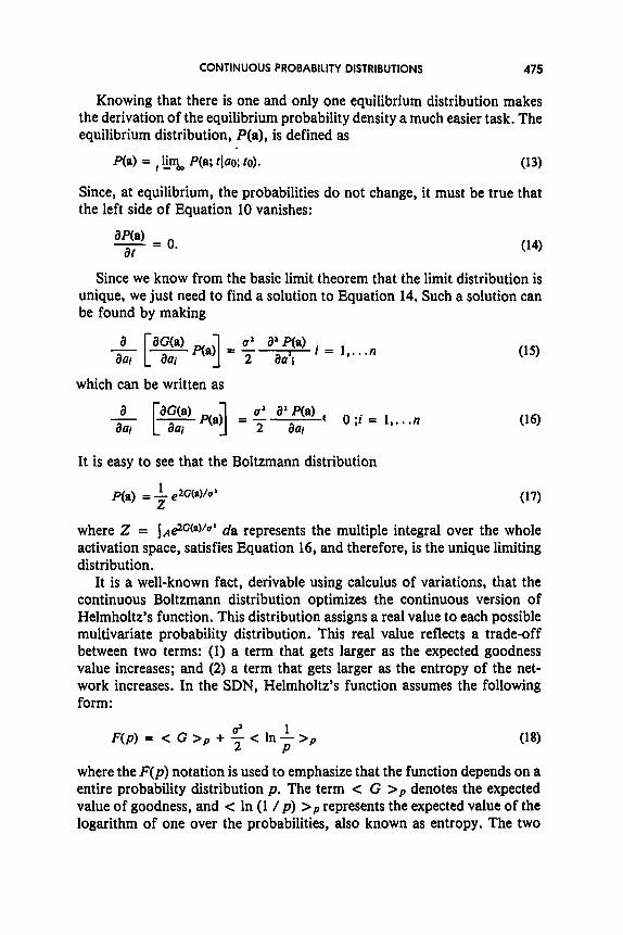
Knowing that there is one and only one equilibrium distribution makes the derivation of the equilibrium probability density a much easier task. The equilibrium distribution, P(a), is defined as

Ha) = , l& P(a; 11~0; to). (13)

Since, at equilibrium, the probabilities do not change, it must be true that the left side of Equation 10 vanishes:

Since we know from the basic limit theorem that the limit distribution is unique, we just need to find a solution to Equation 14. Such a solution can be found by making

which can be written as

-& [FlYa’] = $ a2ia) ( 0;i = l,...n

It is easy to see that the Boltzmann distribution

where Z = {,~?(a)/~’ da represents the multiple integral over the whole activation space, satisfies Equation 16, and therefore, is the unique limiting distribution.

It is a well-known fact, derivable using calculus of variations, that the continuous Boltzmann distribution optimizes the continuous version of Helmholtz’s function. This distribution assigns a real value to each possible multivariate probability distribution. This real value reflects a trade-off between two terms: (1) a term that gets larger as the expected goodness value increases; and (2) a term that gets larger as the entropy of the network increases. In the SDN, Helmholtz’s function assumes the following form:

F(P) = <G>,+ $<ln$>, (18)

where the F(p) notation is used to emphasize that the function depends on a entire probability distribution p. The term < G >P denotes the expected value of goodness, and c In (1 / p) >P represents the expected value of the logarithm of one over the probabilities, also known as entropy. The two


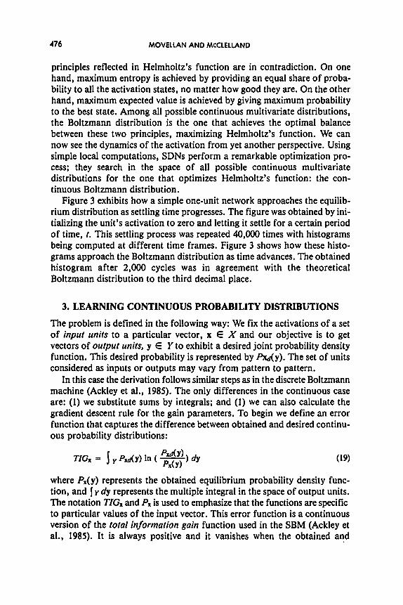
principles reflected in Helmholtz’s function are in contradiction. On one hand, maximum entropy is achieved by providing an equal share of probability to all the activation states, no matter how good they are. On the other hand, maximum expected value is achieved by giving maximum probability to the best state. Among all possible continuous multivariate distributions, the Boltzmann distribution is the one that achieves the optimal balance between these two principles, maximizing Helmholtz’s function. We can now see the dynamics of the activation from yet another perspective. Using simple local computations, SDNs perform a remarkable optimization process; they search in the space of all possible continuous multivariate distributions for the one that optimizes Helmholtz’s function: the continuous Boltzmann distribution.

Figure 3 exhibits how a simple one-unit network approaches the equilibrium distribution as settling time progresses. The figure was obtained by ini- tializing the unit’s activation to zero and letting it settle for a certain period of time, t. This settling process was repeated 40,000 times with histograms being computed at different time frames. Figure 3 shows how these histograms approach the Boltzmann distribution as time advances. The obtained histogram after 2,000 cycles was in agreement with the theoretical Boltzmann distribution to the third decimal place.

3. LEARNING CONTINUOUS PROBABILITY DISTRIBUTIONS

The problem is defined in the following way: We fix the activations of a set of input units to a particular vector, x E X and our objective is to get vectors of output units, y E Y to exhibit a desired joint probability density function. This desired probability is represented by my). The set of units considered as inputs or outputs may vary from pattern to pattern.

In this case the derivation follows similar steps as in the discrete Boltzmann machine (Ackley et al., 1985). The only differences in the continuous case are: (1) we substitute sums by integrals; and (1) we can also calculate the gradient descent rule for the gain parameters. To begin we define an error function that captures the difference between obtained and desired continuous probability distributions:

where P,(y) represents the obtained equilibrium probability density function, and j y & represents the multiple integral in the space of output units. The notation TIG, and Px is used to emphasize that the functions are specific to particular values of the input vector. This error function is a continuous version of the total information gain function used in the SBM (Ackley et al., 1985). It is always positive and it vanishes when the obtained and


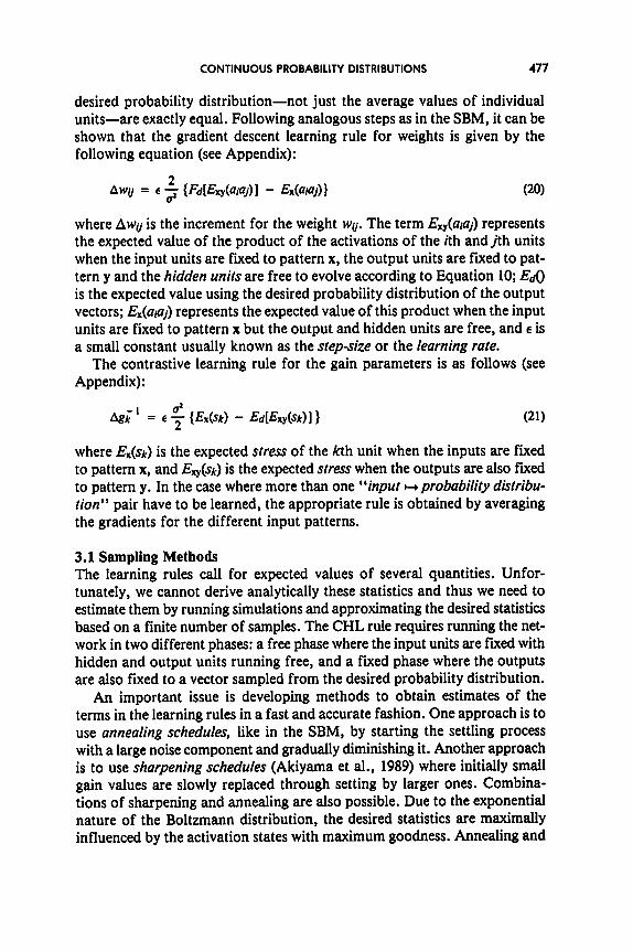
desired probability distribution-not just the average values of individual units-are exactly equal. Following analogous steps as in the SBM, it can be shown that the gradient descent learning rule for weights is given by the following equation (see Appendix):

AWU = 6 $ {F&%y(W/)] - Ex(W~)} (20)

where Awu is the increment for the weight wu. The term .&(Wj) represents the expected value of the product of the activations of the ith andjth units when the input units are fixed to pattern x, the output units are fixed to pattern y and the hidden units are free to evolve according to Equation 10; I%() is the expected value using the desired probability distribution of the output vectors; E,(uia/) represents the expected value of this product when the input units are fixed to pattern x but the output and hidden units are free, and e is a small constant usually known as the step-size or the learning rate.

The contrastive learning rule for the gain parameters is as follows (see Appendix):

where E&k) is the expected stress of the kth unit when the inputs are fixed to pattern x, and &(s~) is the expected strm when the outputs are also fixed to pattern y. In the case where more than one “input wprobability distribution” pair have to be learned, the appropriate rule is obtained by averaging the gradients for the different input patterns.

3.1 Sampling Methods The learning rules call for expected values of several quantities. Unfor- tunately, we cannot derive analytically these statistics and thus we need to estimate them by running simulations and approximating the desired statistics based on a finite number of samples. The CHL rule requires running the network in two different phases: a free phase where the input units are fixed with hidden and output units running free, and a fixed phase where the outputs are also fixed to a vector sampled from the desired probability distribution.

An important issue is developing methods to obtain estimates of the terms in the learning rules in a fast and accurate fashion. One approach is to use annealing schedules, like in the SBM, by starting the settling process with a large noise component and gradually diminishii it. Another approach is to use sharpening schedules (Akiyama et al., 1989) where initially small gain values are slowly replaced through setting by larger ones. Combina- tions of sharpening and annealing are also possible. Due to the exponential nature of the Boltzmann distribution, the desired statistics are maximally influenced by the activation states with maximum goodness. Annealing and

478 MOVELIAN AND MCCLELLAND

sharpening methods try to focus the sampling time to the largest attractors (maxima in the Goodness function) avoiding smaller attractors. However, these procedures run into problems when the network has to learn probability distributions where there is more than one equally desirable pattern of activation for the same input. In this case each of the desired patterns will have a corresponding maximum with the same goodness value. Because annealing schedules are designed to visit only one of the maxima at a time, the obtained statistics will be unstable and will lead to instabilities in the learning process.

In such cases, we have found it beneficial to let the network visit several large attractors before changing the weights. We could achieve this by doing either one of two things: We could let the network settle once per learning trial, giving enough time at equilibrium to jump out of attractors and visit several different ones. We could also restart the network several times from different random points, but with less time at equilibrium each time. In this case the probability of visiting different attractors is obtained by averaging over the several restarts. Since the network is ergodic, equilibrium statistics using one or many restarts converge, but in practice we have found that the stochastic equilibrium statistics are approximated faster by using the multiple restarts method. A similar effect may be achieved by changing the weights based on a temporal moving average of the gradients obtained in previous learning epochs. In our simulations we used the multiple restarts technique in combination with an exponential moving average technique. We did not use annealing or sharpening schedules.

4. SIMUL~IONS

Here we will focus on the CHL rule and the problem of learning discrete and continuous distributions of various types. We present simulations of the four following problems:

1. Completion exclusive-or (XOR): A variation on a standard benchmark for connectionist networks.

2. Word translation problem: Learning bidirectional stochastic mappings of discrete multidimensional representations.

3. Multidimensional continuous probability distributions: Learning various types of multidimensional continuous distributions with and without interdependencies in the output units.

4. XOR governed probability distributions: A problem that requires learning high-order output-unit statistics, and the use of hidden unis.

Results on some of these problems with a previous model instantiating the principles of continuous, stochastic, interactive processing are also presented in Movellan and McClelland (in press).


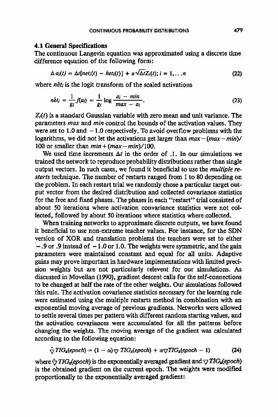
4.1 General Specifications The continuous Langevin equation was approximated using a discrete time difference equation of the following form:

AU&) = At[neti(l) - riet,(t)] + a&?Zzi(t); i = 1,. . .PI (=I where 6ti is the logit transform of the scaled activations

Z(t) is a standard Gaussian variable with zero mean and uriit variance. The parameters max and min control the bounds of the activation values. They were set to 1 .O and - 1 .O respectively. To avoid overflow problems with the logarithms, we did not let the activations get larger than mux- (ma- min)/ 100 or smaller than min + (ma- min)/lOO.

We used time increments At in the order of .l. In our simulations we trained the network to reproduce probability distributions rather than single output vectors. In such cases, we found it beneficial to use the multiple restarts technique. The number of restarts ranged from 1 to 80 depending on the problem. In each restart trial we randomly chose a particular target output vector from the desired distribution and collected covariance statistics for the free and fixed phases. The phases in each “restart” trial consisted of about 50 iterations where activation convariance statistics were not collected, followed by about 50 iterations where statistics where collected.

When training networks to approximate discrete outputs, we have found it beneficial to use non-extreme teacher values. For instance, for the SDN version of XOR and translation problems the teachers were set to either - .9 or .9 instead of - 1 .O or 1 .O. The weights were symmetric, and the gain parameters were maintained constant and equal for all units. Adaptive gains may prove important in hardware implementations with limited preci- sion weights but are not particularly relevent for our simulations. As discussed in Movellan (1990), gradient descent calls for the self-connections to be changed at half the rate of the other weights. Our simulations followed this rule. The activation covariance statistics necessary for the learning rule were estimated using the multiple restarts method in combination with an exponential moving average of previous gradients. Networks were allowed to settle several times per pattern with different random starting values, and the activation covariances were accumulated for all the patterns before changing the weights. The moving average of the gradient was calculated according to the following equation:

-$ TIG,(epoch) = (1 - a))~ TIG,(epoch) + avTIGx(epoch - 1) (24)

where + TIG~epoch) is the exponentially averaged gradient and v 27Gdepoch) is the obtained gradient on the current epoch. The weights were modified proportionally to the exponentially averaged gradient:


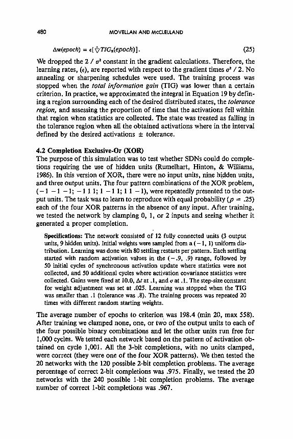
Aw(epoch) = E[ +TIGx(epoch)]. (25)

We dropped the 2 / a2 constant in the gradient calculations. Therefore, the learning rates, (E), are reported with respect to the gradient times 02 / 2. No annealing or sharpening schedules were used. The training process was stopped when the total information gain (TIG) was lower than a certain criterion. In practice, we approximated the integral in Equation 19 by defin- ing a region surrounding each of the desired distributed states, the tolerance region, and assessing the proportion of time that the activations fell within that region when statistics are collected. The state was treated as falling in the tolerance region when all the obtained activations where in the interval defined by the desired activations f tolerance.

4.2 Completion Exclusive-Or (XOR) The purpose of this simulation was to test whether SDNs could do completions requiring the use of hidden units (Rumelhart, Hinton, & Williams, 1986). In this version of XOR, there were no input units, nine hidden units, and three output units. The four pattern combinations of the XOR problem, (-1 -1 -1; - 1 1 1; 1 - 1 1; 1 1 -l), were repeatedly presented to the output units. The task was to learn to reproduce with equal probability (p = .25) each of the four XOR patterns in the absence of any input. After training, we tested the network by clamping 0, 1, or 2 inputs and seeing whether it generated a proper completion.

Specifications: The network consisted of 12 fully connected units (3 output units, 9 hidden units). Initial weights were sampled from a (- 1, 1) uniform distribution. Learning was done with 80 settling restarts per pattern. Each settling started with random activation values in the (- .9, .9) range, followed by 50 initial cycles of synchronous activation update where statistics were not collected, and 50 additional cycles where activation covariance statistics were collected. Gains were fixed at 10.0, At at .l, and u at .l. The step-size constant for weight adjustment was set at .025. Learning was stopped when the TIG was smaller than .1 (tolerance was .8). The training process was repeated 20 times with different random starting weights.

The average number of epochs to criterion, was 198.4 (min 20, max 558). After training we clamped none, one, or two of the output units to each of the four possible binary combinations and let the other units run free for 1,000 cycles. We tested each network based on the pattern of activation obtained on cycle 1,001. All the 3-bit completions, with no units clamped, were correct (they were one of the four XOR patterns). We then tested the 20 networks with the 120 possible a-bit completion problems. The average percentage of correct Zbit completions was .975. Finally, we tested the 20 networks with the 240 possible l-bit completion problems. The average number of correct l-bit completions was .967.


Word Translation Problem

“Spanish” Module

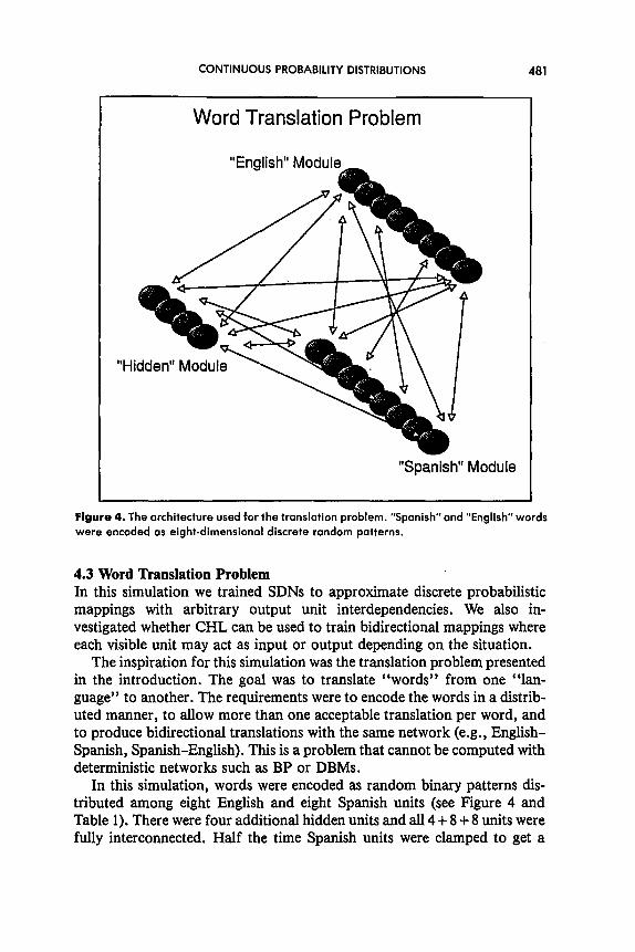
Figure 4. The architecture used for the translation problem. “Spanish” and “English” words were encoded as eight-dimensional discrete random patterns.

4.3 Word Translation Problem In this simulation we trained SDNs to approximate discrete probabilistic mappings with arbitrary output unit interdependencies. We also in- vestigated whether CHL can be used to train bidirectional mappings where each visible unit may act as input or output depending on the situation.

The inspiration for this simulation was the translation problem presented in the introduction. The goal was to translate “words” from one “language” to another. The requirements were to encode the words in a distributed manner, to allow more than one acceptable translation per word, and to produce bidirectional translations with the same network (e.g., English- Spanish, Spanish-English). This is a problem that cannot be computed with deterministic networks such as BP or DBMS.

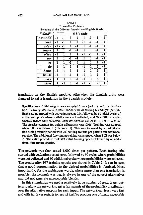
In this simulation, words were encoded as random binary patterns distributed among eight English and eight Spanish units (see Figure 4 and Table 1). There were four additional hidden units and all 4 + 8 + 8 units were fully interconnected. Half the time Spanish units were clamped to get a


TABLE 1 Translation Problem:

Encoding of the Different Spanish and English Words

t olive 1 1 -1 1 -1 -1 -1 1 1

translation in the English module; otherwise, the English units were clamped to get a translation in the Spanish module.

Speclficatlons: Initial weights were sampled from a ( - 1, 1) uniform distribution. Learning was done in batch mode with 20 settling restarts per pattern. Each settling started with activations set at 0.0, followed by 50 initial cycles of activation update where statistics were not collected, aqd 50 additional cycles where statistics were collected. Gain was fixed at 1 .O, At at .l, u at .l, cx at .4. The stepsize constant for weight adjustment was .0025. Training was stopped when TIG was below .I (tolerance .8). This was followed by an additional fine-tuning training period with 200 settling restarts per pattern (40 additional epochs). The additional fine-tuning training was stopped when TIG was below . 1. The entire procedure took 927 initial training epochs followed by 40 additional fine-tuning epochs.

The network was then tested 1,000 times per pattern. Each testing trial started with activations set at zero, followed by 50 cycles where probabilities were not collected and 50 additional cycles where probabilities were collected. The results after 967 training epochs are shown in Table 2. It can be seen that a good approximation to the desired probabilities is obtained. Most importantly, for the ambiguous words, where more than one.translation is possible, the network was nearly always in one of the correct alternatives and did not generate unacceptable blends.

In this stimulation we used’a relatively large number of restarts per pattern to allow the network to get a fair sample of the probability distribution over the alternative outputs for each input. The network can learn very fast and with far fewer restarts to restrict itself to produce one of many acceptable


TABLE 2 Translation Problem

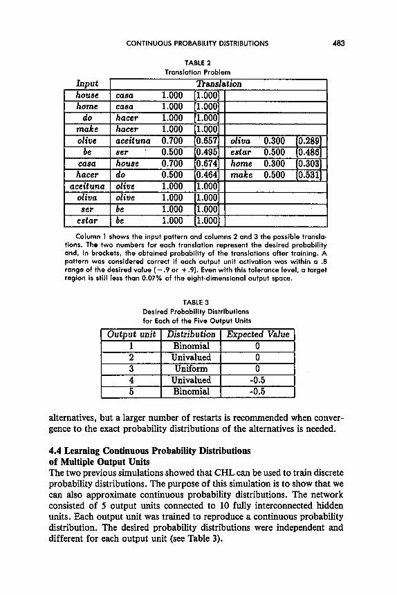
Input Tkanslation casa 1.000 [l.OOO] casa 1.000 [l.OOO] hater 1.000 [l.OOO] hater 1.000 [l.OOO] aceituna 0.700 [0.657] oliva 0.300 to.2891 ser 0.500 [0.495] estar 0.500 [0.486] house 0.700 [0.674] home 0.300 [0.303] do 0.500 [0.464] make 0.500 [0.531] olive 1.000 [l.OOO] olive 1.000 [l.OOO] be 1.000 [l.OOO] be 1 .ooo [l .OOO]

Column 1 shows the input pattern and columns 2 and 3 the possible translations. The two numbers for each translation represent the desired probability and, in brackets, the obtained probability of the translations after training. A pottern was considered correct if each output unit activation wos within a .B range of the desired value (- .9 or + .9). Even with this tolerance level, a target region is still less than 0.07% of the eight-dimensional output space.

[ estar

TABLE 3

Desired Probability Distributions for Each of the Five Output Units

alternatives, but a larger number of restarts is recommended when conver- gence to the exact probability distributions of the alternatives is needed.

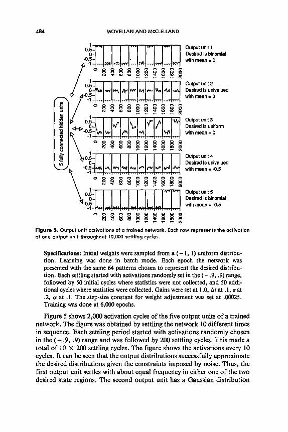
4.4 Learning Continuous Probability Distributions of Multiple Output Units The two previous simulations showed that CHL can be used to train discrete probability distributions. The purpose of this simulation is to show that we can also approximate continuous probability distributions. The network consisted of 5 output units connected to 10 fully interconnected hidden units. Each output unit was trained to reproduce a continuous probability distribution. The desired probability distributions were independent and different for each output unit (see Table 3).


r-T - Output unit 1 Desired is binomial with mean = 0

Output unit 2 Desired is univalued with mean = 0

og~g~~ooooo c.I*wwo 83888 -7-v-v-%-N

Output unit 3 Desired is uniform with mean = 0

0888gogoggo NWWW -YrrrN 8 3ww8

Output unit 4 Desired is univalued

~2y+4h*~I+u3d with mean = -0.5

v-t-%-N - Output unit 5

Desired is binomial with mean = -0.5

0888888O888 N*ww~~ 8 w m 0 V-r-N Figure 5. Output unit activations of a troined network. Each row represents the activation of one output unit throughout 10,000 settling cycles.

Specifications: Initial weights were sampled from a (- 1, 1) uniform distribution. Learning was done in batch mode. Each epoch the network was presented with the same 64 patterns chosen to represent the desired distribution. Each settling started with activations randomly set in the (- .9, .9) range, followed by 50 initial cycles where statistics were not collected, and 50 additional cycles where statistics were collected. Gains were set at 1 .O, AI at .l, u at .2, o! at .l. The step-size constant for weight adjustment was set at .00025. Training was done at 6,000 epochs.

Figure 5 shows 2,000 activation cycles of the five output units of a trained network. The figure was obtained by settling the network 10 different times in sequence. Each settling period started with activations randomly chosen in the (- .9, .9) range and was followed by 200 settling cycles. This made a total of 10 x 200 settling cycles. The figure shows the activations every 10 cycles. It can be seen that the output distributions successfully approximate the desired distributions given the constraints imposed by noise. Thus, the first output unit settles with about equal frequency in either one of the two desired state regions. The second output unit has a Gaussian distribution


@!kmc?~T-c?roko! ??P?P~~OOO

Acllvatlon

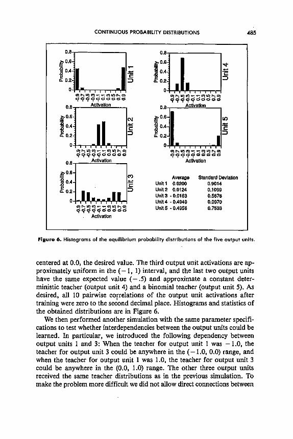
Average Standard Deviation Unit 1 0.0200 0.9014 Unit 2 0.0124 0.1099 Unit 3 - 0.0163 0.5676 Unit 4 - 0.4949 0.0970

- Unit 5 0.4956 0.7633

Figure 6. Histograms of the equilibrium probability distributions of the five output units.

centered at 0.0, the desired value. The third output unit activations are approximately uniform in the (- 1, 1) interval, and the last two output units have the same expected value (- .5) and approximate a constant deterministic teacher (output unit 4) and a binomial teacher (output unit 5). As desired, all 10 pair-wise cofrelations of the output unit activations after training were zero to the second decimal place. Histograms and statistics of the obtained distributions are in Figure 6.

We then performed another simulation with the same parameter specifications to test whether interdependencies between the output units could be learned. In particular, we introduced the following dependency between output units 1 and 3: When the teacher for output unit 1 was - 1.0, the teacher for output unit 3 could be anywhere in the (- 1 .O, 0.0) range, and when the teacher for output unit 1 was 1.0, the teacher for output unit 3 could be anywhere in the (0.0, 1.0) range. The other three output units received the same teacher distributions as in the previous simulation. To make the problem more difficult we did not allow direct connections between

486

Output unit 1 Desired is blnomlal with mean - 0

500 1000 1500 2000

9, ~ , , I- :vmj Outputunit

0 500 1000 1500 2000

MOVELLAN AND MCCLELLAND

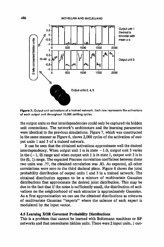
Figure 7. Output unit octivatians of a trained network. Each row represents the activations

of each output unit throughout 10,000 settling cycles.

the output units so that interdependencies could only be captured via hidden unit connections. The network’s architecture and the learning parameters were identical to the previous simulations. Figure 7, which was constructed in the same manner as Figure 6, shows 2,000 cycles of the activation of output units 1 and 3 of a trained network.

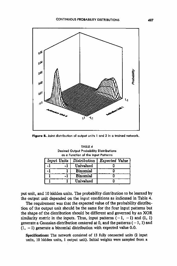
It can be seen that the obtained activations approximate well the desired interdependency. When output unit 1 is in state - 1.0, output unit 3 varies in the (- 1,O) range and when output unit 1 is in state 1, output unit 3 is in the (0, 1) range. The expected Pearson correlation coefficient between these two units was .77, the obtained correlation was .83. As expected, all other correlations were zero to the third decimal place. Figure 8 shows the joint probability distribution of output units 1 and 3 in a trained network. The obtained distribution appears to be a mixture of multivariate Gaussian distributions that approximate the desired joint distribution. This may be due to the fact that if the noise is sufficiently small, the distribution of activations on the neighborhood of each attractor is approximately Gaussian. As a first approximation we can see the obtained distributions as mixtures of multivariate Gaussian “experts” where the salience of each expert is modulated by the input vector.

4.5 Learning XOR Governed Probability Distributions This is a problem that cannot be learned with Boltzmann machines or BP networks and that necessitates hidden units. There were 2 input units, 1 out-


Figure 8. Joint distribution of output units 1 ond 3 in a troined network.

TABLE 4 Desired Output Probability Distributions

OS o Function of the Input Potterns

put unit, and 10 hidden units. The probability distribution to be learned by the output unit depended on the input conditions as indicated in Table 4.

The requirement was that the expected value of the probability distribution of the output unit should be the same for the four input patterns but the shape of the distribution should be different and governed by an XOR similarity metric in the inputs. Thus, input patterns (- 1, - 1) and (1, 1) generate a Gaussian distribution centered at 0, and the patterns (- 1, 1) and (1, - 1) generate a binomial distribution with expected value 0.0.

Specifications: The network consisted of 13 fully connected units (2 input units, 10 hidden units, 1 output unit). Initial weights were sampled from a


0.6 0.6

0.4 go.4

: 0.2 g 3 0.2

0 0 Tk?~TT~Yh? ?PP?Q*****

Aotivatlon Aotivatlon

0.6 0.6

p 0.4 1 iioe4

B 0.2 f 0.2

0 0

'?'???Qooooo QQQQQooo"* Activation Activation

Desired Dislributlon

Obtained Dlstrbutbn

Figure 9. Desired and obtained probability distributions in the output unit as o response to the four different input potterns.

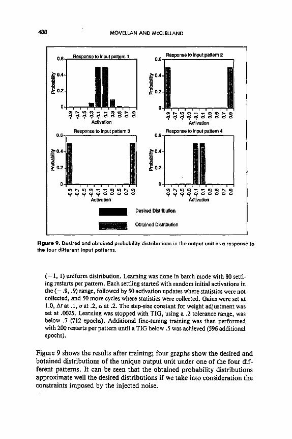
(- 1, 1) uniform distribution. Learning was done in batch mode with 80 settling restarts per pattern. Each settling started with random initial activations in the (- .9, .9) range, followed by 50 activation updates where statistics were not collected, and 50 more cycles where statistics were collected. Gains were set at 1 .O, At at .I, u at .2, a! at .2. The step-size constant for weight adjustment was set at 4025. Learning was stopped with TIG, using a .2 tolerance range, was below .7 (712 epochs). Additional fine-tuning training was then performed with 200 restarts per pattern until a TIG below .S was achieved (596 additional epochs).

Figure 9 shows the results after training; four graphs show the desired and botained distributions of the unique output unit under one of the four different patterns. It can be seen that the obtained probability distributions approximate well the desired distributions if we take into consideration the constraints imposed by the injected noise.


5. DISCUSSION

The work presented above builds on earlier work on discrete stochastic networks (Ackley et al., 1985; Geman & Geman, 1984; Smolensky, 1986) and extends this previous work to the continuous diffusion case (SDN). First, we showed that the equilibrium probability distribution of SDNs is continuous Boltzmann. This significant result is easily derivable from Markovian diffusion theory, but to our knowledge, had not been previously presented. Most importantly, this result holds for other bounded dynamical systems whose time derivatives are the gradient of an objective function (the drift) and additive Gaussian noise (the diffusion). This may have important impli- cations for general optimization of continuous functions with known derivatives. For example, the error function used in back propagation learning (TSS) could play the same role as the goodness function in SDNs. If we add Gaussian noise to the gradient of TSS with respect to weights, we would also obtain a Markovian diffusion system. The evolution of the probability distribution of the weights would then be determined by a Fokker-Planck equation analogous to 10, but substituting activations by weights and goodness, G(a), by - TSS(w). If the weights are bounded, the noisy version of the back propagation rule would exhibit a Boltzmann equilibrium distribution in weight space. Using a sufficiently slow annealing schedule we could then guarantee achievement of global minima in weight space.

With respect to learning, we have focused on the CHL rule and its ability to learn entire distributions. We have shown that when applied to SDNs, it performs gradient descent on the total information gain error function (TIG). This function captures differences between desired and obtained continuous multivariate probability distributions beyond expected values and vanishes only when obtained and desired probability distributions are equal. Simulations were used to show that, indeed, CHL can be used to approximate discrete probability distributions, continuous probability distributions, and deterministic input-output mappings.

Considerable work remains to be done. We need to try CHL with larger problems. In its present form CHL learns very quickly in terms of number of epochs but the processes of estimating the gradients may take thousands of cycles. Developing fast methods to estimate the desired gradients will be a major prerequisite for the development of practical applications. In our simulations we have used temporal averaging of the gradients to speed up learning. We suspect that the spatial averaging that goes on in natural nervous systems may also have positive effects. We believe that the multiple restarts technique, which we used in our simulations, may serve a similar purpose to this spatial averaging. The learning algorithm and the activation dynamics can also be optimized with massively parallel architectures or with VLSI implementations. In this respect the chip developed at Bellcore


(Alspector, Jayakumar, & Luna, 1992) is a promising possibility. In its present form it can implement a 32-unit SDN-style network trained with the CHL algorithm at a speed of 100,000 input-output patterns per second.

We believe that SDNs may excel in applications that take full advantage of the principles of continuous, stochastic, and interactive processing. Ran- domness and graded activations allow learning continuous probability distributions where the same input may have more than one acceptable output; noise is essential here, rather than simply being a hindrance. Stochastic diffusion networks may also prove useful in other kinds of learning para- digms as well. CHL is based on minimization of the TIG, a very general error function. This makes CHL very general and capable of learning entire probability distributions. In practice though, rules based on minimization of less general error functions-such as TSS or the probability of being wrong- may have advantages in particular learning situations. We have derived such learning rules and we are presently comparing their performance with the CHL rule.

Theoretically, we need to address important issues regarding the learning, representational, and dynamical behavior of these networks: How many probability distributions can be learned? What kind of problems are learnable with the different algorithms? Are these networks subject to catastrophic interference? Are they universal contingency approximators? Do they exhibit well-known phenomena from the human cognition litera- ture? Can we extend the learning algorithm to the more general case of learning probabilistic sequences?

The capacity of SDNs to tackle very general forms of contingency extends the possibilities of adaptive networks to model learning and development. The capacity of infants to detect contingencies hasplayed an important role in many theories of development. Aspects such as the development of cross- modal representations and symbolic reference (Piaget, 1936), the development of reaching and object permanence (Piaget, 1937), and early social development (Watson, 1985) have been linked to the infant’s capacity to detect contingencies. Yet, very few theories pay attention to the types of contingencies underlying these problems and the mechanisms necessary to learn them. For example, only recent articles (Jordan, 1989; Jordan & Rumelhart, 1992) have addressed the averaging problem that exists when learning how to reach. The capacity of SDNs to detect a very wide variety of contingencies that go beyond expected values may help us explore aspects of development that were not easily approached with other adaptive networks.

Most importantly, symmetric diffusion networks may help expand our notions of how natural nervous systems may represent information. In deterministic networks, the activation states can be seen as internal representations of the inputs, and the maxima in the goodness function as interpretations the network settles into. This approach illustrates how


cognitive schemas could emerge from the interaction of interconnected units (Rumelhart, Smolensky, & McClelland, 1986). Stochastic networks (i.e., the SBM, the harmonium, and SDNs) take us a step further. Their behavior can only be stated in terms of probabilities, and their stable states are no longer activation vectors but probability distributions. In spite of the fact that the activation states are constantly changing, there is an underlying in- variant: the particular way in which probability density spreads through the different states. In SDNs this evolution is governed by the forward diffusion equation, and culminates in stochastic equilibrium. This underlying structure may not be detected directly in a single observation, but it is_ reflected when sampling the network’s response over many trials. As Ackley et al., (1985) noted, the late von Neumann (1958) thought of stochasticity as an essential principle that differentiated the digital computer from the brain. He suggested that noise may not be a hindrance in natural nervous systems, but an essential information-processing principle:

. . . the message-system used in the nervous system. . . is of an essentially statrkti- cal character. . . . Thus the nervous system appears to be using a radically different system of notation from the ones we are familiar with in ordinary arith- metic and mathematics: instead of the precise system of markers where the position-and presence or absence-of every marker counts decisively in determining the meaning of the message, we have here a system of notations in which the meaning is conveyed by the statistical properties of the message. (von Neumann, 1958, p. 79)

It is hoped that SDNs will help in developing models of cognition to understand better the computational properties of stochastic distributed representations.

In the past, since most emphasis was given to learning speed, and since simulating randomness greatly slowed down learning, stochastic networks and the problem of learning probability distributions were somehow for- gotten. We hope our work helps to emphasize the possibilities of stochastic networks and the importance of learning contingencies that involve complete real-valued probability distributions.

REFERENCES

Ackley, D., Hinton, G., & Sejnowski, T. (1985). A learning algorithm for Boltzmann machines. Cogntive Science, 9, 147-169.

Alspector, J., Jayakumar, A., & Luna, S. (1992). Experimental evaluation of learning in a neuronal mycrosystem. In J. Moody, S. Hanson, & R. Lippmann. Advances in neurul information processing systems. (Vol. 4).

Akiyama, Y., Yamashita, A., Kajiura, M., & Aiso, H. (1989). Combinatorial optimization with Gaussian Machines. Proceedings of the Znternotional Joint Cortference on Neural Networks 1, 533-540.

Baldi, P., & Pineda, F. (1991). Contrastive learning and neural oscillations. NeuralComputation, 3(4), 524-545.


Bryson, A., & Ho, Y. (1969). Applied oplimal control. New York: Blaisdell. Galland, C., & Hinton, G. (1989). Deterministic Boltzmann Learning in networks with asym-

metric connectivity. Department of Computer Science, University of Toronto. (Tech. Rep. No. CRG-TR-89-6).

Gardiner, C.W. (1985). Handbook of Stochastic Methods for Physics, Chemistry and the Natural Sciences. Berlin: Springer-Verlag.

Geman, S., L Geman, D. (1984). Stochastic relaxation: Gibbs distributions and the Bayesian restoration of images. IEEE Transactions on Patterns Analysis and Machine Intelli- gence, 6, 721-741.

Gillespie, D. (1992). Markov processes: An introduction for Physical Scientists. San Diego: Academic.

Hinton, G.E. (1989). Deterministic Boltzmann learning performs steepest descent in weight- space. Neural Computation, I, 143-150.

Hopfield, J., Feinstein, D., & Palmer, R. (1983). Unlearning has a stabilizing effect in collective memories. Nature, 304, 158-159.

Hopfield, J. (1984). Neurons with graded response have collective computational properties like those of two-state neurons. Proceedings of the National Academy of Sciences USA, 81, 3088-3092.

Jordan, J. (1989). Motor learning and the degrees of freedom problem. In M. Jeannerod (Ed.). Attention and performance. Hillsdale: Erlbaum.

Jordan, M., & Rumelhart, D. (1992). Forward models: Supervised learning with a distal teacher. Cognitive Science, 16, 307-354.

Le Curt, Y. (1985). Une Procedure d’apprentissaage pour reseau a seuil assymetrique. In Cognitiva 85: A la frontiere de I’intelligence artificielle des sciences de al connaissance des neurosciences. Paris, 599-604.

McClelland, J., & Rumelhart, D. (1981). An interactive activation model of context effects in letter perception: Part 1. An account of basic findings. Psychological Review, 88, 5.

McClelland, J. (1993). Toward a theory of information processing in graded random interactive networks. In Allenlion and Performance (Vol. 14, pp. 655-689). Cambridge, MA.

Metropolis, N., Rosenbluth, A., Rosenbluth, M., Teller, A., &Teller, E. (1953). Equations of state calculations for fast computing machines. Journal of Chemical Physics, 6, 1087.

Movellan, J. (1990). Contrastive Hebbian learning in the continuous Hopfleld model. In D. Touretzky, J. Elman, T. Sejnowski, & G. Hinton: Connectionist models: Proceed- ings of the 1990 Summer School. San Mateo: Morgan Kauffmann.

Movellan, J., & McClelland, J. (in press). Contrastive learning with graded random networks, In T. Petsche (Ed.) Computational learning theory and natural learning systems (Vol. Z), Cambridge, MA: MIT Press.

Papoulis, A. (1990). Probability and statistics. Englewood Cliffs, NJ: Prentice-Hall. Parker, D. (1985). Learning logic. Technical report TR-47, Center for computational research

in economics and management science. MIT Press. Peterson, C., & Anderson, J. (1987). A mean field theory learning algorithm for neural net-

works. Complex Systems, 1. 995-1019. Peterson, C., & Hartman, E. (1989). Explorations of the Mean Field Theory Learning Algo-

rithm. Neural Networks, 2, 475-494. Piaget, J. (1936). Origins of intelligence in children. New York: International University Press. Piaget, J. (1937). The construction of reality in the child. London: Routledge and Kegan Paul. Pomerleau, D. (1991). Efficient training of artificial neural networks for autonomous naviga-

tion. Neural Computalion. 3, 88-98. Ratcliff, R. (1978). A theory of memory retrieval. Psychological Review, 85, 59-107. Rumelhart, D., Hinton, G., & Williams, R. (1986). Learning internal representation by error

propagation. In D. Rumelhart 8r J.L. McClelland (Eds.), Parallel distributedprocess- ing: Exploralions in the microstructure of cognition. Volume I: Foundations. Cam- bridge, MA: MIT Press.


Rumelhart, D., Smolensky, P., McClelland, J., & Hinton, Cl. (1986). Schemata and sequential thought processes in PDP models. In J. McClelland & D. Rumelhart (Eds.), Purullel distributed processing: Explorations in the microstructure of cognition. Volume 2: Psychological und biological models. Cambridge, MA: MIT Press.

Smolensky, P. (1986). Information Processing in dynamical systems: Foundations of harmony theory. In D. Rumelhart, & J.L. McClelland (Eds.), Parallel distributed processing: Explorations in the microstructure of cognition. Volume I: Foundatidns. Cambridge, MA: MIT Press.

Taylor, I., Jr Karlin, S. (1984). An introduction to stochastic modeling. Orlando: Academic. von Neumann, J. (1958). The computer and the brain. New Haven: Yale University Press. Watson, J. (1985). Contingency perception in early social development. In T.M. Field &

N.A. Fox (Eds.). Socialperception in infants, Norwood, NJ: Ablex. Werbos, P. (1974). Beyond regression: New tools for prediction and analysis in the behavioral

sciences. Unpublished doctoral dissertation, Harvard University, Boston.

6. APPENDIX

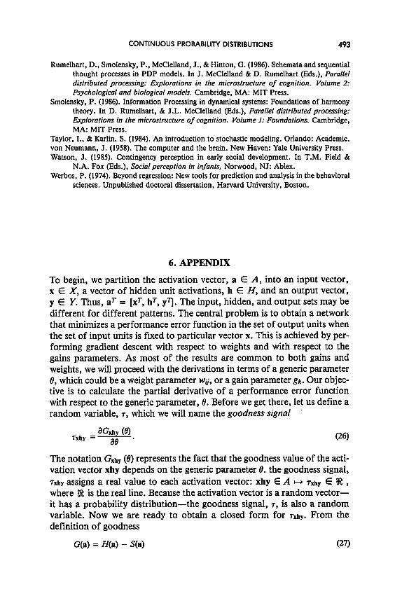
To begin, we partition the activation vector, a E A, into an input vector, x E X, a vector of hidden unit activations, h E H, and an output vector, y E Y. Thus, aT = [xr, hT, ~1. The input, hidden, and output sets may be different for different patterns. The central problem is to obtain a network that minimizes a performance error function in the set of output units when the set of input units is fixed to particular vector x. This is achieved by per- forming gradient descent with respect to weights and with respect to the gains parameters. As most of the results are common to both gains and weights, we will proceed with the derivations in terms of a generic parameter 0, which could be a weight parameter wg, or a gain parameter gk. Our objective is to calculate the partial derivative of a performance error function with respect to the generic parameter, 8. Before we get there, let us define a random variable, 7, which we will name the goodness signal

Txhy = =XIIY (‘4

ae * The notation Gxhy (19) represents the fact that the goodness value of the activation vector xhy depends on the generic parameter 8. the goodness signal, rxhy assigns a real value to each activation vector: xhy E A H 7xby E ‘W , where $I is the real line. Because the activation vector is a random vector- it has a probability distribution-the goodness signal, 7, is also a random variable. Now we are ready to obtain a closed form for 7xhy. From the definition of goodness

G(a) = H(a) - S(a) (27)


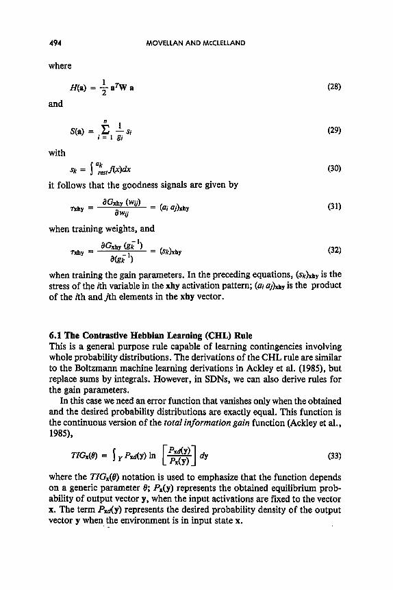
where

H(a) = -+a and

with Sk = s u~,m~

it follows that the goodness signals are given by

7xhy = aGfiy (wd = (& aj)* awii Y

when training weights, and -1

=xhy &k ) Txhy =

a(6 ‘1 = bk)xhy (32)

when training the gain parameters. In the preceding equations, (sk)xhy is the stress of the ith variable in the xhy activation pattern; (Ui aJxhy is the product of the ith and&h elements in the xhy vector.

6.1 The Contrastive Hebbian Learning (CHL) Rule This is a general purpose rule capable of learning contingencies involving whole probability distributions. The derivations of the CHL rule are similar to the Boltzmann machine learning derivations in Ackley et al. (1985), but replace sums by integrals. However, in SDNs, we can also derive rules for the gain parameters.

In this case we need an error function that vanishes only when the obtained and the desired probability distributions are exactly equal. This function is the continuous version of the total information gain function (Ackley et al., 1985),

TIG,(@ = j y P&Y) In c 1 PxdY) & - Px(Y)

where the TIGx(0) notation is used to emphasize that the function depends on a generic parameter 8; Px(y) represents the obtained equilibrium probability of output vector y, when the input activations are fixed to the vector x. The term P&y) represents the desired probability density of the output vector y when the environment is in input state x. _

CONTINUOUS PROBABILITY DISTRIBUTIONS

s $ yPdY) In hdY)l dy - $ +‘x~Y) In Px(Y)I &

and since the first term in Equation 34 is constant, it follows that

aT=x(B) = - ae J y&d(Y) 6 [In WY)1 ti

(34)

(35)

where we need to calculate a / 30 [m P,(y)]. The term&(y) can be found by integrating the network states whose output unit activations coincide with the vector y. Therefore,

px(y) = JHpxo h. (36)

And since the equilibrium distribution is Boltzrnann,

Px(y) = + j H eGxtly~~)~ dh x (37)

where & = 1 y jn eGxhy@$ dhdy is known as the partition constant for the SDN with fixed inputs.

Notice that

PO z jH C?GXh& dh P(YlX) = -=-

P(x) z j y jH eGxhy& dh &’ = Px(Y) (38)

where P(xy) is the probability that a network with all its units running free, including the input units, exhibits an output vector y and an input vector x. The term p(x) is the probability of the input vector x in the totally free running network, P(y(x) is the conditional probability of y with respect to x, andZ= ~Y~HIX emY@)$ dxdhdy is the partition constant for the totally free running network. It follows that

$j (In j H eGxh y(e) f dh)

The first term of the right side in Equation 39 can be expanded as

1 J

2 ac;b,(e) I-

jH ,Oxh& & H &&y@) a db

ae


2 1 =-- d & s H &thy& 7xhy (0) dh

2 =- a’ s H Px,Jh)m,y dh = -+ J%(d (42)

where Z, is the partition constant of an SDN with the inputs and outputs fixed to the vectors x and y respectively; p&h) represents the equilibrium probability of a particular vector of hidden unit activations when the input units are fixed to the input vector x and the output units to the vector y, and I&(r) represents the expected value of the goodness signal rtiy when inputs and outputs are fixed.

Using steps analogous to 40 through 42, it is easy to show that

$ (ln J y S, e%hy@?f dhdy) = $E,(T) where I&(r) represents the expected value of the goodness signal 7xhy when the input units are fiied and the other units run free. Combining Equations 35 and 43 we get the derivative of the logarithm of the probability of output vector y

i [In px(~)l = $ VMd - Ex(dl.

Combining Equation 44 with 38 and 39 we obtain the derivative of the total information gain error function:

aT’.Gx@) =

ae -f{j y PxdY) [~&) - EXWI dY 1

and since the integral in Equation 45 is an expected value operator

B~IG,un = ae

- f {Ed Ey(dl - Ex(d)

where I&o is the expected value using the desired probability distribution of output vectors. When more than one “input wprobability distribution” pair is involved, the appropriate gradient is obtained by averaging over patterns. The gradient descent learning rules for gains and weights easily follow.

Learning Continuous Probability Distributions with

Documents

Transcript of Learning Continuous Probability Distributions with