Learning by Imitation in Games: Theory, Field, and...
75
Learning by Imitation in Games: Theory, Field, and Laboratory Erik Mohlin y Robert stling z Joseph Tao-yi Wang x June 18, 2015 Abstract We exploit a unique opportunity to study how a large population of players in the eld learn to play a novel game with a complicated and non-intuitive mixed strategy equilibrium. We argue that standard models of belief-based learning and reinforcement learning are unable to explain the data, but that a simple model of similarity-based global cumulative imitation can do so. We corroborate our ndings using laboratory data from a scaled-down version of the same game, and demonstrate out-of-sample explanatory power in three other games. The theoret- ical properties of the proposed learning model are studied by means of stochastic approximation. jel classification: C72, C73, L83. keywords: Learning; imitation; behavioral game theory; evolutionary game the- ory; stochastic approximation; replicator dynamic; similarity-based reasoning; gen- eralization; mixed equilibrium. We are grateful for comments from Ingela Alger, Alan Beggs, Ken Binmore, Colin Camerer, Vin- cent Crawford, Ido Erev, David Gill, Yuval Heller, and Peyton Young, as well as seminar audiences at the Universities of Edinburgh, Essex, Lund, Oxford, Warwick and St Andrews, University College London, the 4th World Congress of the Game Theory Society in Istanbul, the 67th European Meeting of the Econometric Society, and the 8th Nordic Conference on Behavioral and Experimental Economics. Kristaps Dzonsons (k -Consulting) and Kaidi Sun provided excellent research assistance. Erik Mohlin acknowledges nancial support from the European Research Council, Grant no. 230251, Robert stling acknowledges nancial support from the Jan Wallander and Tom Hedelius Foundation, and Joseph Tao-yi Wang acknowledges support from the NSC of Taiwan. y Nu¢ eld College and Department of Economics, University of Oxford. Address: Nu¢ eld College, New Road, Oxford OX1 4PX, United Kingdom. E-mail: erik.mohlin@nu¢ eld.ox.ac.uk. z Institute for International Economic Studies, Stockholm University, SE106 91 Stockholm, Sweden. E-mail: [email protected]. x Department of Economics, National Taiwan University, 21 Hsu-Chow Road, Taipei 100, Taiwan. E-mail: [email protected].
Transcript of Learning by Imitation in Games: Theory, Field, and...

Learning by Imitation in Games:Theory, Field, and Laboratory∗
Erik Mohlin† Robert Östling‡ Joseph Tao-yi Wang§
June 18, 2015
Abstract
We exploit a unique opportunity to study how a large population of players inthe field learn to play a novel game with a complicated and non-intuitive mixedstrategy equilibrium. We argue that standard models of belief-based learning andreinforcement learning are unable to explain the data, but that a simple modelof similarity-based global cumulative imitation can do so. We corroborate ourfindings using laboratory data from a scaled-down version of the same game, anddemonstrate out-of-sample explanatory power in three other games. The theoret-ical properties of the proposed learning model are studied by means of stochasticapproximation.
jel classification: C72, C73, L83.keywords: Learning; imitation; behavioral game theory; evolutionary game the-ory; stochastic approximation; replicator dynamic; similarity-based reasoning; gen-eralization; mixed equilibrium.
∗We are grateful for comments from Ingela Alger, Alan Beggs, Ken Binmore, Colin Camerer, Vin-cent Crawford, Ido Erev, David Gill, Yuval Heller, and Peyton Young, as well as seminar audiencesat the Universities of Edinburgh, Essex, Lund, Oxford, Warwick and St Andrews, University CollegeLondon, the 4th World Congress of the Game Theory Society in Istanbul, the 67th European Meetingof the Econometric Society, and the 8th Nordic Conference on Behavioral and Experimental Economics.Kristaps Dzonsons (k -Consulting) and Kaidi Sun provided excellent research assistance. Erik Mohlinacknowledges financial support from the European Research Council, Grant no. 230251, Robert Östlingacknowledges financial support from the Jan Wallander and Tom Hedelius Foundation, and Joseph Tao-yiWang acknowledges support from the NSC of Taiwan.†Nuffi eld College and Department of Economics, University of Oxford. Address: Nuffi eld College,
New Road, Oxford OX1 4PX, United Kingdom. E-mail: erik.mohlin@nuffi eld.ox.ac.uk.‡Institute for International Economic Studies, Stockholm University, SE—106 91 Stockholm, Sweden.
E-mail: [email protected].§Department of Economics, National Taiwan University, 21 Hsu-Chow Road, Taipei 100, Taiwan.
E-mail: [email protected].

1 Introduction
Learning by copying others seems to be prevalent in the animal world as well as in human
societies.1 Copying the successful behavior of others is not only common, but also effec-
tive, when solving individual decision problems.2 It has also been argued that imitation
plays an important role, alongside innovation, when firms develop new products.3 How-
ever, it is less clear how useful imitation is as a learning rule in other strategic settings.4
For example, imitation is likely to be counterproductive in settings where there is a ben-
efit of not behaving like others. Moreover, since it is diffi cult to empirically distinguish
imitative learning from other learning rules, the existing evidence for learning by imita-
tion in games almost exclusively comes from laboratory experiments (e.g. Apesteguia,
Huck and Oechssler, 2007 and Offerman and Schotter, 2009). Consequently, we know
very little about the extent to which imitation is used in human strategic interactions
outside the laboratory.
In this paper, we demonstrate that players do learn by imitation in a field setting
where the game people play is well-defined. In particular, we find strong evidence that
players utilize globally available information in order to imitate strategies that are similar
to previously successful strategies. In both the field setting and in additional laboratory
games, this learning heuristic results in rapid convergence of behavior. Given the abun-
dance of success-oriented information available through the Internet and mass media,
and the pace at which success stories can go viral and spread almost instantaneously, we
believe that the proposed learning model is not limited to its original field setting, but
instead is useful in other settings. Our learning model is particularly well-suited for com-
plex environments in which winner stories are widely available and salient to followers,
whereas other common learning models may not even applicable in such environments.
For example, stories about the relatively small number of successful entrepreneurs are
widely circulated, whereas much less information is available about the majority of en-
1See, for example, Laland (2001) for a discussion of imitation in the animal world, and see section IIIin Armstrong and Huck (2010) for a survey of some relevant research in economics.
2In the context of a fixed set of multi-armed bandits, Schlag (1998) shows that in a class of learningrules with limited memory, which are based on pair-wise comparisons, imitation beats all other learningrules. In a recent tournament organized by evolutionary biologists, learning algorithms heavily basedon imitation proved to be most successful in solving a complex and dynamically changing multiarmedbandit problem (Rendell, Boyd, Cownden, Enquist, Eriksson, Feldman, Fogarty, Ghirlanda, Lilicrap andLaland, 2010).
3In an early but influential research, Urban, Gaskin and Mucha (1986) reported the second entrantearning 71% of the share of the pioneer, which is substantial since they have lower innovation costs.They also suggested introducing unique features to surpass the pioneer, which is indeed the case of IBM,Apple, Wal-Mart, and so on (Shenkar, 2010).
4Duersch, Oechssler and Schipper (2012) show that a simple “imitate-the-best”learning rule cannotbe beaten by any other type of learning rule (including rational and forward-looking behavior) in mostsymmetric two-player games. In other games, like rock-papers-scissors, however, imitating players caneasily be exploited by the opponent. As we will see, the game studied in this paper, LUPI, has a structurethat is similar to that of rock-papers-scissors. Still, the large number of strategies and payoffs in practicemakes it very diffi cult to exploit a population of imitators in LUPI.
1

trepreneurs that failed (or did not even get started).
The field game studied in this paper is the lowest unique positive integer (LUPI)
game introduced by Östling, Wang, Chou and Camerer (2011). In the LUPI game,
players simultaneously choose positive integers from 1 to K and the winner is the player
who chooses the lowest number that nobody else picked. There are several advantages of
using the LUPI data to study strategic learning. The same strategic game was played for
49 consecutive days which allows for learning in a stable strategic environment. The game
has simple and clear rules, yet the theoretical prediction for the game is a complicated
unique mixed strategy equilibrium which is very diffi cult to compute. Most likely no
player could figure out the equilibrium and therefore had to resort to some other heuristic
to guide their behavior. In addition, the game exactly resembles few other strategic
situations, which allows us to study the behavior of truly inexperienced players who are
unlikely to be tainted by preconceived ideas formed in other similar interactions.5
Östling et al. (2011) showed that play in the LUPI game quickly comes surprisingly
close to the equilibrium prediction (although it does not quite converge to equilibrium
in 49 rounds). Similarly, in a scaled-down and simplified laboratory version of the field
game, there is rapid movement toward equilibrium. In this paper we take on the task
explaining why this happens, and what it implies for theories of learning more generally.6
Since the learning model we propose was devised after observing the LUPI data, we also
study the model’s out-of-sample explanatory power in three additional games played in
the laboratory.
Explaining rapid movement toward the equilibrium of the LUPI game is challenging
for traditional models of learning. Reinforcement learning, i.e. learning based on rein-
forcement of chosen actions (e.g. Cross, 1973, Arthur, 1993, and Roth and Erev, 1995), is
far too slow to explain the observed behavior in the field game. The reason is that most
players never win, and hence, their actions are never reinforced. Reinforcement learning
is somewhat more successful in the laboratory game, but as we show below, it is consis-
tently outperformed by our own model of learning by imitation. The leading example
of belief-based learning, fictitious play (see e.g. Fudenberg and Levine, 1998), cannot
explain learning in our feedback environment either. Standard fictitious play assumes
5The most similar strategic situation is the lowest unique bid auction in which the lowest unique bidwins the auction. Online lowest unique bid auctions were launched on the Swedish market in 2006. TheLUPI game was launched on the 29th of January 2007, so some players of the LUPI game might havehad experience from lowest unique bid auctions. In the LUPI laboratory experiment, 16 percent of thesubjects reported having played a similar game before participating in the experiment.
6In unpublished work, Christensen, DeWachter and Norman (2009) study learning in LUPI laboratoryexperiments. They give subjects much richer feedback than we do and find that reinforcement learningperforms worse than fictitious play. They do not consider global imitation and they do not considersimilarity-based learning models. They also report field data from LUPI’s close market analogue thelowest unique bid auction (LUBA), but their data does not allow them to study learning. The latter isalso true for other papers that study LUBA, e.g. Raviv and Virag (2009), Houba, Laan and Veldhuizen(2011), Pigolotti, Bernhardsson, Juul, Galster and Vivo (2012), Costa-Gomes and Shimoji (2014) andMohlin, Östling and Wang (2015).
2

that players best respond to the average of the past empirical distributions, but in the
laboratory experiment, players only received information about the winning number and
their own payoff. In the field it was possible to obtain more information with some effort,
but the laboratory results suggest that this was not essential for the learning process.7
A particular variant of fictitious play posits that players estimate their best responses by
keeping track of forgone payoffs. Again, this information is not available to our subjects,
since the forgone payoff associated with actions below the winning number depends on
the (unknown) number of other players choosing that number. Hybrid models like EWA
(Camerer and Ho, 1999, Ho, Camerer and Chong, 2007) require the same information
as fictitious play and are therefore also not applicable in this context.8 The myopic best
response (Cournot) dynamic suffers from similar problems.9 One may postulate a more
general form of belief-based learning that could potentially be used by players with our
limited feedback: players enter the game with a prior about what strategy opponents’
use, and after each round they update their belief in response to information about the
winning number. In Appendix A, we discuss this possibility further and argue that it
requires strained assumptions about the prior distribution as well as a high degree of
forgetfulness about experiences from previous rounds of play in order to explain the data.
Our proposed alternative explanation is that players imitate a window around previous
winning numbers, putting a lower weight on numbers further from the winning number.
In contrast to most existing models that assume pair-wise imitation, we assume that
each revising individual observes the payoffs of all other individuals —thereby utilizing
global information.10 Moreover, we assume that propensities to play a particular action
are updated cumulatively, in response to how often that action, or similar actions, has
won in the past. The propensities are transformed into a mixed strategy via a simple
proportional rule. This results in global cumulative imitation (GCI). This simple model
can explain why players so quickly come close to equilibrium play by only reacting to
winning numbers.
In addition to showing that similarity-based GCI can explain learning in the field and
laboratory LUPI games, as well as in three additional laboratory games, we also study
GCI learning (without similarity-based imitation) theoretically. Specifically, we analyze
7We nevertheless estimate a fictitious play model using the field data and find that the fit is poorerthan the imitation-based model. These results are relegated to Appendix A.
8The same remark applies to the models of action sampling learning and impulse matching learning,due to Chmura, Goerg and Selten (2012).
9The myopic best response dynamic postulates that players best respond to the behavior in theprevious period. This is something that players could possibly do in the field (but not the lab) since awebsite provided information about the lowest unchosen number in the previous round. Still it wouldnot work in practice even in the field since the lowest unchosen number was typically above the winningnumber (in 43 of 49 days).10This should not be equated with full information in the sense of Rustichini (1999), since we do not
require that subjects have information about the full vector of payoffs. Hence, the optimality results ofRustichini (1999) do not apply here.
3

the discrete time stochastic GCI process in LUPI and show that, asymptotically, it can
be approximated by the replicator dynamic multiplied by the expected number of players.
Using this fact, we are able to show that if the stochastic GCI process converges to a
point, then it almost surely converges to the unique symmetric Nash equilibrium of LUPI.
Moreover, we use simulations to rule other kinds of attractors, e.g. periodic orbits. The
fact that stochastic approximation results in the replicator dynamic multiplied by the
expected number of players reflects that imitation is global. It implies that the speed of
convergence increases linearly in the number of players. This is in contrast with pair-
wise (i.e. non-global) imitation protocols which have been shown (e.g. Weibull 1995)
to result in the replicator dynamic without the expected number of players as an added
multiplicative factor.
Our proposed learning model is most closely related to Sarin and Vahid (2004), Roth
(1995) and Roth and Erev (1995). In order to explain quick learning in weak-link games,
Sarin and Vahid (2004) add similarity-based learning to the reinforcement learning model
of Cross (1973), whereas Roth (1995) substitutes reinforcement learning (formally equiv-
alent to the model of Harley, 1981) with a model based on imitating the most successful
(highest earning) players (pp. 38—39).11 In LUPI (as well as the other games we study),
there is no difference between imitating only the highest earners, and imitating everyone
in proportion to their earnings. This is due to the fact that in every round, at most
one person earns more than zero. In general, however, the winner-takes-all imitation
model suggested by Roth (1995) will deliver different predictions than a model in which
imitation is proportional to earnings. In the games we study, there is also no difference
between imitation which is solely based on payoffs, and imitation which is sensitive both
to payoffs and to how often actions are played. In general, frequency-independent and
frequency-dependent imitation will yield different predictions. The model of global cumu-
lative imitation that we define for LUPI can hence be generalized to other games in four
different ways. Of these four models, only the proportional frequency-dependent version
of GCI can be asymptotically approximated by the noisy replicator dynamic in general
games.12
There is a substantial theoretical literature on imitation and the resulting evolutionary
dynamics. We find the terminology of Binmore and Samuelson (1994) useful: models of
the medium and long run deal with behavior over finite time horizons, and models of
the ultra-long run deal with the distribution of behavior over infinite periods of time.
11Similarly, Roth and Erev (1995) model “public announcements”in proposer competition ultimatumgames (“market games”) as reinforcing the winning bid (p. 191). Relatedly, Duffy and Feltovich (1999)study whether feedback about one other randomly chosen pair of players affects learning in ultimatumand best-shot games.12The information environment is likely to affect which learning heuristic that will be used. For exam-
ple, sometimes information is rich enough to make it possible to infer how common different behaviorsare (e.g. how many firms that entered a particular industry), whereas such inference is not possible atother times (e.g. it is often diffi cult to know how many firms that use a particular business practice).
4

The former are clearly more relevant in our setting. Björnerstedt and Weibull (1996),
Weibull (1995, Section 4.4), Binmore, Samuelson and Vaughan (1995), and Schlag (1998)
provide models of the medium and long run. They study different pair-wise (i.e. not
global) imitation processes, all of which can be described by the replicator dynamic in
the large population limit (i.e. not small step size limit). Revision decisions are based on
current payoffs only (i.e. not cumulative).13 Revisions are asynchronous in all of these
models. In contrast, we study global and cumulative imitation and perform stochastic
approximation through decreasing the step size rather than increasing the population size.
Binmore et al. (1995), Binmore and Samuelson (1997), Vega-Redondo (1997), Benaïm
and Weibull (2003) and Fudenberg and Imhof (2006) model imitation in the ultra-long
run. None of these models are cumulative and only Vega-Redondo (1997) and Fudenberg
and Imhof (2006) consider global imitation.14 There is a smaller experimental literature,
which has focused on learning by imitation in Cournot oligopolies, e.g. Apesteguia et al.
(2007) who compare the imitation procedures studied by Schlag (1998) and Vega-Redondo
(1997).
As pointed out already by Nash (1950), mixed equilibria can be thought of both
as the result of deliberate randomization at the individual level and as the end state
of an evolutionary or learning process (the “mass-action” interpretation). This paper
contributes to the experimental literature on this topic by studying how a large population
of players learns to play a mixed equilibrium in the field. In particular, the large number
of players gives enough statistical power to study the rate of learning across the time
series in a game in which the structure does not vary, which most other field studies
cannot do. For example, several studies have used field data from tennis and soccer
to test mixed-strategy equilibrium predictions (Walker and Wooders, 2001, Chiappori,
Levitt and Groseclose, 2002, Palacios-Huerta, 2003 and Hsu, Huang and Tang, 2007).
These studies use highly experienced players and sometimes pool data generated across
substantial spans of time and do not study how players learn to play a mixed equilibrium
within their samples. Oprea, Henwood and Friedman (2011) study the (two-strategy)
Hawk Dove game with the help of a new software that allows for very frequent and
asynchronous updates, and find convergence to the unique mixed equilibrium in the
single-population setting, as predicted by evolutionary game theory. Our results suggest
that one may allow for a more limited amount of synchronous updates, and much large
strategy space, and still obtain convergence towards a mixed equilibrium.The rest of the paper is organized as follows. Section 2 describes the LUPI game
and our learning theory is developed in Section 3. Sections 4 and 5 describe and analyze
13Schlag (1999) extends the analysis to allow sampling of two, rather than one, individuals.14For example, Vega-Redondo (1997) examines a Cournot market where synchronous revisions take the
form of imitation of only the strategies that earned the highest payoff in the previous period. Alos-Ferrer(2004) extends the analysis to allow imitation of strategies that were successful over the two previousrounds.
5
the field and lab LUPI games, respectively. Section 6 analyzes the additional laboratory
experiment that was designed to assess the out-of-sample explanatory power of our model,
and contrasts it with reinforcement learning. Section 7 concludes the paper. A number
of appendices provide additional results as well as proofs of all theoretical results.
2 The LUPI Game
In the LUPI game, N players simultaneously choose integers from 1 to K, and the lowest
unique number wins. The winner earns a payoff of 1, while all others earn 0. If there is
no uniquely chosen number, then there is no winner and everyone earns zero.
We will use the following notation: the pure strategy space is S = 1, 2, ..., K, andthe mixed strategy space is the (K − 1)-dimensional simplex ∆. Let U (s) denote the set
of uniquely chosen numbers under strategy profile s
U (s) = sj ∈ s1, s2, ..., sN s.t. sj 6= sl for all sl ∈ s1, s2, ..., sN with l 6= j ,
and let k∗ (s) denote the winning number under strategy profile s = (s1, ..., sN) ∈ SN . Ifthe set of uniquely chosen numbers is empty then there is no winner, thus
k∗ (s) =
minsi∈U(s) si if |U (s)| 6= ∅,∅ if |U (s)| = ∅.
The payoff to a player playing strategy si as part of the strategy profile s is
usi (s) =
1 if si = k∗ (s) ,
0 otherwise.(1)
There is a population of agents and in every period, a number of players is drawn from
the population to play the game. The number of players N can be fixed or variable. In
most of our analysis, we focus on the case when N is uncertain and Poisson distributed
with mean n. Let p denote the population average strategy, i.e. pk is the probability that a
randomly chosen player picks the pure strategy k. LetX (k) be the total number of players
who are drawn to participate and choose strategy k. We have X (k) ∼ Poisson (npk).
As shown by Myerson (1998), Poisson games have an independent actions property:
the numbers of players picking two different actions are independent of one another.
Furthermore, Poisson games display an environmental equivalence property: an individual
who is drawn to play perceives the uncertainty in the same way as does an outsider. More
precisely, fix an individual; from the point of view of this individual the number of other
individuals who are drawn to play is Poisson (n), and the number of other individuals
who are drawn and play k is Poisson (npk).
6

Östling et al. (2011) show that it follows that the expected payoff to a player putting
all probability on strategy k given the population average strategy p is
πk (p) = Pr (X (k) = 0)k−1∏i=1
Pr (X (i) 6= 1)
= e−npkk−1∏i=1
(1− npie−npi
).
Let π (p) = (π1 (p) , ..., πK (p))′ be the column vector of payoffs where the population
average strategy is p. The probability that number k is the winning number is
Pr (k = k∗ (s)) = Pr (X (k) = 1)k−1∏i=1
Pr (X (i) 6= 1)
= npke−npk
k−1∏i=1
(1− npie−npi
)= npkπk (p) .
Östling et al. (2011) show that the LUPI game with a Poisson distributed number of
players has a unique (symmetric) equilibrium, which is completely mixed.15 The Poisson
equilibrium with 53,783 players (the average number of daily choices in the field) is shown
by the dashed line in Figure 5 below. Östling et al. (2011) also show that the Poisson-
Nash equilibrium seems to be a close approximation to the Nash equilibrium with a fixed
number of players.16
3 Learning Theory
3.1 Definition of GCI
In this subsection, we define GCI for all finite symmetric normal form games. Time is
discrete and in each period t ∈ N, N individuals from a population are randomly drawn
to play a game (N can be fixed or variable). The pure strategy set is S = 1, .., K, and15Note that when there is uncertainty about the number of players, one cannot define an asymmetric
equilibrium based on player identification, since players do not know who will participate.16To further investigate how well the Poisson-Nash equilibrium approximates the fixed-N equilibrium,
we simulated 53,783 players playing according to the Poisson-Nash equilibrium about 750 million times.According to Proposition 4 below, in equilibrium, the distribution of winning numbers should coincidewith the symmetric equilibrium distribution. (Proposition 4 is proven with population uncertainty, butthe proof trivially extends to the fixed-N case). The resulting distribution of winning numbers (with afixed number of players) is so close to the Poisson-Nash equilibrium that it is not possible to detect adifference when plotting the two distributions, and we have therefore omitted a figure with these results.This simulation strongly suggests that the Poisson-Nash equilibrium is a very good approximation of thefixed-N equilibrium when the number of players is large.
7

usi (t) denotes the payoff to player i who plays strategy si as part of the strategy profile
s (t).
A learning procedure can be described by an updating rule that specifies how the
attractions of different actions are modified, or reinforced, in response to experience, and
a choice rule that specifies how the attractions of different actions are transformed into
actual choices.
3.1.1 Updating Rule
Attractions. Let Ak (t) denote the attraction of strategy k at the beginning of period t.
During period t, actions are chosen and attractions are then updated according to
Ak (t+ 1) = Ak (t) + rk (t) , (2)
where rk (t) is the reinforcement of action k in period t. Strictly positive initial attractors
Ai (1)Ki=1 are exogenously given.Reinforcements. Each number is reinforced by the payoff earned by those who picked
that number. In LUPI, a winning number is hence reinforced by one, and all other
numbers are reinforced by zero. In order to apply the stochastic approximation techniques
below, we need reinforcements to be strictly positive. We do this by adding a constant
c ∈ R++, so that all subjective utilities are strictly positive (c.f. Gale, Binmore andSamuelson, 1995). We define reinforcements as follows17
rk (t) =
usi (t) + c if si (t) = k for some i,
c otherwise.(3)
If we had not made the assumption that players respond to other players’successes,
but only to their own success, then our model would reduce to the evolutionary model of
Harley (1981) and the reinforcement learning model by Roth and Erev (1995).
3.1.2 Choice Rule
Consider an individual who uses the mixed strategy σ (t) that puts weight σk (t) on
strategy k. Attractions are transformed into choice by the following power function
17Instead of adding positive constants to reinforcement one might consider the alternative of addingthe same constant to all payoffs, resulting in a game that is strategically equivalent to the original game,and then define reinforcements without addition of the constant. This works in the case of reinforcementlearning, see e.g. Hopkins and Posch (2005). However, this strategy won’t work in the case of GCI sinceplayers are unable to distinguish those actions which were chosen by others but lost, from those actionsthat were not chosen by anyone. As a consequence we need to study a perturbed replicator dynamicbelow.
8
(Luce, 1959),
σk (t) =Ak (t)λ∑Kj=1Aj (t)λ
. (4)
Note that λ = 0 means uniform randomization and λ → ∞ means playing only the
strategy with the highest attraction.
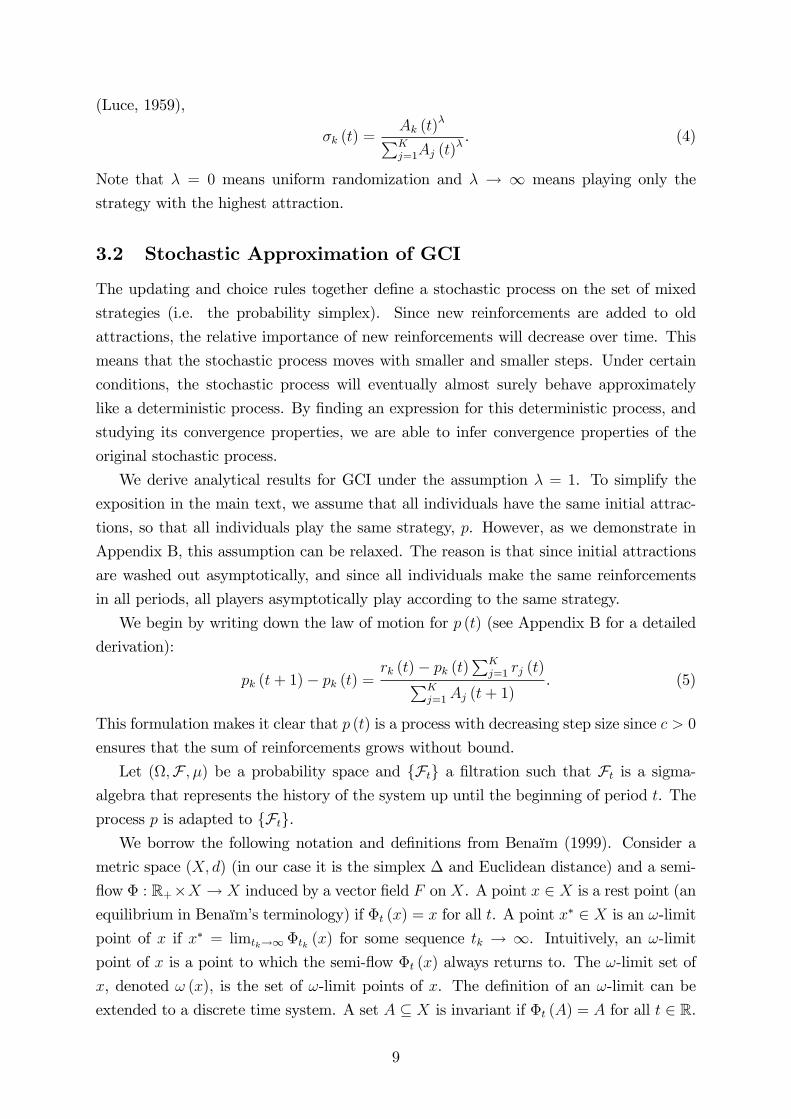
3.2 Stochastic Approximation of GCI
The updating and choice rules together define a stochastic process on the set of mixed
strategies (i.e. the probability simplex). Since new reinforcements are added to old
attractions, the relative importance of new reinforcements will decrease over time. This
means that the stochastic process moves with smaller and smaller steps. Under certain
conditions, the stochastic process will eventually almost surely behave approximately
like a deterministic process. By finding an expression for this deterministic process, and
studying its convergence properties, we are able to infer convergence properties of the
original stochastic process.
We derive analytical results for GCI under the assumption λ = 1. To simplify the
exposition in the main text, we assume that all individuals have the same initial attrac-
tions, so that all individuals play the same strategy, p. However, as we demonstrate in
Appendix B, this assumption can be relaxed. The reason is that since initial attractions
are washed out asymptotically, and since all individuals make the same reinforcements
in all periods, all players asymptotically play according to the same strategy.
We begin by writing down the law of motion for p (t) (see Appendix B for a detailed
derivation):
pk (t+ 1)− pk (t) =rk (t)− pk (t)
∑Kj=1 rj (t)∑K
j=1Aj (t+ 1). (5)
This formulation makes it clear that p (t) is a process with decreasing step size since c > 0
ensures that the sum of reinforcements grows without bound.
Let (Ω,F , µ) be a probability space and Ft a filtration such that Ft is a sigma-algebra that represents the history of the system up until the beginning of period t. The
process p is adapted to Ft.We borrow the following notation and definitions from Benaïm (1999). Consider a
metric space (X, d) (in our case it is the simplex ∆ and Euclidean distance) and a semi-
flow Φ : R+×X → X induced by a vector field F on X. A point x ∈ X is a rest point (an
equilibrium in Benaïm’s terminology) if Φt (x) = x for all t. A point x∗ ∈ X is an ω-limit
point of x if x∗ = limtk→∞Φtk (x) for some sequence tk → ∞. Intuitively, an ω-limitpoint of x is a point to which the semi-flow Φt (x) always returns to. The ω-limit set of
x, denoted ω (x), is the set of ω-limit points of x. The definition of an ω-limit can be
extended to a discrete time system. A set A ⊆ X is invariant if Φt (A) = A for all t ∈ R.
9
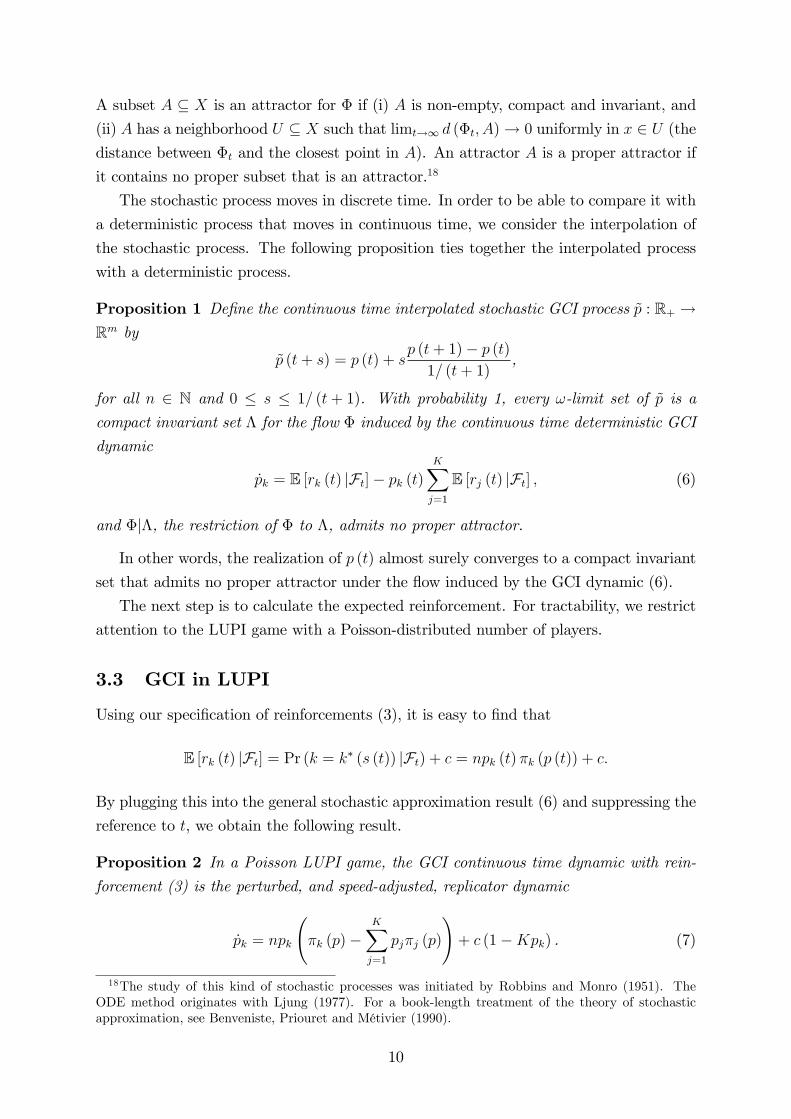
A subset A ⊆ X is an attractor for Φ if (i) A is non-empty, compact and invariant, and
(ii) A has a neighborhood U ⊆ X such that limt→∞ d (Φt, A)→ 0 uniformly in x ∈ U (thedistance between Φt and the closest point in A). An attractor A is a proper attractor if
it contains no proper subset that is an attractor.18
The stochastic process moves in discrete time. In order to be able to compare it with
a deterministic process that moves in continuous time, we consider the interpolation of
the stochastic process. The following proposition ties together the interpolated process
with a deterministic process.
Proposition 1 Define the continuous time interpolated stochastic GCI process p : R+ →Rm by
p (t+ s) = p (t) + sp (t+ 1)− p (t)
1/ (t+ 1),
for all n ∈ N and 0 ≤ s ≤ 1/ (t+ 1). With probability 1, every ω-limit set of p is a
compact invariant set Λ for the flow Φ induced by the continuous time deterministic GCI
dynamic
pk = E [rk (t) |Ft]− pk (t)K∑j=1
E [rj (t) |Ft] , (6)
and Φ|Λ, the restriction of Φ to Λ, admits no proper attractor.
In other words, the realization of p (t) almost surely converges to a compact invariant
set that admits no proper attractor under the flow induced by the GCI dynamic (6).
The next step is to calculate the expected reinforcement. For tractability, we restrict
attention to the LUPI game with a Poisson-distributed number of players.
3.3 GCI in LUPI
Using our specification of reinforcements (3), it is easy to find that
E [rk (t) |Ft] = Pr (k = k∗ (s (t)) |Ft) + c = npk (t) πk (p (t)) + c.
By plugging this into the general stochastic approximation result (6) and suppressing the
reference to t, we obtain the following result.
Proposition 2 In a Poisson LUPI game, the GCI continuous time dynamic with rein-forcement (3) is the perturbed, and speed-adjusted, replicator dynamic
pk = npk
(πk (p)−
K∑j=1
pjπj (p)
)+ c (1−Kpk) . (7)
18The study of this kind of stochastic processes was initiated by Robbins and Monro (1951). TheODE method originates with Ljung (1977). For a book-length treatment of the theory of stochasticapproximation, see Benveniste, Priouret and Métivier (1990).
10
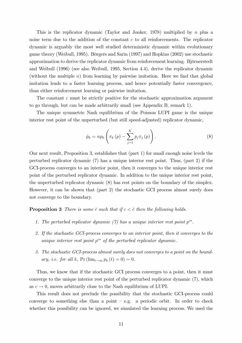
This is the replicator dynamic (Taylor and Jonker, 1978) multiplied by n plus a
noise term due to the addition of the constant c to all reinforcements. The replicator
dynamic is arguably the most well studied deterministic dynamic within evolutionary
game theory (Weibull, 1995). Börgers and Sarin (1997) and Hopkins (2002) use stochastic
approximation to derive the replicator dynamic from reinforcement learning. Björnerstedt
and Weibull (1996) (see also Weibull, 1995, Section 4.4), derive the replicator dynamic
(without the multiple n) from learning by pairwise imitation. Here we find that global
imitation leads to a faster learning process, and hence potentially faster convergence,
than either reinforcement learning or pairwise imitation.
The constant c must be strictly positive for the stochastic approximation argument
to go through, but can be made arbitrarily small (see Appendix B, remark 1).
The unique symmetric Nash equilibrium of the Poisson LUPI game is the unique
interior rest point of the unperturbed (but still speed-adjusted) replicator dynamic,
pk = npk
(πk (p)−
K∑j=1
pjπj (p)
). (8)
Our next result, Proposition 3, establishes that (part 1) for small enough noise levels the
perturbed replicator dynamic (7) has a unique interior rest point. Thus, (part 2) if the
GCI-process converges to an interior point, then it converges to the unique interior rest
point of the perturbed replicator dynamic. In addition to the unique interior rest point,
the unperturbed replicator dynamic (8) has rest points on the boundary of the simplex.
However, it can be shown that (part 2) the stochastic GCI process almost surely does
not converge to the boundary.
Proposition 3 There is some c such that if c < c then the following holds.
1. The perturbed replicator dynamic (7) has a unique interior rest point pc∗.
2. If the stochastic GCI-process converges to an interior point, then it converges to the
unique interior rest point pc∗ of the perturbed replicator dynamic.
3. The stochastic GCI-process almost surely does not converges to a point on the bound-
ary, i.e. for all k, Pr (limt→∞ pk (t) = 0) = 0.
Thus, we know that if the stochastic GCI process converges to a point, then it must
converge to the unique interior rest point of the perturbed replicator dynamic (7), which
as c→ 0, moves arbitrarily close to the Nash equilibrium of LUPI.
This result does not preclude the possibility that the stochastic GCI-process could
converge to something else than a point — e.g. a periodic orbit. In order to check
whether this possibility can be ignored, we simulated the learning process. We used the
11

lab parameters K = 99 and n = 26.9, and randomly drew 100 different initial conditions.
For each initial condition, we ran the process for 10 million rounds. The simulated
distribution is virtually indistinguishable from the equilibrium distribution except for the
numbers 11-14, where some minor deviations occur. This is illustrated in Figure D1 in
Appendix D. It strongly indicates global convergence of the stochastic GCI process in
LUPI.
In Appendix D, we also study the local stability properties of the unique interior
rest point by combining analytical and numerical methods. Analytically, we establish
that local stability under the perturbed dynamic is guaranteed if all the eigenvalues of a
particular matrix are negative. Furthermore, if this holds then the equilibrium p∗ is an
evolutionarily stable strategy. Due to the nonlinearity of payoffs we are only able to check
the eigenvalues with the help of numerical methods, and even for a computer this is only
possibly to do for the parameter values from the laboratory version of LUPI; not for the
parameter values in the field. For the laboratory parameter values we do indeed find that
all eigenvalues are negative. This implies that, p∗ is an evolutionarily stable strategy, and
with positive probability the stochastic GCI-process converges to the unique interior rest
point of the perturbed replicator dynamic, at least for the parameters of the laboratory
LUPI game.19
We conclude this section by noting that the Poisson LUPI game has a special property
that may provide some further intuition for why imitation of winners leads to equilibrium
in LUPI. Let wk be the probability that number k wins the game. From the above, we
know that wk = npkπk. Since it is always possible that no number is chosen uniquely, the
wk’s will not sum up to one, i.e.∑wk < 1. Note that the payoff πk is the probability
that one player wins by playing k while all other players play according to the mixed
strategy p.
Proposition 4 Consider the Poisson LUPI game and suppose that p has full support.There is probability matching, pk = wk/
∑j wj for all k, if and only if p is the symmetric
Nash equilibrium.
This result suggests that players might converge to equilibrium by simply choosing
numbers in proportion to how often those numbers have won in the past.
19The fact that the unique interior Nash equilibrium is an evolutionarily stable strategy may providesome intuition for why we observe convergence. Roughly, one may think of strategies that put more prob-ability on lower numbers than the equilibrium strategy as Hawkish. Likewise one may think of strategiesthat put more probability in higher numbers than the equilibrium strategy, as Dove-like. As in a classicHawk-Dove game the benefit of Hawkish and Dove-like strategies in LUPI is decreasing in the fractionof the population that use Hawkish and Dove-like strategies, respectively. In the Hawk-Dove game thisnegative correlation between fractions and payoffs of strategies pushes adaptive learners towards theunique interior Nash equilibrium and evolutionarily stable strategy. A similar logic is responsible forconvergence in LUPI.
12

3.4 GCI for General Games
To extend the application of the GCI model beyond LUPI, we need to calculate expected
reinforcement more generally. This requires us to make two distinctions. First, imitation
may or may not be responsive to the number of people who play different strategies, so we
distinguish frequency-dependent (FD) and frequency-independent (FI) versions of GCI.
For simplicity, we assume a multiplicative interaction between payoffs and frequencies,
i.e. reinforcement in the frequency-dependent model depends on the total payoff of all
players that picked an action. Second, imitation may be exclusively focused on emulating
the winning action, i.e. the action that obtained the highest payoff, or be responsive
to payoff-differences in a proportional way, so we differentiate between winner—takes-all
imitation (W) and payoff-proportional imitation (P). In total, we propose the following
four members of the GCI family: PFI, PFD, WFD, and WFI.
In Appendix C, we discuss these different versions of GCI in greater detail. In particu-
lar, we show that in LUPI they all coincide with a Poisson distributed number of players.
Furthermore, we show that, in general, it is only the payoff-proportional and frequency-
dependent version (PFD) of GCI that induces the replicator dynamic multiplied by the
expected number of players as its associated continuous time dynamic. PFD can be used
in information environments where there is population-wide information available about
both payoffs and frequencies of different actions. In such settings it generates more rapid
learning than either pairwise imitation or reinforcement learning, as described above.
3.5 Similarity-Based Imitation
Since the strategy set is so large in the LUPI field game, only reinforcing the previous
winning number would result in a learning process that is too slow and too tightly clus-
tered on previous winners. Therefore, we follow Sarin and Vahid (2004) by assuming
that numbers that are similar to the winning number may also be reinforced. We use
the triangular Bartlett similarity function used by Sarin and Vahid (2004). This function
implies that strategies close to previous winners are reinforced and that the magnitude
of reinforcement decreases linearly with distance from the previous winner.
Let W denote the size of the “similarity window”and define the similarity function
ηk (k∗) =max
0, 1− |k
∗−k|W
∑K
i=0 max
0, 1− |k∗−i|W
. (9)
This is depicted in Figure 1 for k∗ = 10 and W = 3. Note that the similarity weights are
normalized so that they sum to one. The stochastic approximation results derived above
hold exactly when W = 1, and we conjecture that they will hold approximately at least
for low values of W > 1.
13

[INSERT FIGURE 1 HERE]
3.6 Empirical Estimation of the Model
The similarity-based learning model presented above has two free parameters: the size of
the similarity window, W , and the precision of the choice function, λ. When estimating
the model, we also need to make assumptions about the choice probabilities in the first
period, as well as the initial sum of attractions.
In our baseline estimations, we fix λ = 1 and determine the best-fitting value of W
by minimizing the squared deviation between predicted choice densities and empirical
densities summed over rounds and choices. We use the empirical frequencies to create
choice probabilities in the first period (“burning in”). Given these probabilities and λ, we
determine A (0) so that equation (4) gives the assumed choice probabilities σk (1). Since
the power choice function is invariant to scaling, the level of attractions is indeterminate.
In our baseline estimations, we scale attractions so that they sum to one, i.e., A0 ≡∑Kk=1Ak (0) = 1. Since the reinforcement factors are scaled to sum to one in each period,
this implies that the first period choice probabilities carry the same weight as each of the
following periods of reinforcement.
The reinforcement factors rk (t) depend on the winning number in t. For the empirical
estimation of the learning model, we use the actual winning numbers.
4 The Field LUPI Game
The field version of LUPI, called Limbo, was introduced by the government-owned Swedish
gambling monopoly Svenska Spel on the 29th of January 2007. We have obtained daily
aggregate choice data from Östling et al. (2011) for the first seven weeks of the game.
This section describes its essential elements; additional details about the game is available
in Östling et al. (2011).
In the Limbo-version of LUPI, K = 99, 999 and each player had to pay 10 SEK
(approximately 1 euro) for each bet. The total number of bets for each player was
restricted to six. The game was played daily. The winner was guaranteed to win at least
100, 000 SEK, but there were also smaller second and third prizes (of 1, 000 SEK and 20
SEK) for being close to the winning number. It was possible for players to let a computer
choose random numbers for them. We cannot disentangle such random choices and they
are therefore included in the data.
Players could access the full distribution of previous choices through the company web
site. However, this data was available in the form of raw text files and it is unlikely that
many players looked at this data. Information about winning numbers as well as some
popular numbers was much more readily available on the web site and in a daily evening
14

TV show. Information about previous winning numbers was also available on posters at
many outlets of the gambling company. See the Online Appendix of Östling et al. (2011)
for further details and examples of the feedback that players received. In sum, the most
commonly encountered feedback was the information about past winning bids.
The theoretical analysis of the LUPI game differs from Limbo in some ways. The tie-
breaking rule is different, but this is unlikely to play a role since the probability that there
is no unique number is very small (it never happened in the field). A second difference
is that players in the field were allowed to bet on up to six numbers. Third, we do not
take the second and third prizes present in the field version into account. In addition,
we assume that the number of players is Poisson distributed, whereas the variance in the
number of players is too large to be consistent with this assumption. Finally, we have
(implicitly) assumed that players only had information about previous winning numbers,
whereas more detailed information was available.
These differences between Limbo and the game analyzed theoretically are an im-
portant motivation for also studying the data from Östling et al’s (2011) laboratory
experiment, which matches the theoretical assumptions more closely.
4.1 Descriptive Statistics
Table 1 reports weekly summary statistics for the game. The last column displays the
corresponding statistics that would result from play according to the symmetric Poisson-
Nash equilibrium.20 In the first week behavior is quite far from equilibrium: the average
chosen number is far above what it should be in equilibrium; and both the median chosen
number and the average winning number is below what it should be in equilibrium.
However, behavior changes rapidly over time. Towards the end of the period the data is
quite closely aligned with the equilibrium prediction, as discussed at length by Östling
et al. (2011). For example, both average winning numbers and the average numbers
played in later rounds are similar to the equilibrium prediction. (Note that the probability
matching result of Proposition 4 implies that, in equilibrium, the average winning number
is the same as the average number played.) The median chosen number is much lower
than the average number —which is due to some players playing very high numbers —
but the difference between the average and the median decreases over time. The full
empirical distribution, displayed in figure 5 below, gives a similar impression.
20An alternative theoretical benchmark is quantal response equilibrium (QRE). However, Östling et al.(2011) show that QRE is unlikely to fit the data any better than the Poisson-Nash equilibrium.
15
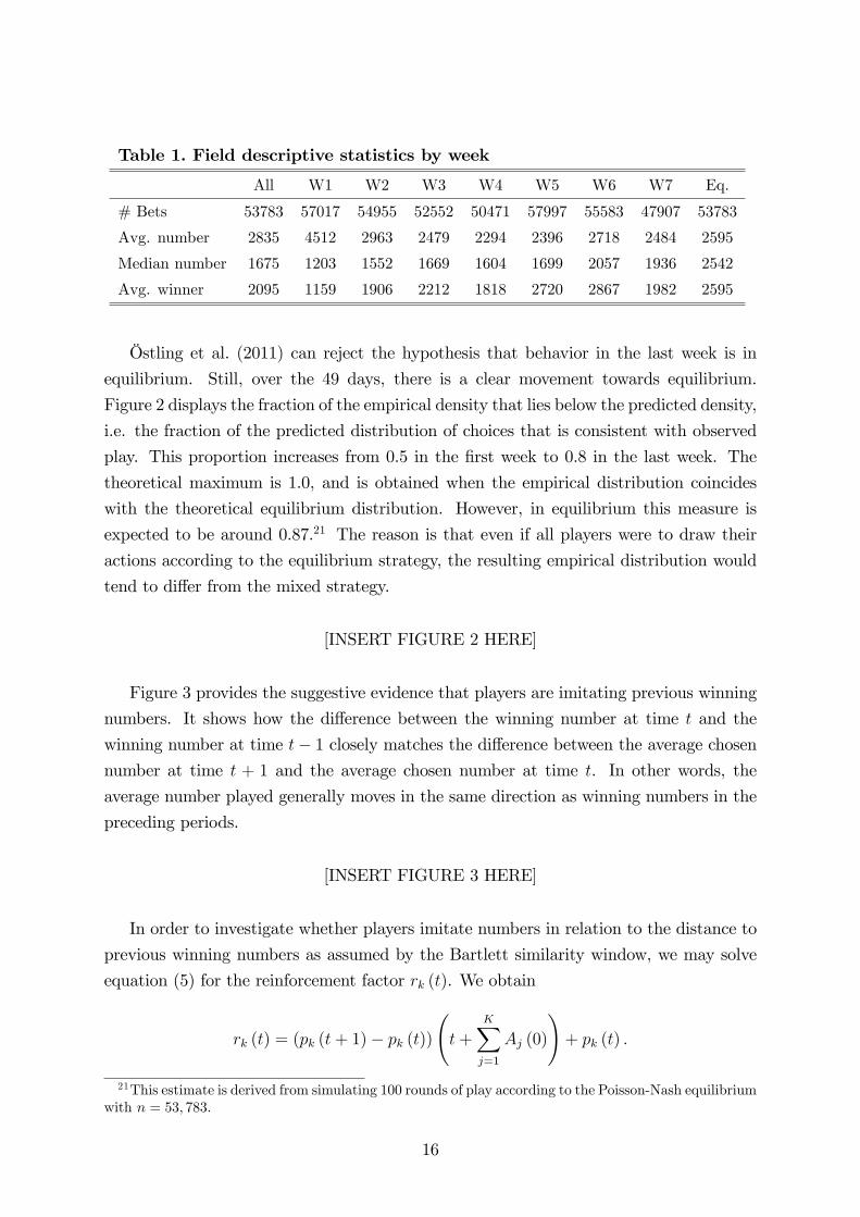
Table 1. Field descriptive statistics by week
All W1 W2 W3 W4 W5 W6 W7 Eq.
# Bets 53783 57017 54955 52552 50471 57997 55583 47907 53783
Avg. number 2835 4512 2963 2479 2294 2396 2718 2484 2595
Median number 1675 1203 1552 1669 1604 1699 2057 1936 2542
Avg. winner 2095 1159 1906 2212 1818 2720 2867 1982 2595
Östling et al. (2011) can reject the hypothesis that behavior in the last week is in
equilibrium. Still, over the 49 days, there is a clear movement towards equilibrium.
Figure 2 displays the fraction of the empirical density that lies below the predicted density,
i.e. the fraction of the predicted distribution of choices that is consistent with observed
play. This proportion increases from 0.5 in the first week to 0.8 in the last week. The
theoretical maximum is 1.0, and is obtained when the empirical distribution coincides
with the theoretical equilibrium distribution. However, in equilibrium this measure is
expected to be around 0.87.21 The reason is that even if all players were to draw their
actions according to the equilibrium strategy, the resulting empirical distribution would
tend to differ from the mixed strategy.
[INSERT FIGURE 2 HERE]
Figure 3 provides the suggestive evidence that players are imitating previous winning
numbers. It shows how the difference between the winning number at time t and the
winning number at time t− 1 closely matches the difference between the average chosen
number at time t + 1 and the average chosen number at time t. In other words, the
average number played generally moves in the same direction as winning numbers in the
preceding periods.
[INSERT FIGURE 3 HERE]
In order to investigate whether players imitate numbers in relation to the distance to
previous winning numbers as assumed by the Bartlett similarity window, we may solve
equation (5) for the reinforcement factor rk (t). We obtain
rk (t) = (pk (t+ 1)− pk (t))
(t+
K∑j=1
Aj (0)
)+ pk (t) .
21This estimate is derived from simulating 100 rounds of play according to the Poisson-Nash equilibriumwith n = 53, 783.
16
In our baseline estimations, we assume that the initial attractions sum to one. Under the
assumption that someone wins in every round (which is indeed the case in the field), this
implies that an empirical estimate of the reinforcement of number k in period t can be
obtained by calculating
rk (t) = [pk (t+ 1)− pk (t)] (t+ 1) + pk (t) ,
where pk (t) is the empirical frequency with which number k is played in t. Note that
this estimation strategy does not assume that reinforcement factors are similarity-based,
only that attractions accumulate according to the updating rule and reinforcements sum
to one.
Figure 4 shows the estimated reinforcement factors close to the winning number,
averaged over days 2 to 49. The reinforcement factor for the winning number is excluded
in order to enhance the readability of the figure (the estimated average reinforcement
for the previous winning number is about 0.007). The black line in Figure 4 shows a
moving average (over 201 numbers) of the reinforcement factors. Note that the estimated
reinforcement factors are symmetric around the winning number and that they could be
quite closely approximated by a Bartlett similarity window of about 1000. The variance
of reinforcement factors is larger for numbers far below the winning number. This is
due to average reinforcement being calculated based on data from relatively few periods
because the winning number is often below 1000.
[INSERT FIGURE 4 HERE]
4.2 Estimation Results
In the baseline estimation, we keep λ fixed and find the best-fitting size of the Bartlett
similarity window, W , by minimizing the sum of squared deviations over all window sizes
W = 500, 501, ..., 2500.22 (We also verified that smaller/larger windows did not improvethe fit.) In our baseline estimation, the best-fitting window is 1999. This implies that
3996 numbers in addition to the winning number are reinforced (as long as the winning
number is above 1998). The sum of squared deviations (SSD) between predicted and
empirical frequencies is 0.0044. This can be compared with a value of 0.0107 for the
Poisson-Nash equilibrium prediction.
Figure 5 displays the predicted densities of the learning model for numbers up to 6000
along with the data and equilibrium from each day from the second day and onwards. To
make the figures readable, the data has been smoothed using moving averages (over 201
22The equilibrium prediction is numerically zero for most numbers and the likelihood of the equilibriumprediction will therefore always be zero. Since we want to compare the fit of the estimated learning modelwith equilibrium, we focus on the sum of squared deviations throughout the paper.
17
numbers). The vertical dotted lines show the winning number on the previous day. The
main feature of learning is that the frequency of very low numbers shrinks and the gap
between the predicted frequency of numbers between 2000 and 5000 is gradually filled in.
[INSERT FIGURE 5 HERE]
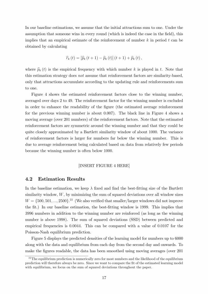
It may appear surprising that the estimated window size is so much larger than what
is suggested by the estimated reinforcements in Figure 4. However, Figure 4 only shows
changes close to the winning number, whereas the learning model also needs to explain
the “baseline” level of choices. If we restrict the similarity window to be 1000, then
the sum of squared deviations is 0.0046, i.e. only a slightly worse fit. The estimated
window size is also sensitive to the assumption about initial choice probabilities and
attractions. To see this, Table 2 shows that the best-fitting window size is smaller if the
initial choice probabilities are uniform, but it is also smaller the more weight is given to
initial attractions.23
Table 2. Estimation of learning model for the field
A0= 0.25 A0= 0.5 A0= 1 A0= 2 A0= 4
W SSD W SSD W SSD W SSD W SSD
Actual 2177 0.0057 2117 0.0051 1999 0.0044 1369 0.0039 1190 0.0042
Uniform 2093 0.0083 1978 0.0083 1392 0.0083 1318 0.0084 1179 0.0086
Finally, we can also estimate the model by fitting bothW and λ. To do this, we letW
vary from 100 and 2500 and determine the best-fitting value of λ through interval search
for each window size (we let λ vary between 0.005 and 2). The best-fitting parameters
are W = 1310 and λ = 0.81. The sum of squared deviations is 0.0043, so letting λ vary
does not seem to improve the fit of the learning model to any particular extent. If we
restrict W = 1000, then the estimated λ is 0.78 and the sum of squared deviations is
0.0043.
5 The Laboratory LUPI Game
The field LUPI game does not exactly match the theoretical assumptions and therefore
we also analyze the laboratory data from Östling et al. (2011) that follows the theory
23We have also estimated the model with a decay factor δ < 1 so that attractions are updated accordingto Ak (t+ 1) = δAk (t) + rk (t). This resulted in a poorer fit and δ seems to play a similar role as A0:the smaller is δ, the poorer is the fit and the larger is the estimated window size.
18

much more closely. Their experiment consisted of 49 rounds in each session and the prize
to the winner in each round was $7. The strategy space was also scaled down so that
K = 99. The number of players in each round was drawn from a distribution with mean
26.9.24 In the laboratory, each player was allowed to choose only one number, they could
not use a random number generator (as in the field game), there was only one prize per
round, and if there was no unique number, nobody won. Crucially, the only feedback
that players received after each round was the winning number.
At the beginning of each session, the experimenter first explained the rules of the
LUPI game. The instructions were based on a version of the lottery form for the field
game translated from Swedish into English (see Östling et al., 2011).
When all subjects had submitted their chosen numbers, the lowest unique positive
integer was determined. If there was a lowest unique positive integer, the winner earned
$7; if no number was unique, no subject won. Each subject was privately informed,
immediately after each round, what the winning number was, whether they had won
that particular round, and their payoff so far during the experiment. This procedure was
repeated 49 times, with no practice rounds. All sessions lasted for less than an hour, and
subjects received a show-up fee of $8 or $13 in addition to earnings from the experiment
(which averaged $8.60). The experiments were conducted at the California Social Science
Experimental Laboratory (CASSEL) at University of California Los Angeles in 2007 and
2009.
A more detailed description of the experiment can be found in Östling et al. (2011).
5.1 Descriptive Statistics
We only focus on the choices from incentivized subjects that were selected to actively
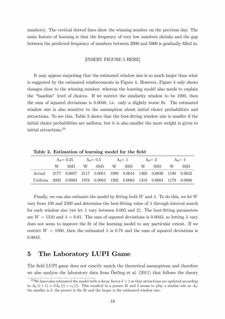
participate in a round.25 Table 3 shows some descriptive statistics for the participating
subjects in the laboratory experiment. As in the field, some players in the first rounds
tend to pick very high numbers (above 20) but the percentage shrinks to approximately
1 percent after the first seven rounds. Both the average and the median number chosen
corresponds closely to the equilibrium after the first seven rounds. The average winning
numbers are too high compared to equilibrium play, which is consistent with players
24In three of the four sessions, subjects were told the mean number of players, and that the numbervaried from round to round, but did not know the distribution (in order to match the field situation inwhich players were very unlikely to know the total number playing each day). Due to a technical error,in these three sessions, the variance was lower than the Poisson variance (7.2 to 8.6 rather than 26.9).However, this mistake is likely to have little effect on behavior because subjects did not know the totalnumber of players in each round. In the last session, the number of players in each round was drawnfrom a Poisson distribution with mean 26.9 and the subjects were informed about this.25At the beginning of each round, subjects were informed whether they would actively participate in
the current round (i.e., if they had a chance to win). They were required to submit a number in eachround, even if they were not selected to participate, and always received information about the winningnumber.
19
picking very low numbers too often, creating non-uniqueness among those numbers so
that unique numbers are unusually high. The overwhelming impression from Table 3
is that convergence (close) to equilibrium is very rapid despite receiving feedback only
about the winning number.
Table 3. Laboratory descriptive statistics
All 1-7 8-14 15-21 22-28 29-35 36-42 43-49 Eq.
Avg. number 5.96 8.56 5.24 5.45 5.57 5.45 5.59 5.84 5.22
Median number 4.65 6.14 4.00 4.57 4.14 4.29 4.43 5.00 5.00
Avg. winner 5.63 8.00 5.00 5.22 6.00 5.19 5.81 4.12 5.22
Below 20 (%) 98.02 93.94 99.10 98.45 98.60 98.85 98.79 98.42 100.00
Figure 6 shows that there is a movement towards equilibrium as measured by the
proportion of the empirical density below the predicted density. The dashed lines in
Figure 6 show fitted linear trends, which are upward-sloping in all sessions. In addition,
towards the end of the period, the measure is very close to what is expected if players
played equilibrium —in equilibrium this statistic would be 0.74.26
[INSERT FIGURE 6 HERE]
Östling et al. (2011) report the result from a post-experimental questionnaire. A
notable finding from their analysis was that several subjects said that they responded to
previous winning numbers. To investigate whether this is reflected in subjects’choices,
Table 4 displays the results from an OLS regression with changes in average guesses as
the dependent variable, and lagged differences between winning numbers as independent
variables. Lagged changes in winning numbers have a clear relationship with average
choices. Comparing the first 14 rounds with the last 14 rounds, the estimated coeffi cients
are very similar, but the explanatory power of past winning numbers is much higher in
the early rounds (R2 is 0.026 in the first 14 rounds and 0.003 in the last 14 rounds).
The fact that the relationship is weaker in later rounds is consistent with the GCI model
since the decreasing step size implies that the influence of winning numbers grows smaller
over time. Figure E2 in Appendix E illustrates the co-movement of average guesses and
previous winning numbers graphically.
26As a further illustration of convergence to equilibrium, Figure E1 in Appendix E displays the distri-bution of chosen and winning number in all session from period 25 and onwards. Recall from Proposition4 that, in equilibrium, the choice probabilities should coincide with the probability that each numberwins, and, as can be seen from Figure E1, the correspondence is quite close.
20
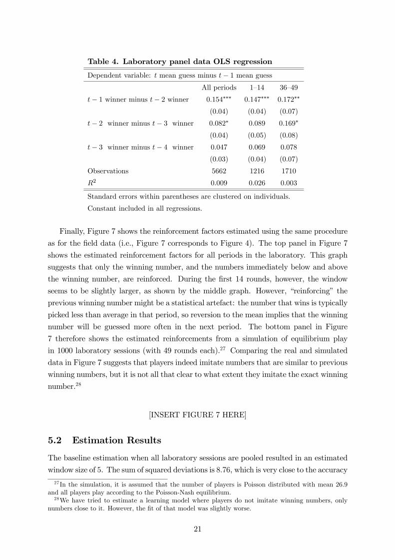
Table 4. Laboratory panel data OLS regression
Dependent variable: t mean guess minus t− 1 mean guessAll periods 1—14 36—49
t− 1 winner minus t− 2 winner 0.154∗∗∗ 0.147∗∗∗ 0.172∗∗
(0.04) (0.04) (0.07)
t− 2 winner minus t− 3 winner 0.082∗ 0.089 0.169∗
(0.04) (0.05) (0.08)
t− 3 winner minus t− 4 winner 0.047 0.069 0.078
(0.03) (0.04) (0.07)
Observations 5662 1216 1710
R2 0.009 0.026 0.003
Standard errors within parentheses are clustered on individuals.
Constant included in all regressions.
Finally, Figure 7 shows the reinforcement factors estimated using the same procedure
as for the field data (i.e., Figure 7 corresponds to Figure 4). The top panel in Figure 7
shows the estimated reinforcement factors for all periods in the laboratory. This graph
suggests that only the winning number, and the numbers immediately below and above
the winning number, are reinforced. During the first 14 rounds, however, the window
seems to be slightly larger, as shown by the middle graph. However, “reinforcing” the
previous winning number might be a statistical artefact: the number that wins is typically
picked less than average in that period, so reversion to the mean implies that the winning
number will be guessed more often in the next period. The bottom panel in Figure
7 therefore shows the estimated reinforcements from a simulation of equilibrium play
in 1000 laboratory sessions (with 49 rounds each).27 Comparing the real and simulated
data in Figure 7 suggests that players indeed imitate numbers that are similar to previous
winning numbers, but it is not all that clear to what extent they imitate the exact winning
number.28
[INSERT FIGURE 7 HERE]
5.2 Estimation Results
The baseline estimation when all laboratory sessions are pooled resulted in an estimated
window size of 5. The sum of squared deviations is 8.76, which is very close to the accuracy
27In the simulation, it is assumed that the number of players is Poisson distributed with mean 26.9and all players play according to the Poisson-Nash equilibrium.28We have tried to estimate a learning model where players do not imitate winning numbers, only
numbers close to it. However, the fit of that model was slightly worse.
21

of the equilibrium prediction (8.79). As discussed in the previous section, players in the
laboratory seem to learn to play the game more quickly than in the field, so there is less
learning to be explained by the learning model. The difference between the learning model
and equilibrium is consequently larger in early rounds. If only the seven first rounds are
used to estimate the learning model, the best-fitting window size is 6 and the sum of
squared deviations 1.19, which can be compared to the equilibrium fit of 1.52. However,
since the learning model uses actual first-period choice probabilities, this comparison is
unfair. If we instead base the initial choice probabilities of the learning model on the
equilibrium prediction, the learning model improves much less on equilibrium (1.45 vs.
1.52 for the first seven rounds).
Table 5 shows the estimated window sizes for different initial choice probabilities and
weights on initial attractions. The estimated window size is typically smaller when the
initial attractions are scaled up. It is clear that our model works best in the initial rounds
of play. This is only to be expected since this is when most of the learning takes place
in the lab. Figures E3 to E6 in Appendix E therefore show the prediction of the learning
model along with the data and equilibrium prediction for rounds 2-6 for each session
separately.
Table 5. Estimation of learning model for LUPI in the laboratory
A0= 0.25 A0 = 0.5 A0= 1 A0= 2 A0= 4 Eq.
W SSD W SSD W SSD W SSD W SSD SSD
Period 1-7
Actual 8 1.19 8 1.18 6 1.19 6 1.25 6 1.38
Uniform 8 1.49 8 1.51 6 1.57 6 1.72 6 1.97
Equilibrium 8 1.46 8 1.46 8 1.45 8 1.45 6 1.45 1.52
Period 1-14
Actual 6 2.83 6 2.80 6 2.80 5 2.87 5 3.07
Uniform 6 3.14 6 3.15 6 3.24 5 3.44 4 3.84
Equilibrium 7 3.11 6 3.09 6 3.05 6 3.02 5 2.99 3.02
Period 1-49
Actual 5 8.87 5 8.80 5 8.76 4 8.78 4 8.99
Uniform 5 9.20 5 9.19 5 9.28 4 9.50 4 10.06
Equilibrium 5 9.16 5 9.09 5 9.01 4 8.92 4 8.81 8.79
Estimated window sizes (W ) and sum of squared deviations (SSD) between data
and model when λ = 1. Initial attractions for learning model are determined by
actual choices, a uniform distribution or the Poisson-Nash equilibrium.
22

Table 6 reports the results when we allow λ to vary and restrict the attention to
the first 7 rounds. In this estimation, we calculate the best-fitting lambda for window
sizes W = 1, 2, 3, .., 15. Allowing λ to vary slightly improves the fit, but not to anyparticularly large extent. It can also be noted that W does not vary systematically with
the scale of initial attractions. This might be due to diffi culties in estimating the model
with two parameters. The sum of squared deviations is relatively flat with respect to W
and λ when both parameters increase proportionally. A higher window size W combined
with higher response sensitivity λ generates a very similar sum of squared deviations
(since a higher W is generating a wider spread of responses and a higher λ is tightening
the response).
Table 6. Estimation of learning model round 1-7
A0=0.5 A0=1 A0=2 Eq.
W λ SSD W λ SSD W λ SSD SSD
Actual 8 1.16 1.17 8 1.33 1.17 6 1.35 1.21
Uniform 9 1.27 1.48 11 1.67 1.49 11 1.97 1.49
Equilibrium 8 0.98 1.46 8 1.00 1.45 8 0.99 1.45 1.52
Estimated window sizes (W ), precision parameter λ and sum of squared
deviations (SSD) between data and model. Initial attractions are determined
by actual choices, a uniform distribution or the Poisson-Nash equilibrium.
6 Out-Of-Sample Explanatory Power
Similarity-based GCI seems to be able to capture how players in both the field and the
laboratory learn to play the LUPI game. However, the learning model was developed after
observing Östling et al’s (2011) LUPI data, which might raise worries that the model is
only suited to explain learning in this particular game. Therefore, we decided to conduct
new experiments with three other games. We made no changes to the similarity-based
GCI model after observing the results from these additional experiments.
We selected the games based on the following three criteria. First, we only considered
symmetric games with large, ordered strategy sets so that similarity-based learning makes
sense. Second, we selected games with relatively complex rules so that it would not
be transparent to calculate best responses. Finally, since we did not want to try to
discriminate between the four different members of the GCI family, we only considered
games where at most one player wins a fixed positive payoff and the remaining players
earn nothing.
23

In all three games, there is a fixed number of players who choose integers from 1 to K
simultaneously. There is at most one winner who earns a positive payoff, while all others
earn 0. We call the first of our three games the second lowest unique positive integer
(SLUPI) game, i.e. the player that picks the second lowest unique number wins. If there
is no winner, no player gets anything. SLUPI does not have a symmetric mixed strategy
equilibrium, but the game has K symmetric pure strategy equilibria, in which all players
choose the same number.29
The second game is the center-most unique positive integer (CUPI) game. In this
game, the uniquely chosen number that is closest to 50 wins. In case there are two
uniquely chosen numbers with the same distance to the center, the higher of the two
numbers wins. The CUPI game is simply the LUPI game with a re-shuffl ed strategy
space. If the number of players is Poisson distributed, it is straightforward to prove that
Proposition 2 applies to both CUPI and SLUPI, i.e. that the GCI learning model induces
the perturbed replicator dynamic.
The third game is a variant of the beauty contest (BC) game (Nagel, 1995, Ho,
Camerer and Weigelt, 1998). In this game, the player that picks an integer closest to a
target wins and the remaining players earn nothing. If several players’guesses are closest
to the target, one randomly chosen player wins. The target is p times the median guess
plus a constant m, and we therefore call this game pmBC. The unique Nash equilibrium
of this game is that all players choose the integer closest to m/ (1− p). In our laboratoryexperiment, p = 0.3 and m = 5 so that the unique Nash equilibrium is that all players
choose number 7.
6.1 Experimental Design
Experiments were run at the Taiwan Social Sciences Experimental Laboratory (TASSEL),
National Taiwan University in Taipei, Taiwan, during June 23-27, 2014. We conducted
three sessions with 29 or 31 players in each session.30 In each session, all subjects actively
participated in 20 rounds of each of the three games described above. The order of the
games varied across sessions: CUPI-pmBC-SLUPI in the first session (June 23), pmBC-
CUPI-SLUPI in the second (June 25) and SLUPI-pmBC-CUPI in the third session (June
27). The prize to the winner in each round was NT$200 (approximately US$7 at the
time of the experiment). Each subject was informed, immediately after each round,
what the winning number was (in case there was a winning number), whether they had
29To see why there is no symmetric mixed strategy equilibrium, note that the lowest number in thesupport of such an equilibrium is guaranteed not to win. For the expected payoff to be the same for allnumbers in the equilibrium support, higher numbers in the equilibrium support must be guaranteed notto win. This can only happen if the equilibrium consists of two numbers, but in that case the expectedpayoff from playing some other number would be positive.30Prior to these three sessions we also ran one session where only 14 subjects showed up and we
therefore omit the results from this session.
24

won in that particular round, and their payoff so far during the experiment. There
were no practice rounds. All sessions lasted for less than 125 minutes, and the subjects
received a show-up fee of NT$100 (approximately US$3.5) in addition to earnings from the
experiment (which averaged NT$380.22, ranging from NT$0 to NT$1200). Experimental
instructions translated from Chinese are available in Appendix F. The experiments were
conducted using the experimental software zTree 3.4.2 (Fischbacher, 2007) and subjects
were recruited using the TASSEL website.
6.2 Descriptive Statistics
Figure 8 shows how subjects played in the first and last five rounds in the three different
games. The black lines show the mixed Poisson-Nash equilibrium of the CUPI game
(with 30 players). Since there is no obvious theoretical benchmark for the SLUPI game,
we instead simulate 20 rounds of the similarity-based GCI 100,000 times and show the
average prediction for the last round. In this simulation, we set λ = 1 and use the best-
fitting window size for the first 20 rounds of the LUPI laboratory experiment (W = 5).
The initial attractions were uniform.
[INSERT FIGURE 8 HERE]
It is clear from Figure 8 that players learn to play close to the theoretical benchmark
in all three games. The learning pattern is particularly striking in the pmBC game: in
the first period, 9% play the equilibrium strategy, which increases to 62% in round 5 and
95% in round 10. In the CUPI game, subjects primarily learn not to play 50 so much —
in the first round 26 percent of all subjects play 50 —and there are fewer guesses far from
50. In the SLUPI game, it is less clear how behavior changes over time, but it is clear
that there are fewer very high choices in the later periods.
To investigate whether subjects adjust their choices in response to past winners, we
run the same kind of regression as we did for the LUPI lab data: OLS regressions with
changes in average guesses as the dependent variable, and lagged differences between
winning numbers as independent variables. In LUPI, pmBC and SLUPI, it is clear that
the prediction of similarity-based GCI is that lagged differences between winning numbers
should be positively related to differences in average guesses. In CUPI, however, it is
possible that players instead imitate numbers that are similar in terms of distance to
the center rather than similar in terms of actual numbers. Therefore, we also report the
results after transforming the strategy space. In this transformation, we re-order the
strategy space by distance to the center so that 50 is mapped to 1, 51 to 2, 49 to 3, 52
to 4 and so on. The regression results are reported in Table 7.
25

Table 7. Panel data OLS regression in SLUPI, pmBC, and CUPI
Dependent variable: t mean guess minus t− 1 mean guessSLUPI pmBC CUPI CUPI (trans.)
1—20 1—5 1—20 1—5 1—20 1—5 1—20 1—5
Change in t—1 0.136∗∗∗ 0.259∗∗∗ 1.761 1.975∗∗∗ -0.022 -0.079 0.027 0.150∗∗
(0.04) (0.06) (1.91) (0.49) (0.01) (0.07) (0.01) (0.06)
Change in t—2 -0.007 -0.469 -0.009 0.024
(0.01) (0.75) (0.01) (0.01)
Change in t—3 -0.007 - -0.020 0.031
(0.01) - (0.02) (0.02)
Observations 1456 273 1547 273 1456 273 1456 273
R2 0.112 0.040 0.001 0.066 0.004 0.009 0.008 0.051
Standard errors within parentheses are clustered at the individual level. Constant included in
all regressions. The last regression for periods 1—20 in pmBC is omitted due to collinearity.
In SLUPI and pmBC, it is clear that guesses move in the same direction as the
winning number in the previous round during the first five rounds. After the initial five
rounds, this tendency is less clear, especially in the pmBC game where players learn
to play equilibrium very quickly. In the CUPI, subjects seem to imitate based on the
transformed strategy set rather than actual numbers. In the remainder of the paper, we
therefore report CUPI results with the transformed strategy space. Again, the tendency
to imitate is strongest during the first five rounds. It is primarily during these first periods
that we should expect our model to predict well, because learning slows down after the
initial periods. The effect of winning numbers on chosen numbers in pmBC, CUPI and
SLUPI is illustrated in Figure E7 in Appendix E.
We also estimate the reinforcement factors following the same procedure as in LUPI.
The result when all periods are included is shown in Figure 9. Since there is most clear
evidence of imitation in early rounds, Figure E8 in Appendix E reports the corresponding
estimation when restricting the attention to periods 1-5 only. Figure 9 indicates that
there is a triangular singularity window in both SLUPI and CUPI. As Figure E8 reveals,
however, this is less clear in early rounds —players seem to avoid imitating the exact
winning number from the previous round. In pmBC, players are predominantly playing
the previous winning number which is due to the fact that most players always play
equilibrium after the fifth round. When restricting the attention to the first five periods,
estimated reinforcement has a triangular shape, although it is clear that players primarily
imitate the winning number and numbers below the winning number.
26

[INSERT FIGURE 9 HERE]
6.3 Estimation Results
The results in the previous section suggest that the similarity-based GCI model might be
able to explain the learning pattern observed in the data. To verify this, we set λ = 1 and
fixed the window size at W = 5, which was the best-fitting window size for the first 20
periods in the laboratory LUPI game. As in our baseline estimation for the LUPI game,
we burn in attractions using first-period choices and set the sum of initial attractions to
1. The results are displayed in Table 8. We also separately report the best-fitting window
for each of the three games. As a comparison, we report the GCI model without similarity
(i.e. W = 1) as well as the fit of the equilibrium prediction for CUPI and pmBC.
Table 8. Estimation results for SLUPI, pmBC and CUPI
LUPI SLUPI pmBC CUPI
W SSD W SSD W SSD W SSD
GCI with LUPI window 5 4.08 5 2.74 5 31.16 5 2.57
GCI with best-fitting window 5 4.08 4 2.71 1 5.54 6 2.56
GCI without window 1 12.99 1 8.07 1 5.54 1 8.03
Equilibrium 4.37 9.23 2.96
Estimated window sizes (W ) and sum of squared deviations (SSD) between data and
similarity-based GCI learning model with λ = 1.
Table 8 shows that the window size estimated using the LUPI data is close to the best-
fitting window size in both SLUPI and CUPI. In both these games, the fit is considerably
poorer without the similarity-based window, indicating that similarity is important to
explain the speed of learning in these games. The learning model seems to improve a
little over the equilibrium prediction for the CUPI game, but not to any large extent. In
the pmBC game, however, the window estimated using the LUPI data provides a poor
fit and the best-fitting window is 1. This is primarily due to so many players playing
the equilibrium number in later rounds. If the model is estimated using only the first
five periods, the window size from LUPI gives a similar fit to the best-fitting window
size.31 Comparing the SSD scores across games, it can be noted that our learning model
performs no worse in the new games SLUPI and CUPI than in LUPI, the game for which
it was initially created.31Estimating the data from the pmBC game using period 1-5 data only, W = 5 results in sum of
squared deviations of 1.79, whereas the best-fitting window is 3 and gives squared deviations of 1.61.The sum of squared deviations from the equilibrium prediction is 8.59.
27

6.4 Alternative Learning Models
As discussed in the introduction, most standard learning models are unable to explain
behavior in the LUPI game because they presume the existence of feedback that is not
available to our subjects. In this way, we can rule out fictitious play (e.g. Fudenberg and
Levine, 1998), experiences weighted attraction (EWA) learning (Camerer and Ho, 1999
and Ho et al., 2007), action sampling learning and impulse matching learning (Chmura
et al., 2012), and myopic best response (Cournot) dynamic.32 These observations also
apply to SLUPI and CUPI, whereas there are several possible learning models that can
explain learning in the pmBC.
Table 9. Imitation vs Reinforcement Learning
LUPI SLUPI pmBC CUPI
W SSD W SSD W SSD W SSD
Period 1-5
GCI 7 0.81 6 0.55 3 1.61 7 0.58
Reinforcement learning 3 1.44 3 0.94 1 2.67 4 0.82
Period 1-20
GCI 5 4.08 4 2.71 1 5.54 6 2.56
Reinforcement learning 3 6.90 1 5.25 1 28.41 2 4.23
Estimated window sizes (W ) and sum of squared deviations (SSD)
for reinforcement learning and similarity-based GCI learning model.
The precision parameter λ is set to 1 for both learning models.
Learning based on reinforcement of chosen actions is consistent with the feedback
that our subjects receive in all games we study. However, reinforcement learning is too
slow to explain learning in the field game, because only 49 players win and only these
players would change their behavior. As shown by Sarin and Vahid (2004), reinforcement
learning is quicker if players update strategies that are similar to previous successful
strategies. To see whether similarity-based reinforcement learning can explain behavior
in the laboratory, we compare similarity-based GCI with similarity-based reinforcement
learning. We use the reinforcement learning model of Roth and Erev (1995) since this
model is structurally very similar to GCI —the only difference is that in reinforcement
learning only actions that one has taken oneself are reinforced. Table 9 shows the fit
of the similarity-based GCI model together with the fit of similarity-based reinforcement
32In Appendix A, we argue that more general forms of Bayesian learning are unable to explain theobserved behavior, unless very specific assumptions are made. We also estimate a fictitious play modelusing the field data and show that it fits more poorly than imitation learning.
28
learning. It is clear that GCI results in a better fit than reinforcement learning both when
estimating the model using all data and the first five periods. Table 9 also shows that
during the first five rounds, before behavior has settled down, both GCI and reinforcement
learning fit better with a similarity window —the only exception is the pmBC when data
from all periods is used.
7 Concluding Remarks
This paper utilizes a unique opportunity to study learning and evolutionary game theory
in the field. The rules of the game are clear and we can be relatively confident that
participants strive to maximize the expected payoff, rather than being motivated by social
preferences. Moreover, the game is novel and the equilibrium is diffi cult to compute,
thereby forcing subjects to rely on learning heuristics. In addition, the fact that the
number of participants is so large makes the field LUPI game a suitable testing ground
for evolutionary game theory.
In order to explain the rapid movement toward equilibrium in the field LUPI game,
we develop a new similarity-based imitation learning model and show that it can explain
the most important features of the data. The same model can also explain learning in
the LUPI game played in the laboratory. As a true out-of-sample test of our model, we
conduct an experiment with three additional games and show that our learning model
can explain rapid learning in these games too. Two ingredients of our proposed learning
model merit particular attention in future research. Both ingredients were introduced in
order to successfully explain the speed of learning we see in the data.
The first ingredient is that imitation is global, i.e. players imitate all players’strategy
choices in proportion to the payoff they received. This is crucial for explaining rapid
learning in the LUPI game —pairwise imitation or reinforcement learning based only on
own experience would imply too slow learning. In the LUPI game, global imitation is
equivalent to only imitating the best strategy choice. This seems to be a type of learning
that it would be interesting to study more generally, in particular since many settings
naturally provide a disproportionate amount of information about successful players.
The second ingredient of our learning model is that players imitate numbers that are
“similar” to winning numbers. Similarity in the model is operationalized as a triangu-
lar window around the previous winning number, but our results reveal that people’s
similarity-based reasoning appears to be slightly more sophisticated. For example, the
estimated window sizes do not seem to be proportional to the size of the strategy space
(the similarity window relative to the size of the strategy space is much larger in the
laboratory than in the field). Furthermore, in the laboratory data, there is some indica-
tion that players avoid exactly the winning number in the unique positive integer games,
whereas the similarity window is asymmetric in the beauty contest game. Another sign of
29

more sophisticated similarity-based reasoning is that players in one of the games imitate
numbers based on strategic similarity rather than number similarity.
References
Alos-Ferrer, C. (2004), ‘Cournot versus walras in dynamic oligopolies with memory’,
International Journal of Industrial Organization 22(2), 193—217.
Apesteguia, J., Huck, S. and Oechssler, J. (2007), ‘Imitation—theory and experimental
evidence’, Journal of Economic Theory 136, 217—235.
Armstrong, M. and Huck, S. (2010), ‘Behavioral economics as applied to firms’, Compe-
tition Policy International 6(1), 3—45.
Arthur, W. B. (1993), ‘On designing economic agents that behave like human agents’,
Journal of Evolutionary Economics 3(1), 1—22.
Beggs, A. (2005), ‘On the convergence of reinforcement learning’, Journal of Economic
Theory 122(1), 1—36.
Benaïm, M. (1999), Dynamics of stochastic approximation algorithms, in J. Azéma,
M. Émery, M. Ledoux and M. Yor, eds, ‘Séminaire de Probabilités XXXIII’, Vol. 1709
of Lecture Notes in Mathematics, Springer-Verlag, Berlin/Heidelberg, pp. 1—68.
Benaïm, M. and Weibull, J. W. (2003), ‘Deterministic approximation of stochastic evo-
lution in games’, Econometrica 71(3), 873—903.
Benveniste, A., Priouret, P. and Métivier, M. (1990), Adaptive algorithms and stochastic
approximations, Springer-Verlag New York, Inc., New York, USA.
Binmore, K. G., Samuelson, L. and Vaughan, R. (1995), ‘Musical chairs: Modeling noisy
evolution’, Games and Economic Behavior 11(1), 1—35.
Binmore, K. and Samuelson, L. (1994), ‘An economist’s perspective on the evolution of
norms’, Journal of Institutional and Theoretical Economics 150/1, 45—63.
Binmore, K. and Samuelson, L. (1997), ‘Muddling through: Noisy equilibrium selection’,
Journal of Economic Theory 74(2), 235—265.
Björnerstedt, J. and Weibull, J. (1996), Nash equilibrium and evolution by imitation, in
K. J. Arrow, E. Colombatto, M. Perlman and C. Schmidt, eds, ‘The Rational Founda-
tions of Economic Behaviour’, MacMillan, London, pp. 155—171.
Börgers, T. and Sarin, R. (1997), ‘Learning through reinforcement and replicator dynam-
ics’, Journal of Economic Theory 77(1), 1—14.
30

Camerer, C. F. and Ho, T. H. (1999), ‘Experience-weighted attraction learning in normal
form games’, Econometrica 67(4), 827—874.
Chiappori, P. A., Levitt, S. D. and Groseclose, T. (2002), ‘Testing mixed strategy equilib-
rium when players are heterogeneous: The case of penalty kicks’, American Economic
Review 92(4), 1138—1151.
Chmura, T., Goerg, S. J. and Selten, R. (2012), ‘Learning in experimental 2x2 games’,
Games and Economic Behavior 76(1), 44—73.
Christensen, E. N., DeWachter, S. and Norman, T. (2009), Nash equilibrium and learning
in minbid games. Mimeo.
Costa-Gomes, M. A. and Shimoji, M. (2014), ‘Theoretical approaches to lowest unique
bid auctions’, Journal of Mathematical Economics 52, 16—24.
Cross, J. G. (1973), ‘A stochastic learning model of economic behavior’, The Quarterly
Journal of Economics 87(2), 239—266.
Duersch, P., Oechssler, J. and Schipper, B. C. (2012), ‘Unbeatable imitation’, Games and
Economic Behavior 76(1), 88—96.
Duffy, J. and Feltovich, N. (1999), ‘Does observation of others affect learning in strate-
gic environments? an experimental study’, International Journal of Game Theory
28(1), 131—152.
Fischbacher, U. (2007), ‘z-tree: Zürich toolbox for readymade economic experiments’,
Experimental Economics 10(2), 171—178.
Fudenberg, D. and Imhof, L. A. (2006), ‘Imitation processes with small mutations’, Jour-
nal of Economic Theory 131(1), 251—262.
Fudenberg, D. and Levine, D. K. (1998), The Theory of Learning in Games, MIT Press.
Gale, D., Binmore, K. G. and Samuelson, L. (1995), ‘Learing to be imperfect’, Games
and Economic Behavior 8, 56—90.
Harley, C. B. (1981), ‘Learning the evolutionarily stable strategy’, Journal of Theoretical
Biology 89(4), 611—633.
Ho, T. H., Camerer, C. F. and Chong, J.-K. (2007), ‘Self-tuning experience weighted
attraction learning in games’, Journal of Economic Theory 133(1), 177—198.
Ho, T.-H., Camerer, C. and Weigelt, K. (1998), ‘Iterated dominance and iterated best
response in experimental" p-beauty contests"’, American Economic Review 88, 947—969.
31
Hopkins, E. (2002), ‘Two competing models of how people learn in games’, Econometrica
70(6), 2141—2166.
Hopkins, E. and Posch, M. (2005), ‘Attainability of boundary points under reinforcement
learning’, Games and Economic Behavior 53(1), 110—125.
Houba, H., Laan, D. and Veldhuizen, D. (2011), ‘Endogenous entry in lowest-unique
sealed-bid auctions’, Theory and Decision 71(2), 269—295.
Hsu, S.-H., Huang, C.-Y. and Tang, C.-T. (2007), ‘Minimax play at wimbledon: Com-
ment’, American Economic Review 97(1), 517—523.
Laland, K. N. (2001), Imitation, social learning, and preparedness as mechanisms of
bounded rationality, in G. Gigerenzer and R. Selten, eds, ‘Bounded Rationality’, MIT
Press, Boston, chapter 13, pp. 233—247.
Ljung, L. (1977), ‘Analysis of recursive stochastic algorithms’, IEEE Trans. Automatic
Control 22, 551—575.
Luce, R. D. (1959), Individual Choice Behavior: A Theoretical Analysis, Wiley, New
York.
Mohlin, E., Östling, R. and Wang, J. T.-y. (2015), ‘Lowest unique bid auctions with
population uncertainty’, Economics Letters . Forthcoming.
Myerson, R. B. (1998), ‘Population uncertainty and poisson games’, International Journal
of Game Theory 27, 375—392.
Nagel, R. (1995), ‘Unraveling in guessing games: An experimental study’, American
Economic Review 85(5), 1313—1326.
Nash, J. (1950), Non-cooperative Games, Princeton University.
Offerman, T. and Schotter, A. (2009), ‘Imitation and luck: An experimental study on
social sampling’, Games and Economic Behavior 65(2), 461—502.
Oprea, R., Henwood, K. and Friedman, D. (2011), ‘Separating the Hawks from the
Doves: Evidence from continuous time laboratory games’, Journal of Economic Theory
146(6), 2206—2225.
Östling, R., Wang, J. T.-y., Chou, E. Y. and Camerer, C. F. (2011), ‘Testing game
theory in the field: Swedish LUPI lottery games’, American Economic Journal: Mi-
croeconomics 3(3), 1—33.
Palacios-Huerta, I. (2003), ‘Professionals play minimax’, Review of Economic Studies
70(2), 395—415.
32

Pigolotti, S., Bernhardsson, S., Juul, J., Galster, G. and Vivo, P. (2012), ‘Equilibrium
strategy and population-size effects in lowest unique bid auctions’, Physical Review
Letters 108, 088701.
Raviv, Y. and Virag, G. (2009), ‘Gambling by auctions’, International Journal of Indus-
trial Organization 27, 369—378.
Rendell, L., Boyd, R., Cownden, D., Enquist, M., Eriksson, K., Feldman, M. W., Fogarty,
L., Ghirlanda, S., Lilicrap, T. and Laland, K. N. (2010), ‘Why copy others? Insights
from the social learning strategies tournament’, Science 328, 208—213.
Robbins, H. and Monro, S. (1951), ‘A stochastic approximation method’, Annals of Math-
ematical Statistics 22, 400—407.
Roth, A. E. (1995), Introduction to experimental economics, in A. E. Roth and J. Kagel,
eds, ‘Handbook of Experimental Economics’, Princeton University Press, Princeton,
chapter 1, pp. 3—109.
Roth, A. and Erev, I. (1995), ‘Learning in extensive-form games: Experimental data
and simple dynamic models in the intermediate term’, Games and Economic Behavior
8(1), 164—212.
Rustichini, A. (1999), ‘Optimal properties of stimulus—response learning models’, Games
and Economic Behavior 29(1-2), 244—273.
Sandholm, W. H. (2011), Population Games and Evolutionary Dynamics, MIT Press,
Cambridge.
Sarin, R. and Vahid, F. (2004), ‘Strategy similarity and coordination’, Economic Journal
114, 506—527.
Schlag, K. H. (1998), ‘Why imitate, and if so, how?: A boundedly rational approach to
multi-armed bandits’, Journal of Economic Theory 78(1), 130—156.
Schlag, K. H. (1999), ‘Which one should I imitate?’, Journal of Mathematical Economics
31(4), 493—522.
Shenkar, O. (2010), Copycats: How Smart Companies Use Imitation to Gain a Strategic
Edge, Harvard Business Press.
Taylor, P. D. and Jonker, L. (1978), ‘Evolutionarily stable strategies and game dynamics’,
Mathematical Biosciences 40, 145—156.
Urban, G. L., Gaskin, S. and Mucha, Z. (1986), ‘Market share rewards to pioneer-
ing brands: An empirical analysis and strategic implications’, Management Science
32(6), 645—659.
33

Vega-Redondo, F. (1997), ‘The evolution of Walrasian behavior’, Econometrica
65(2), 375—384.
Walker, M. and Wooders, J. (2001), ‘Minimax play at Wimbledon’, American Economic
Review 91(5), 1521—1538.
Weibull, J. W. (1995), Evolutionary Game Theory, MIT Press, Cambridge Massachusetts.
Weissing, Franz, J. (1991), Evolutionary stability and dynamic stability in a class of evo-
lutionary normal form games, in R. Selten, ed., ‘Game Equilibrium Models I. Evolution
and Game Dynamics’, Springer-Verlag, pp. 29—97.
34
Appendices Intended for Online Publication Only
Appendix A: Belief-based Learning
In this section, we briefly discuss whether fictious play and Bayesian belief-based learning
can rationalize behavior in the field LUPI game.
Bayesian Belief-based Learning
Suppose that a player of the LUPI game uses previous winning numbers to update her
prior belief about the distribution of all players’play using Bayes’rule. The resulting
posterior would depend critically upon the prior distribution. The fact that a particular
number wins in a round is informative about the probability that the winning number
was chosen, but says very little about the likelihood that other numbers were chosen —
lower numbers than the winning number could either have been chosen a lot or not chosen
at all. Allowing a completely flexible Dirichlet prior with K parameters would both be
computationally infeasible and result in very slow learning. Therefore, we instead pick a
particular parameterized prior distribution and assume that the player updates her beliefs
about the parameter of that distribution. Since we could not find a standard distribution
that is flexible enough to capture the patterns seen in the data, we used the Poisson-Nash
equilibrium distribution with different values of n. For low n, this distribution is steep,
while for high n it is spread out and has the peculiar “concave-convex” shape. Since
we simply use this as a parameterized prior distribution, n is simply a parameter of the
distribution and should not be confused with the actual number of players in the game.
To avoid confusion, we hereafter instead call this distribution parameter x. Figure A1
illustrates this distribution for some different values of x.
[INSERT FIGURE A1 HERE]
In order to simulate belief-based learning using this particular distribution, we first
calculate the probability that number k wins if all players play according to the prior
distribution for each value of x. Let wx (k) be the probability that number k wins if
Poisson(n) players play according to the equilibrium distribution with the distribution
parameter equal to x. Let bx (t) ∈ [0, 1] be the agent’s belief in period t that the parameter
of the prior distribution is x. Beliefs are updated according to
bx (t+ 1) =wk (x) bx (t) + ε∑y [wk (y) by (t) + ε]
,
where k is the winning number in period t. If ε = 0, this is equivalent to standard
Bayesian updating, whereas ε > 0 implies that there is some noise in the updating process.
35

This noise term is required to ensure that all probabilities are positive —otherwise some
probabilities will be rounded off to zero.
We have estimated this belief-based learning model for the field data using the ac-
tual winning numbers and setting n = 53, 783 and K = 99, 999. We allowed x ∈1, 2, 3, ..., 99999 and assumed a uniform prior over x, i.e. bx (0) = 1/99999 for all x. We
first set ε to 10−20. Figure A2 shows the value of x that results in the highest value of
wx (k) along with the winning numbers in the field. As is clear from Figure A2, the most
likely x closely follows the winning number. The reason is that the most likely value of
x when k wins is such that the equilibrium distribution “drops”to zero just around k.
The best-response to this distribution would be to play just above k in the next round.
However, belief-learners also take winning numbers from previous rounds into account.
Number 280 wins in the first day, and beliefs in the second day are therefore centered
around x = 1731. The best-response to this belief is to play 281. On the second day,
number 922 wins, which is extremely unlikely if players play according to a distribution
with x = 1731. As shown by Figure A3, the agent therefore starts believing that x is
around 60, 000 from the third day and onwards, i.e. close to the actual number of players
in the field. The reason is that a low number could win either if the distribution happens
to drop at the right place, or when the distribution is very spread out. In the last week,
beliefs are centered around x = 57, 000. Since the agent believes that x is higher than
the number of players, guesses are believed to be more spread out than they actually are
and the best response is to pick 1 from the third round and onwards.
[INSERT FIGURE A2 HERE]
[INSERT FIGURE A3 HERE]
It is clear that belief-based learning with our particular choice of a parameterized
distribution cannot rationalize imitative behavior in the field. Interestingly, however, the
model can rationalize imitative behavior for higher values of the noise parameter. A
high epsilon essentially implies a higher degree of forgetting and, consequently, that the
experience of the last round is relatively more important. For example, if we set ε = 10−10,
the peak of the agent’s posterior corresponds to the most likely x in each period shown
in Figure A2. The best-response to these beliefs is to pick a number slightly above the
previous winning numbers during most of the rounds.
36
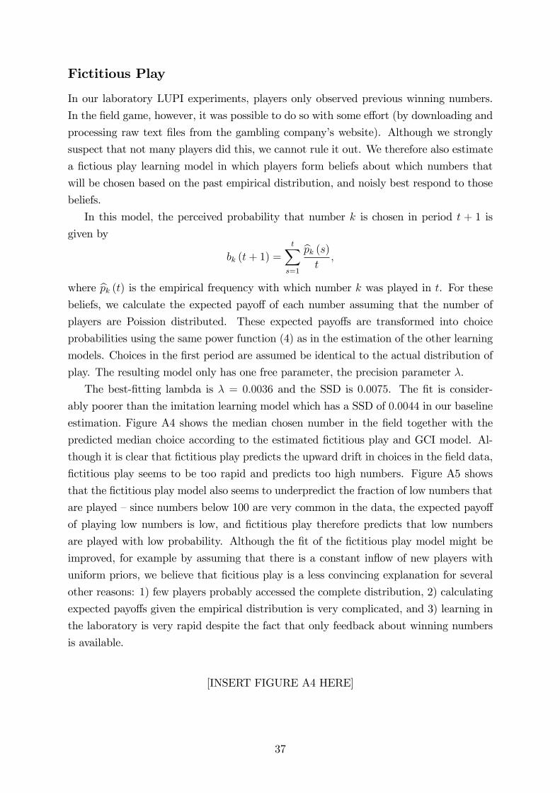
Fictitious Play
In our laboratory LUPI experiments, players only observed previous winning numbers.
In the field game, however, it was possible to do so with some effort (by downloading and
processing raw text files from the gambling company’s website). Although we strongly
suspect that not many players did this, we cannot rule it out. We therefore also estimate
a fictious play learning model in which players form beliefs about which numbers that
will be chosen based on the past empirical distribution, and noisly best respond to those
beliefs.
In this model, the perceived probability that number k is chosen in period t + 1 is
given by
bk (t+ 1) =t∑
s=1
pk (s)
t,
where pk (t) is the empirical frequency with which number k was played in t. For these
beliefs, we calculate the expected payoff of each number assuming that the number of
players are Poission distributed. These expected payoffs are transformed into choice
probabilities using the same power function (4) as in the estimation of the other learning
models. Choices in the first period are assumed be identical to the actual distribution of
play. The resulting model only has one free parameter, the precision parameter λ.
The best-fitting lambda is λ = 0.0036 and the SSD is 0.0075. The fit is consider-
ably poorer than the imitation learning model which has a SSD of 0.0044 in our baseline
estimation. Figure A4 shows the median chosen number in the field together with the
predicted median choice according to the estimated fictitious play and GCI model. Al-
though it is clear that fictitious play predicts the upward drift in choices in the field data,
fictitious play seems to be too rapid and predicts too high numbers. Figure A5 shows
that the fictitious play model also seems to underpredict the fraction of low numbers that
are played —since numbers below 100 are very common in the data, the expected payoff
of playing low numbers is low, and fictitious play therefore predicts that low numbers
are played with low probability. Although the fit of the fictitious play model might be
improved, for example by assuming that there is a constant inflow of new players with
uniform priors, we believe that ficitious play is a less convincing explanation for several
other reasons: 1) few players probably accessed the complete distribution, 2) calculating
expected payoffs given the empirical distribution is very complicated, and 3) learning in
the laboratory is very rapid despite the fact that only feedback about winning numbers
is available.
[INSERT FIGURE A4 HERE]
37

[INSERT FIGURE A5 HERE]
38

Appendix B: Proofs of Results in the Main Text
7.1 Proof of Proposition 1
In addition to the notation and definitions introduced in the main text before Proposition
1 we need the following, taken from Benaïm (1999). For δ > 0, and T > 0, a (δ, T )-pseudo-
orbit from a ∈ X to b ∈ X is a finite sequence of partial trajectories Φt (yi) : 0 ≤ t ≤tii=0,...,k−1, with ti ≥ T , such that d (y0, a) < δ, d
(Φtj (yj) , yj+1
)< δ for j = 0, ..., k − 1,
and yk = b. A point a ∈ X is chain recurrent if there is a (δ, T )-pseudo-orbit from a to a
for every δ > 0, and T > 0. Let Λ ⊆ X be a non-empty invariant set. Φ is called chain
recurrent on Λ if every point x ∈ Λ is a chain recurrent point for Φ|Λ, the restriction of Φ
to Λ. A compact invariant set on which Φ is chain recurrent is called an internally chain
recurrent set. Armed with these concepts, we may prove Proposition 1.
We start by deriving our expressions for the law of motion of p (t).
pk (t+ 1)− pk (t) =Ak (t+ 1)∑Kj=1Aj (t+ 1)
− Ak (t)∑Kj=1Aj (t)
=Ak (t) + rk (t)∑K
j=1 (Aj (t) + rj (t))− pk (t)
=Ak (t) + rk (t)− pk (t)
∑Kj=1 (Aj (t) + rj (t))∑K
j=1 (Aj (t) + rj (t))
=rk (t) + pk (t)
∑Kj=1 rj (t)∑K
j=1Aj (t+ 1).
As mentioned in the main text, let (Ω,F , µ) be a probability space and Ft a filtration,such that Ft is a sub sigma-algebra of F that represents the history of the system up
until the beginning of period t. We can write
p (t+ 1)− p (t) = γ (t+ 1) (F (t) + U (t+ 1)) ,
where the step size is
γ (t+ 1) =1∑K
j=1Aj (t+ 1),
the expected motion is
F (t) = E [rk (t) |Ft]− pk (t)K∑j=1
E [rj (t) |Ft] ,
39

and U (t+ 1) is a stochastic process adapted to Ft;
U (t+ 1) = rk (t)− E [rk (t) |Ft]− pk (t)K∑j=1
(rj (t)− E [rj (t) |Ft]) .
We write γ (t+ 1) and U (t+ 1) but F (t) because the former two terms depend on events
that take place after the beginning of period t, whereas the latter term only depends on
the attractions at the beginning of period t.
Note that E [U (t+ 1) |Ft] = 0, and supt E[‖U (t+ 1)‖2 |Ft
]≤ C for some constant
C. Moreover, for any realization limt→∞ γ (t) = 0,∑∞
t=1 γ (t) = ∞, and∑∞
t=1 (γ (t))2
< ∞. Also F is a bounded locally Lipschitz vector field. Propositions 4.1 and 4.2, with
remark 4.3 in Benaïm (1999) imply that with probability 1, the interpolated process p
is an asymptotic pseudotrajectory of the flow Φ induced by F . Since p (t) : t ≥ 0 isprecompact, the desired result follows from Benaïm’s Theorem 5.7 and Proposition 5.3.
Remark 1 If c = 0 then we face the problem that the step size γ (t) = 1/∑K
i=1 ri (t) is
not guaranteed to satisfy limt→∞ γ (t) = 0,∑∞
t=1 γ (t) = ∞, and∑∞
t=1 γ (t)2 < ∞. Withc = 0 Proposition 1 would continue to hold if almost surely limt→∞ γ (t) = 0, almost
surely∑∞
t=1 γ (t) = ∞, and E[∑∞
t=1 γ (t)2]< ∞. In LUPI, these conditions hold if the
probability of a tie is bounded away from zero. Unfortunately along trajectories towards
the boundary, specifically towards monomorphic states, this need not be the case.
7.2 Proposition 1 with Heterogenous Initial Attractions
We may relax the assumption that all individuals have the same initial attractions. Then,
we have to distinguish the strategy of individual i, denoted σi, from the average strategy
in the population;
p =1
m
m∑i=1
σi.
We have
σik (t+ 1)− σik (t) =rk (t) + σik (t)
∑Kj=1 rj (t)∑K
j=1
(Aij (t) + rj (t)
)=
rk (t) + σik (t)∑K
j=1 rj (t)∑Kj=1A
ij (1) +
∑Kj=1
(∑tτ=1 rj (τ)
)=rk (t) + σik (t)
∑Kj=1 rj (t)∑K
j=1
(∑tτ=1 rj (τ)
) +O
1(∑Kj=1
(∑tτ=1 rj (τ)
))2 .
40

Next, use this to find
pk (t+ 1)− pk (t)
=1
m
m∑i=1
rk (t) + σik (t)∑K
j=1 rj (t)∑Kj=1
(Aij (t) + rj (t)
)=rk (t) +
(1m
∑mi=1 σ
ik (t)
)∑Kj=1 rj (t)∑K
j=1
(∑tτ=1 rj (τ)
) +O
1(∑Kj=1
(∑tτ=1 rj (τ)
))2
=1∑K
j=1
(∑tτ=1 rj (τ)
) (rk (t) + pk (t)K∑j=1
rj (t) +O
(1∑K
j=1
(∑tτ=1 rj (τ)
))) .We can write
p (t+ 1)− p (t) = γ (t+ 1) (F (t) + U (t+ 1) + b (t+ 1)) ,
where F (t) and U (t+ 1) are defined as before, the step size is slightly modified (initial
attractions are removed),
γ (t+ 1) =1∑K
j=1
(∑tτ=1 rj (τ)
) ,and the new term is
b (t+ 1) = O
(1∑K
j=1
(∑tτ=1 rj (τ)
)) .(We write γ (t+ 1), U (t+ 1), and b (t+ 1), but F (t), because the former three terms
depend on events that take place after the beginning of period t whereas the latter term
only depends on the attractions at the beginning of period t.) Note that limt→∞ b (t) = 0.
With the added help of remark 4.5 in Benaïm (1999), the proof of Proposition 1 can be
used again.
7.3 Proof of Proposition 3
We start by noting that the dynamic (7) can be rewritten as follows
pk = npk
(πck (p)−
K∑j=1
pj(πcj (p)
)), (10)
where
πci (p) = πi (p) +c
npi.
41

We may consider an auxiliary perturbed LUPI game with expected payoffs πci (p) rather
than πi (p) for all i. Hence, the perturbed replicator dynamic for a Poisson LUPI game
can be interpreted as the unperturbed replicator dynamic for the perturbed Poisson LUPI
game. It is immediate that (7) has a rest point pc∗ at which πi (p) + cnpi
= πi (pc∗) for all
i. As c→ 0, this rest point converges to the Nash equilibrium of the unperturbed game.
7.3.1 Part 1
We show that the perturbed replicator dynamic (7) has a unique interior rest point pc∗,
by showing that the auxiliary perturbed Poisson LUPI game has a unique symmetric
interior equilibrium pc∗.
Existence follows from Myerson (1998). Full support is ensured by the noise term. To
see this, note that
limpk→0
∂πk (p)
∂pk= lim
pk→0
−n ∏i∈1,...,k−1
(1− npie−npi
)e−npk − c
np2k
= −∞.
In equilibrium, the expected payoff is the same for each action, so
πk+1(p) = e−npk+1k∏i=1
(1− npie−npi
)+
c
npk+1
= e−npkk−1∏i=1
(1− npie−npi
)+
c
npk= πk(p),
or equivalently,
enpk+1
enpk= enpk+1
cn
(1
pk+1− 1
pk
)k−1∏i=1
(1− npie−npi)+(1− npke−npk
).
Taking logarithms on both sides
pk+1 − pk =1
nln
enpk+1cn
(1
pk+1− 1
pk
)k−1∏i=1
(1− npie−npi)+(1− npke−npk
) . (11)
Note that as c→ 0, the left-hand side approaches 1n
ln (1− npke−npk). Since (1− npke−npk) ∈(0, 1) for all p ∈ int (∆), there is some c (k) such that if c < c (k), then we have1n
ln (1− npke−npk) < 0 for the equilibrium p. This implies that pk+1 < pk. We can
42
establish such a bound c (k) for each k. Let c = mink c (k), so that if c < c then pk+1 < pk
for all k. For every candidate equilibrium value of p1 the relationship (11) recursively
determines all equilibrium probabilities. Since the probabilities sum to one and since
pk+1 < pk for all k, there is a unique equilibrium.
7.3.2 Part 2
Propositions 1 and 2 together imply that the realization of the stochastic GCI process
almost surely converges to a compact invariant set that admits no proper attractor under
the flow induced by the perturbed replicator dynamic (7). Part 1 implies that the only
candidate rest point in the interior is the perturbed Nash equilibrium.
7.3.3 Part 3
To rule out convergence to the boundary, recall that the initial attractions are strictly
positive. Since no boundary point is a Nash equilibrium, the proofs of Lemma 3 and
Proposition 3 in Hopkins and Posch (2005) can be adapted; for instance one may consider
the unperturbed dynamic in the perturbed game (defined by the perturbed payoffs πc).
If p′ 6= pc∗, then p′ is not a Nash equilibrium of the perturbed game. If a point p′ is not
a Nash equilibrium, then the Jacobian for the replicator dynamic, evaluated at p′, has at
least one strictly positive eigenvalue. Hopkins and Posch (2005) show that this rules out
convergence. For a related point, see Beggs (2005).
7.4 Proof of Proposition 4
Suppose that p is the symmetric Nash equilibrium. Since p has full support πk = π∗ for
all k we have
wk = npkπ∗. (12)
Summing both sides of (12) over k gives∑wk = nπ∗
∑pk = nπ∗.
Dividing the left-hand side of (12) with∑wk and the right-hand side with nπ∗ gives
pk = wk/∑wk.
To prove the other direction, suppose that p is a mixed strategy with full support that
satisfies pk = wk/∑
j wj. Since wk = npkπk we have
pk =npkπk∑
j wj,
or equivalently πk =∑
j wj/n. Since the right-hand side is the same for all k, it must be
43

a mixed strategy equilibrium.
44

Appendix C: A Family of Global Cumulative Imita-
tion (GCI) Models
In order to be able to generalize the learning rule that we defined for LUPI, we define four
different versions of GCI that happen to coincide in LUPI, but which may yield different
predictions in other games. Therefore, we make two further distinctions. First, imitation
may or may not be responsive to the number of people who play different strategies. This
leads us to distinguish frequency-dependent (FD) and frequency-independent (FI) versions
of GCI. The interaction between payoffs and frequencies may take many forms, but, for
simplicity, we assume a multiplicative interaction, i.e. reinforcement in the frequency-
dependent model depends on the total payoffof all players that picked an action. Second,
imitation may be exclusively focused on emulating the winning action, i.e. the action that
obtained the highest payoff, or be responsive to payoff-differences in a proportional way.
Thus, we differentiate between winner—takes-all imitation (W) and payoff-proportional
imitation (P). In total we introduce the following four members of the GCI family: PFI,
PFD, WFD, and WFI.
Under payoff-proportional frequency-independent global cumulative imitation (PFI-
GCI), reinforcements are
rPFIk (t) =
usi (t) + c if si (t) = k for some i,
c otherwise.(13)
Such reinforcements can be calculated based only on information about the payoff that
was received by actions that someone played. Alternatively, players may also have infor-
mation about the number of players playing each strategy. Let mk (t) be the number of
players picking k at time t. This information is utilized by reinforcement under payoff-
proportional frequency-dependent global cumulative imitation (PFD-GCI),
rPFDk (t) =
mk (t) (usi (t) + c) if si (t) = k for some i,
mk (t) c otherwise.(14)
In the LUPI experiments, subjects do not have any information about mk (t) unless
k is the winning number. However, if c = 0 then mk (t) c = 0 so that rPFDk (t) = 0 for
all k other than the winning number. Thus, for c = 0 subjects in our LUPI experiments
could update attractions with reinforcements of the form rPFDk (t).
Next consider imitation that only reinforces the winning actions —the highest earning
action. In line with Roth (1995), we define winner-takes-all frequency-independent global
45

cumulative imitation (WFD-GCI),
rWFIk (t) =
usi (t) + c if si = k ∈ maxsi usi (s (t)) ,
0 otherwise.(15)
Roth does not explicitly add a constant c but he assumes, equivalently, that all payoffs
are strictly positive.
We also define a frequency-dependent version of winner-takes-all imitation (which is
not mentioned in Roth, 1995); winner-takes-all frequency-dependent global cumulative
imitation (WFI-GCI),
rWFDk (t) =
mk (t) (uk (t) + c) if si = k ∈ maxsi usi (s (t)) ,
0 otherwise.(16)
As in the case of rPFD, if c = 0, thenmk (t) c = 0 so that rWFDk (t) = 0 for all k other than
the winning number. Thus, for c = 0, subjects in our LUPI experiments could update
attractions with reinforcements of the form rWFDk (t).
Recall that k∗ (s) denotes the winning number under strategy profile s. In LUPI, all
reinforcement factors become the same in the limit as c→ 0.
Proposition 5 In LUPI
limc→0
rPFIk (t) = limc→0
rPFDk (t) limc→0
= rWFIk (t) lim
c→0= rWFD
k (t) =
1 if k = k∗ (s (t))
0 otherwise..
Proof. Follows from the fact that in LUPI, mk (t) = 1 for winning k and uk (t) = 0
for losing k. Q.E.D.
Proposition 5 means that we are unable to distinguish the members of the GCI family
in the LUPI game. However, in general, the different members of the GCI-family can be
distinguished as they induce different dynamics. We can show that PFD induces a noisy
replicator dynamic in all games.
Proposition 6 Consider a symmetric game and assume that c > mins∈S u (si, s−i). In
a fixed N-player game, the GCI continuous time dynamic with PFD-reinforcement (14)
is
pk = Npk
(πk (p)−
K∑j=1
pjπj (p)
)+ c (1−Kpk) .
In a Poisson n-player game, the GCI continuous time dynamic with PFD-reinforcement
(14) is
pk = npk
(πk (p)−
K∑j=1
pjπj (p)
)+ c (1−Kpk) .
46

Proof. Let Xt (k) be the total number of players who are drawn to participate and
choose strategy k in period t. For a given focal individual who is drawn to play the
game, let Yt (k) be the number of other players who pick k in period t. In the Poisson
game, the ex ante probability of Xt(k) = m is equal to the probability that Yt(k) = m
conditional on the focal individual being drawn to play. This is due to the environmental
equivalence-property of Poisson games (Myerson, 1998). However in a game with a fixed
number of N players, this is not the case.
We now derive the expected reinforcement ρPFD. To simplify the exposition, we
suppress the reference to Ft. For both fixed and Poisson distributed number of players,we have
E[rPFDk (t) |Ft
]=
N∑j=1
Pr (X (k) = j)E[rPFDk (s) |X (k) = j
]+ Pr (X (k) = 0) (c · 0)
=N∑j=1
Pr (X (k) = j)E [j · (uk (t) + c) |Y (k) = j − 1 ∧X (k) = j]
=N−1∑j=0
Pr (X (k) = j + 1)E [(j + 1) (uk (t) + c) |Y (k) = j ∧X (k) = j + 1] . (17)
For fixed N-player games, we need to translate from Pr (X (k) = j + 1) to Pr (Y (k) = j).
Use
Pr (Y (k) = j) =
(N − 1
j
)pjk (1− pk)N−1−j
=(n− 1)!
j! (n− 1− j)!pjk (1− pk)N−1−j ,
to obtain
Pr (X (k) = j + 1) =
(N
j + 1
)pj+1k (1− pk)N−(j+1)
=N !
(j + 1)! (N − (j + 1))!pj+1k (1− pk)N−j−1
=Npkj + 1
(N − 1)!
j! (N − j − 1)!pjk (1− pk)N−j−1
=Npkj + 1
Pr (Yi (k) = j) .
47

Plugging this into (17) yields
E[rPFDk (t) |Ft
]=
N−1∑j=0
Npkj + 1
Pr (Yi (k) = j)E [(j + 1) (uk (t) + c) |Y (k) = j ∧X (k) = j + 1]
= Npk
N−1∑j=0
Pr (Yi (k) = j)E [(uk (t) + c) |Y (k) = j ∧X (k) = j + 1] ,
or
E[rPFDk (t) |Ft
]= Npk (πk (p (t)) + c) . (18)
Plugging (18) into the general stochastic approximation result (6) gives the desired result
for fixed N -player games.
For Poisson-distributed N , we have
Pr (X (k) = j + 1) =enpk (npk)
j+1
(j + 1)!=
npkj + 1
enpk (npk)j
j!=
npkj + 1
Pr (X (k) = j + 1) .
Plugging this into (17) yields
E[rPFDk (t) |Ft
]=
N−1∑j=0
npkj + 1
Pr (X (k) = j + 1)E [(j + 1) (uk (t) + c) |Y (k) = j ∧X (k) = j + 1]
= npk
N−1∑j=0
Pr (X (k) = j + 1)E [(uk (t) + c) |Y (k) = j ∧X (k) = j + 1]
= npk (πk (p (t)) + c) .
Using this in the general stochastic approximation result (6) gives the desired result for
Poisson games. Q.E.D.
The other three GCI models —PFI, WFI and WFD —do not generally lead to any
version of the replicator dynamic. This can be verified by calculating the expected re-
inforcement and plugging it into equation (6). The different models also differ in their
informational requirements: WDI requires the least feedback, whereas PFD requires the
most. Nevertheless, players could still use all four models in the LUPI game although
they only receive feedback about the action that obtained the highest payoff, i.e. the
winner. Since players can infer the payoff of all other players (zero unless they win), they
can use both winner-imitation and proportional imitation. Moreover, even though they
only know the number of individuals who picked the winning action (one individual),
they are still able to compute the product of payoff and the number of players for all
48

actions (since it is zero for all non-winning actions). For this reason, they are able to use
both frequency dependent and frequency independent imitation.
49

Appendix D: Global Convergence Local Stability
7.5 Global Convergence
In the main text it is established that if the stochastic GCI-process converges to a point
then it must converge to (a perturbed version of) the unique interior equilibrium. In order
to establish that the process does indeed converge to this point and not to something else
than a point —e.g. a periodic orbit —we simulated the learning process. As explained in
Section 3.3 we used the lab parameters K = 99 and n = 26.9, and randomly drew 100
different initial conditions. For each initial condition, we ran the process for 10 million
rounds. Figure D1 shows the resulting distribution at the end of these 10 million rounds,
averaged over the 100 initial conditions.
[INSERT FIGURE D1 HERE]
7.6 Local Stability
Having demonstrated global convergence numerically, the remainder of this Appendix
explores the local stability properties of the unique Nash equilibrium, using a combination
of analytical and numerical methods.
7.6.1 Analytical Methods
Local stability can be determined by studying the Jacobian Dπ (p). An interior equi-
librium p∗ is asymptotically stable under the replicator dynamic, and an evolutionarily
stable strategy, if its associated Jacobian, Dπ (p∗), is negative definite with respect to the
tangent space. With K strategies, the tangent space is RK0 = v ∈ RK :∑
i vi = 0 soan interior equilibrium is asymptotically stable if v′Dπ (p∗) v < 0 for all v ∈ RK0 , v 6= 0.
See e.g. Sandholm (2011), theorem 8.4.1.
We will first prove stability in the unperturbed case and then use a continuity argu-
ment to prove stability under the perturbed replicator dynamic.
Lemma 1 Let
Z =
−2z1 − 4 −z2 − 2 −z3 − 2 · · · −zK−1 − 2
−z2 − 2 −2z2 − 4 −z3 − 2 · · · −zK−1 − 2
−z3 − 2 −z3 − 2 −2z3 − 4 · · · −zK−1 − 2...
......
. . ....
−zK−1 − 2 −zK−1 − 2 −zK−1 − 2 · · · −2zK−1 − 4
, (19)
50

where, for all i,
zi =npi − 1
enpi − npi.
The Jacobian Dπ (p∗) is negative definite w.r.t. the tangent space if and only if all
eigenvalues matrix Z are negative.
Proof. In the Poisson case, we have
∂πk (p)
∂pj=
n(npj−1)e−npj1−npje−npj
∏i∈1,...,k−1
(1− npie−npi) e−npk if j < k
−n∏
i∈1,...,k−1
(1− npie−npi) e−npk if j = k
0 if j > k
,
so the n× n Jacobian can be written
Dπ (p) = n
−π1 0 0 · · · · · · 0
z1π2 −π2 0 · · · · · · 0
z1π3 z2π3 −π3 · · · · · · 0...
......
. . ....
......
.... . .
...
z1πK z2πK z3πK · · · · · · −πK
,
where
zi =npi − 1
enpi − npi.
Let P be the n× (n− 1)-matrix defined by
pij =
1 if i = j and i, j < n
0 if i 6= j and i, j < n
−1 if i = n
.
Checking that Dπ (p) is negative definite w.r.t. the tangent space RK0 (or a subset of
the tangent space) is the same as checking whether the transformed matrix P′Dπ (p)P
is negative definite w.r.t. the space RK−1; see Weissing (1991). At the equilibrium p∗, we
have πi (p∗) = πNE for all i. Using the transformation matrix P yields
P′Dπ (p∗)P = nπNE
−z1 − 2 −z2 − 1 −z3 − 1 · · · −zK−1 − 1
−1 −z2 − 2 −z3 − 1 · · · −zK−1 − 1
−1 −1 −z3 − 2 · · · −zK−1 − 1...
......
. . ....
−1 −1 −1 · · · −zK−1 − 2
.
51

The matrix P′Dπ (p∗)P is negative definite if and only if the following symmetric matrix
is negative definite.
Z =1
nπNE(P′Dπ (p∗)P+ (P′Dπ (p∗)P)
′) .This yields the matrix (19). Q.E.D.
To connect stability under the (unperturbed) replicator dynamic with stability under
the perturbed dynamic, we need the following lemma.
Lemma 2 Suppose that p∗ is locally asymptotically stable under the (unperturbed) repli-cator dynamic. There is some c such that if c < c, then the perturbed equilibrium pc∗ is
locally asymptotically stable under the perturbed replicator dynamic.
Proof. Consider
Zc =1
nπc (pc∗)
(P′Dπ (pc∗)P+ (P′Dπ (pc∗)P)
′) .Since pc∗ is continuous in c both πc (pc∗) andDπ (pc∗) are continuous in c. Thus, the entries
of Zc are continuous in c, and since the eigenvalues are the roots of the characteristic
polynomial det (Zc − λI) = 0, they are continous in the entries of Zc. Since (by Lemma
1) the eigenvalues of Z = Z0 are strictly negative, there is some c > 0 such that if c < c
then the eigenvalues of Zc are strictly negative. Q.E.D.
Lemmas 1 and 2 imply that if all eigenvalues of Z are negative, then there is some
c such that if c < c then the perturbed equilibrium pc∗ is locally asymptotically stable
under the perturbed replicator dynamic. If pc∗ is indeed locally asymptotically stable
under the perturbed replicator dynamic, then theorem 7.3 of Benaïm (1999) establishes
that GCI converges to the perturbed Nash equilibrium with positive probability. We may
conclude that:
Proposition 7 If all eigenvalues of Z are negative, then p∗ is an evolutionarily stable
strategy, and there is some c such that if c < c then with positive probability, the sto-
chastic GCI-process converges to the unique interior rest point of the perturbed replicator
dynamic.
7.6.2 Numerical Methods
In order to evaluate the definiteness of Z, we have to resort to numerical methods. First,
we compute the vector p using the Brent-Dekker root-finding method for greatest pre-
cision. Next, the matrix Z is created from the vector p, and negated. By negating the
matrix (and thus its eigenvalues), we can instead check whether the matrix is positive
52

definite instead of negative definite. For this purpose, we can use a Cholesky decomposi-
tion, which is faster than actually computing eigenvalues. We used the generic LAPACK
and BLAS system in FORTRAN, and cross-checked using the optimized Atlas and Open-
BLAS implementations in C with the same results.
For K = 100, the eigenvalues can be computed with suffi cient precision to warrant
the conclusion that all eigenvalues are indeed negative. For K = 99, 999, as in the field
game, the calculations are less reliable. For K = 99, 999 it seems that we need numerical
precision beyond 64 bits (double-precision floating points) in order correctly compute the
result. This will require a tremendous amount of memory. By way of explanation, assume
all operations are on double-precision floating point numbers. Thus, given a matrix of
size K = 99, 999, this comes to 99, 998 × 99, 998 = 9, 999, 600, 004 numbers, or ˜9 GB
worth of numbers, each of which is 8 B (64 bits). With bookkeeping in place, that’s 74
GB of memory.
Thus, we conclude that the Nash equilibrium is locally asymptotically stable, at least
for the lab parameters. It follows that if the level of noise is small enough then with posi-
tive probability the stochastic GCI-process converges to the perturbed Nash equilibrium.
Conclusion 1 For K = 100, p∗ is an evolutionarily stable strategy, and there is some c
such that if c < c then, with positive probability, the stochastic GCI-process converges to
the unique interior rest point of the perturbed replicator dynamic.
53

Appendix E: Additional Empirical Results
[INSERT FIGURES E1-E8 HERE.]
54
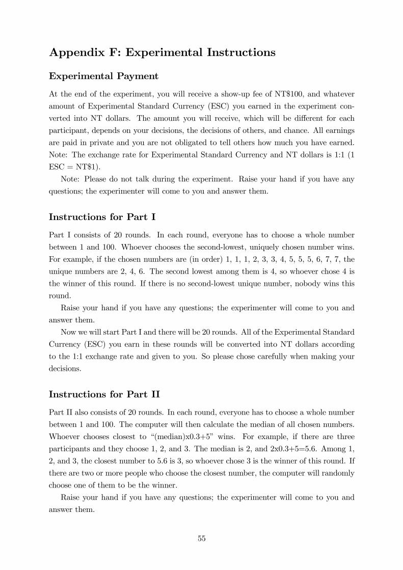
Appendix F: Experimental Instructions
Experimental Payment
At the end of the experiment, you will receive a show-up fee of NT$100, and whatever
amount of Experimental Standard Currency (ESC) you earned in the experiment con-
verted into NT dollars. The amount you will receive, which will be different for each
participant, depends on your decisions, the decisions of others, and chance. All earnings
are paid in private and you are not obligated to tell others how much you have earned.
Note: The exchange rate for Experimental Standard Currency and NT dollars is 1:1 (1
ESC = NT$1).
Note: Please do not talk during the experiment. Raise your hand if you have any
questions; the experimenter will come to you and answer them.
Instructions for Part I
Part I consists of 20 rounds. In each round, everyone has to choose a whole number
between 1 and 100. Whoever chooses the second-lowest, uniquely chosen number wins.
For example, if the chosen numbers are (in order) 1, 1, 1, 2, 3, 3, 4, 5, 5, 5, 6, 7, 7, the
unique numbers are 2, 4, 6. The second lowest among them is 4, so whoever chose 4 is
the winner of this round. If there is no second-lowest unique number, nobody wins this
round.
Raise your hand if you have any questions; the experimenter will come to you and
answer them.
Now we will start Part I and there will be 20 rounds. All of the Experimental Standard
Currency (ESC) you earn in these rounds will be converted into NT dollars according
to the 1:1 exchange rate and given to you. So please chose carefully when making your
decisions.
Instructions for Part II
Part II also consists of 20 rounds. In each round, everyone has to choose a whole number
between 1 and 100. The computer will then calculate the median of all chosen numbers.
Whoever chooses closest to “(median)x0.3+5” wins. For example, if there are three
participants and they choose 1, 2, and 3. The median is 2, and 2x0.3+5=5.6. Among 1,
2, and 3, the closest number to 5.6 is 3, so whoever chose 3 is the winner of this round. If
there are two or more people who choose the closest number, the computer will randomly
choose one of them to be the winner.
Raise your hand if you have any questions; the experimenter will come to you and
answer them.
55

Now we will start Part II and there will be 20 rounds. All of the Experimental
Standard Currency (ESC) you earn in these rounds will be converted into NT dollars
according to the 1:1 exchange rate and given to you. So please chose carefully when
making your decisions.
Instructions for Part III
Part III consists of 20 rounds. In each round, everyone has to choose a whole number
between 1 and 100. Whoever chooses closest to 50, uniquely chosen number wins. If
there are two numbers of the same distance to 50, the larger number wins. For example,
you win if there are two or more who choose 50 and you uniquely choose 51. If there are
two or more who choose 50 and 51, we will have to check (in order) if anyone uniquely
chose 49, 52, 48, etc.
[INSERT FIGURE F1 HERE]
If no number is uniquely chosen, nobody wins in this round.
Raise your hand if you have any questions; the experimenter will come to you and
answer them.
Now we will start Part III and there will be 20 rounds. All of the Experimental
Standard Currency (ESC) you earn in these rounds will be converted into NT dollars
according to the 1:1 exchange rate and given to you. So please chose carefully when
making your decisions.
56

Figure 1. Bartlett similarity window (k* = 10, W = 3).
Figure 2. Movement towards equilibrium in the field LUPI game. Daily values of the proportion of empirical density that lies below the predicted equilibrium density. In equilibrium the expected value of the measure is about 0.87.

Figure 3. The relationship between previous winning numbers and chosen numbers in the field LUPI game. The difference between the winning numbers at time t and time t – 1 compared to the difference between the average chosen number at time t + 1 and time t.
Figure 4. Estimated reinforcement factors in the field LUPI game. The winning number is excluded. Black solid line represents a moving average over 201 numbers.

Figure 5a. Daily empirical densities (bars), estimated learning model (solid lines), Poisson-Nash equilibrium (dashed line), and the winning number in the previous period (dotted lines) for the field LUPI game day 2-25. Estimated values W = 1999, and λ = 1. To improve readability the empirical densities have been smoothed with a moving average over 201 numbers.

Figure 5b. Daily empirical densities (bars), estimated learning model (solid lines), Poisson-Nash equilibrium (dashed line), and winning number in the previous period (dotted lines) for the field LUPI game day 26-49. Estimated values W = 1999, and λ = 1. To improve readability the empirical densities have been smoothed with a moving average over 201 numbers.

Figure 6. Movement towards equilibrium in the laboratory LUPI game. Per-period values of the proportion of empirical distribution that lies below the equilibrium distribution. Fitted linear trends (black dashed lines). In equilibrium the expected value of the measure is about 0.74 (grey dashed horizontal lines).
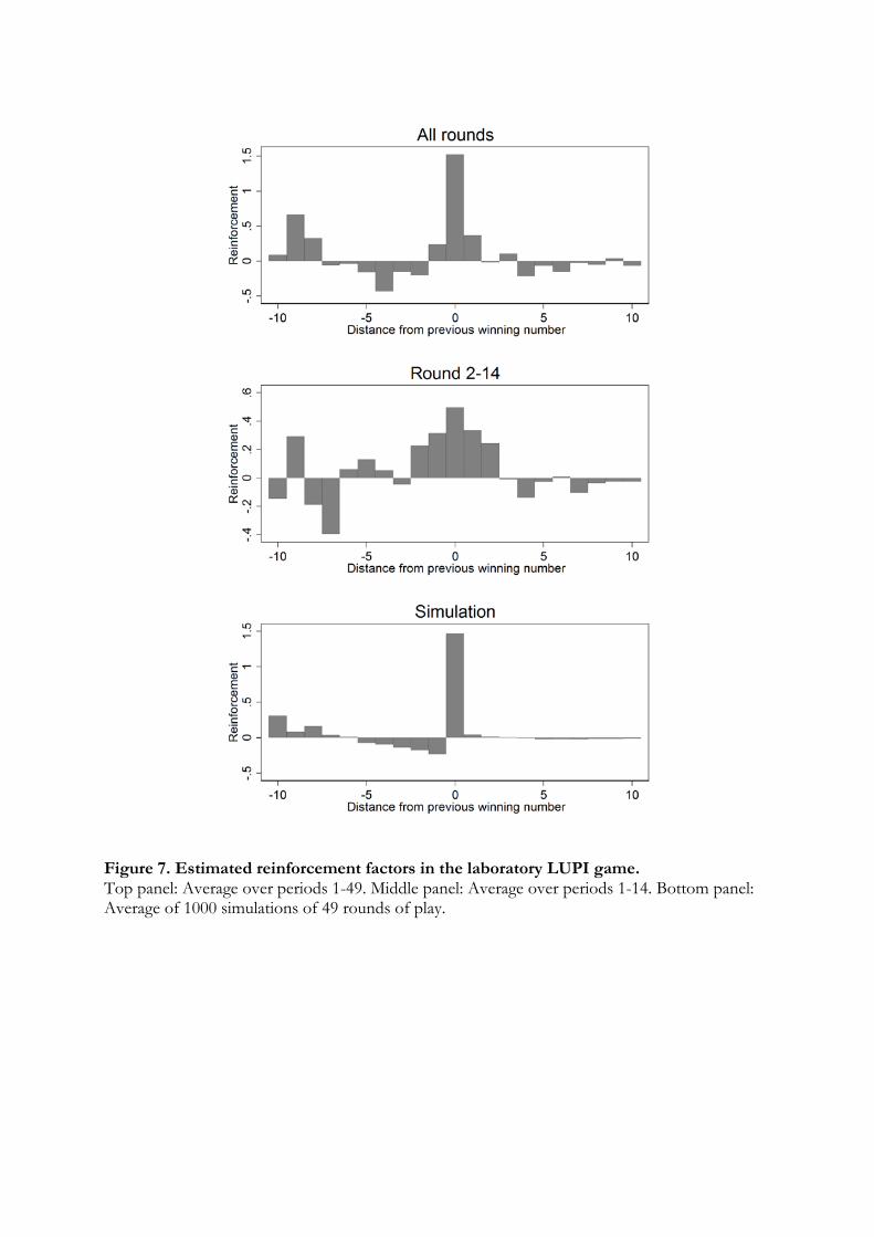
Figure 7. Estimated reinforcement factors in the laboratory LUPI game. Top panel: Average over periods 1-49. Middle panel: Average over periods 1-14. Bottom panel: Average of 1000 simulations of 49 rounds of play.

Figure 8. Empirical densities (bars) and theoretical benchmark (solid lines) for periods 1-3 and 16-20 in the SLUPI, pmBC and CUPI games. The theoretical benchmark is the Poisson-Nash equilibrium for CUPI and the simulated similarity-based GCI model for the SLUPI game (period 20 prediction averaged over 100,000 simulations with W=5 and λ = 1).
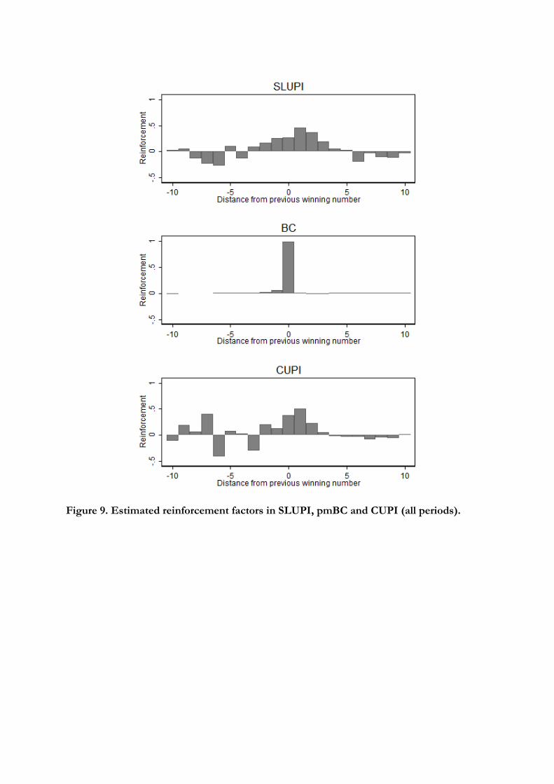
Figure 9. Estimated reinforcement factors in SLUPI, pmBC and CUPI (all periods).
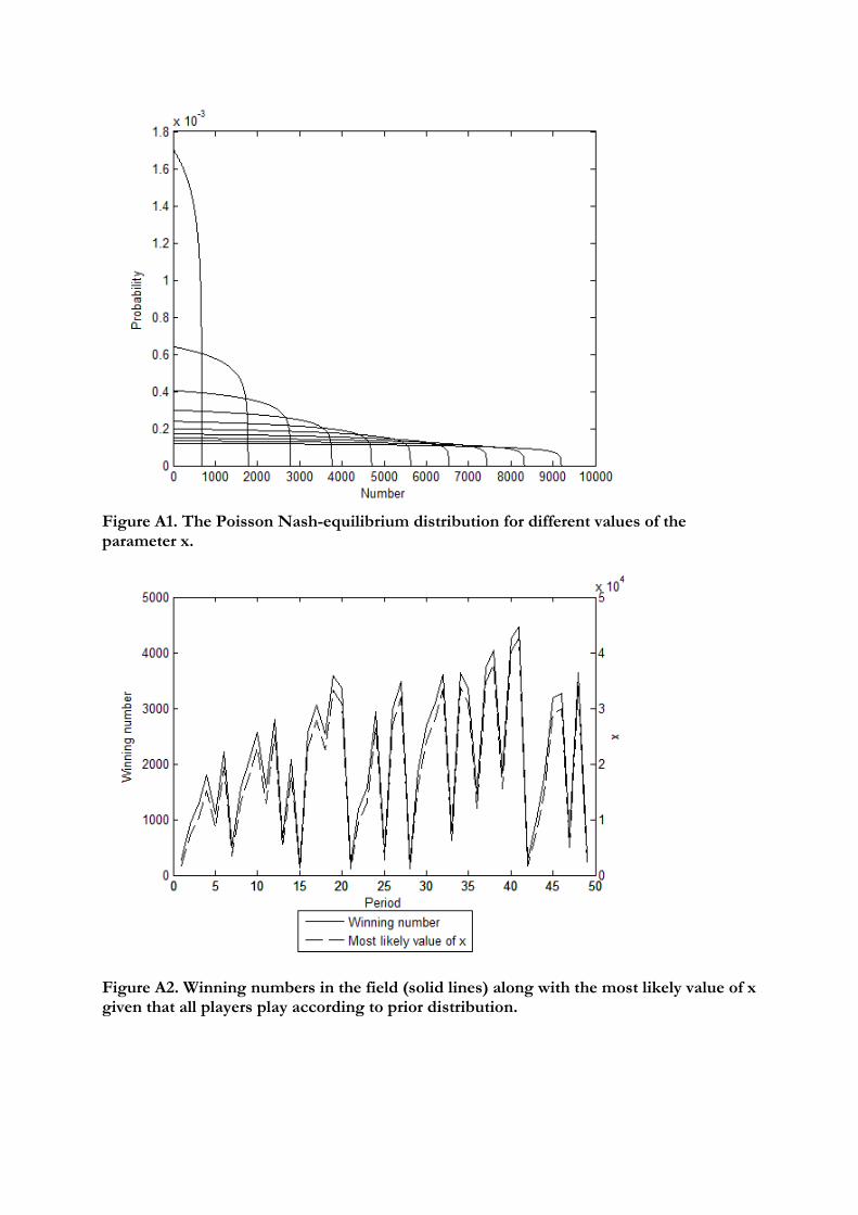
Figure A1. The Poisson Nash-equilibrium distribution for different values of the parameter x.
Figure A2. Winning numbers in the field (solid lines) along with the most likely value of x given that all players play according to prior distribution.

Figure A3. Evolution of posterior beliefs about parameter x.
Figure A4. Actual and predicted number chosen in the field LUPI game (period 2-49) The solid line shows the actual median played, the dashed line the predicted median from the baseline GCI baseline estimation, and the dotted line the predicted median according to the estimated fictitious play learning model.

Figure A5. Actual and predicted numbers below 100 in the field LUPI game (period 2-49) The solid line shows the actual fraction of numbers below 100, the dashed line the predicted fraction of numbers below 100 from the baseline GCI baseline estimation, and the dotted line the corresponding prediction of the estimated fictitious play learning model.
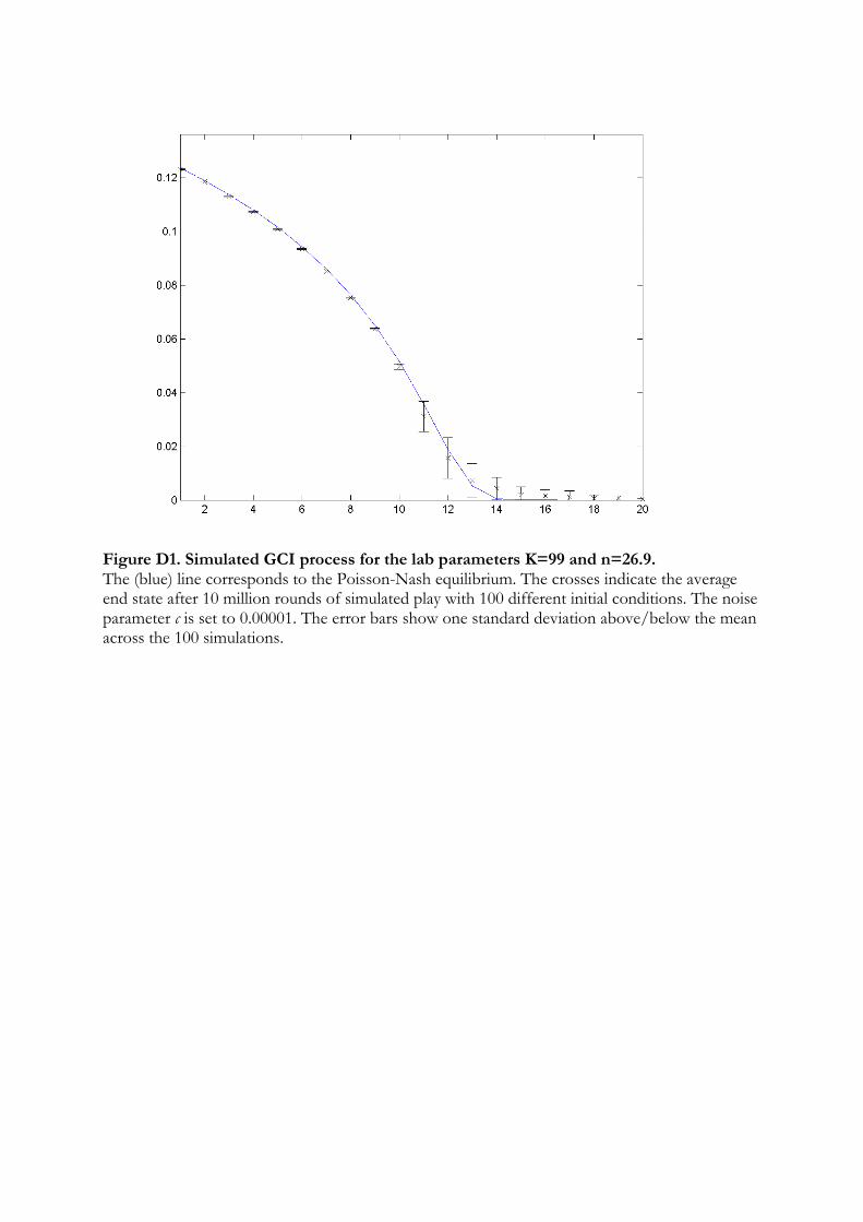
Figure D1. Simulated GCI process for the lab parameters K=99 and n=26.9. The (blue) line corresponds to the Poisson-Nash equilibrium. The crosses indicate the average end state after 10 million rounds of simulated play with 100 different initial conditions. The noise parameter c is set to 0.00001. The error bars show one standard deviation above/below the mean across the 100 simulations.

Figure E1. Distribution of chosen (thick solid line) and winning (thin solid line) numbers in all sessions from period 25 and onwards and the Poisson Nash equilibrium (dashed line).
-15
-10
-50
510
Mea
n nu
mbe
r cha
nge
-50
5W
inni
ng n
umbe
r cha
nge
0 5 10 15t
-4-2
02
4M
ean
num
ber c
hang
e
-10
-50
5W
inni
ng n
umbe
r cha
nge
0 5 10 15t
-3-2
-10
12
Mea
n nu
mbe
r cha
nge
-20
-10
010
20W
inni
ng n
umbe
r cha
nge
0 5 10 15t
-4-2
02
4M
ean
num
ber c
hang
e
-10
-50
510
Win
ning
num
ber c
hang
e
0 5 10 15t
Figure E2. The effect of winning numbers on chosen numbers in LUPI The difference between the winning numbers at time t and time t-1 (solid line) compared to the difference between the average chosen number at time t+1 and time t (dashed line). Data from one periond in the first session excluded to make figure readable (winner was 67).
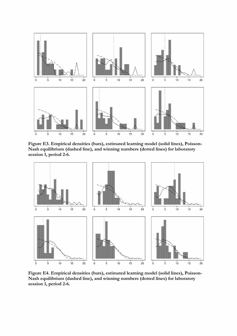
Figure E3. Empirical densities (bars), estimated learning model (solid lines), Poisson-Nash equilibrium (dashed line), and winning numbers (dotted lines) for laboratory session 1, period 2-6.
Figure E4. Empirical densities (bars), estimated learning model (solid lines), Poisson-Nash equilibrium (dashed line), and winning numbers (dotted lines) for laboratory session 1, period 2-6.
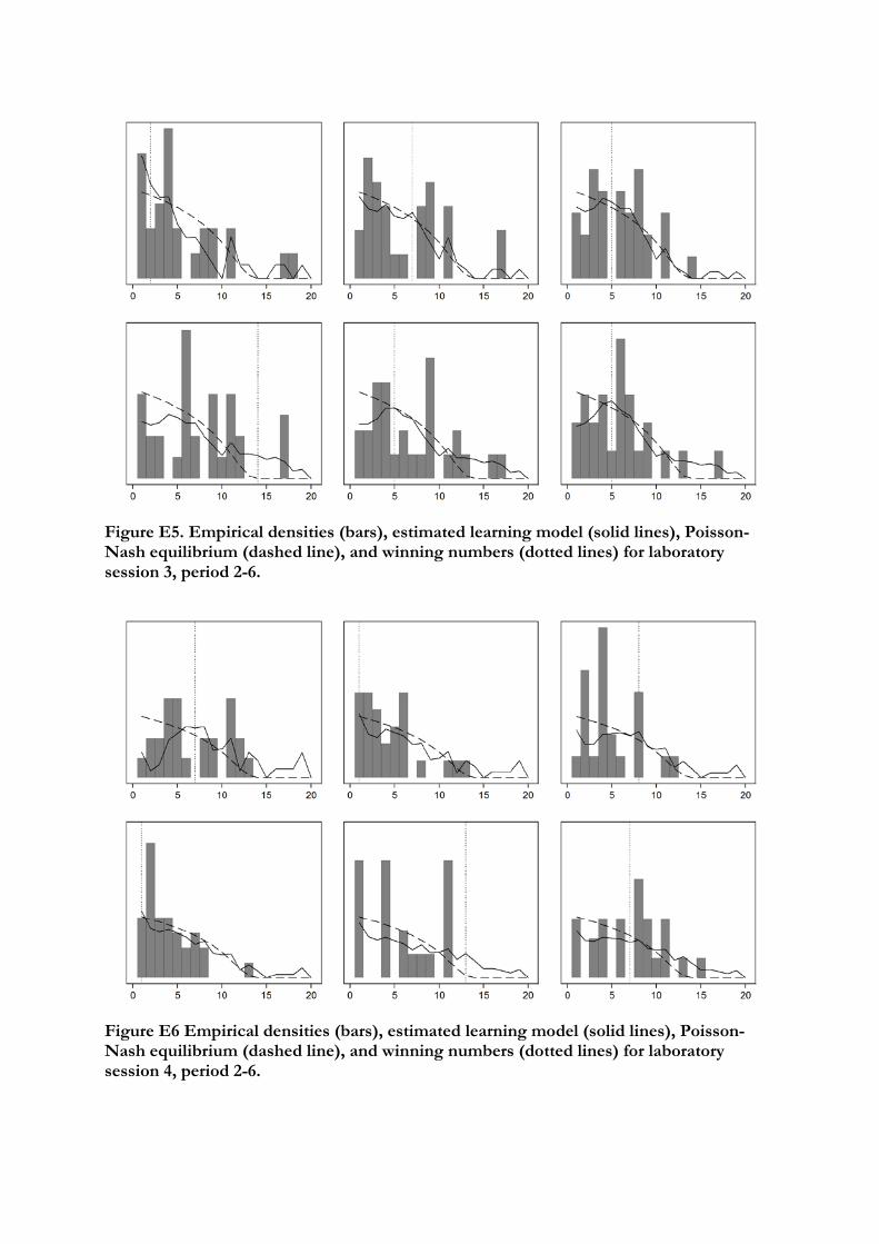
Figure E5. Empirical densities (bars), estimated learning model (solid lines), Poisson-Nash equilibrium (dashed line), and winning numbers (dotted lines) for laboratory session 3, period 2-6.
Figure E6 Empirical densities (bars), estimated learning model (solid lines), Poisson-Nash equilibrium (dashed line), and winning numbers (dotted lines) for laboratory session 4, period 2-6.

Figure E7: The effect of winning numbers on chosen numbers in SLUPI, pmBC and CUPI. The difference between the winning numbers at time t and time t-1 (solid line) compared to the difference between the average chosen number at time t+1 and time t (dashed line). Winning numbers that change more than 10 numbers is shown as 10/-10 in graph. The strategy space in CUPI has been transformed as described in the main text.

Figure E8. Estimated reinforcement factors in SLUPI, pmBC and CUPI including only period 1-5.

Figure F1. Figure included in the CUPI game instructions.