Learning Bayesian Networks with the bnlearn R Package · 2 Learning Bayesian Networks with the...

JSS Journal of Statistical SoftwareMMMMMM YYYY, Volume VV, Issue II. http://www.jstatsoft.org/

Learning Bayesian Networks with the bnlearn RPackage

Marco ScutariUniversity of Padova

Abstract

bnlearn is an R package (R Development Core Team 2009) which includes several algo-rithms for learning the structure of Bayesian networks with either discrete or continuousvariables. Both constraint-based and score-based algorithms are implemented, and canuse the functionality provided by the snow package (Tierney et al. 2008) to improve theirperformance via parallel computing. Several network scores and conditional independencealgorithms are available for both the learning algorithms and independent use. Advancedplotting options are provided by the Rgraphviz package (Gentry et al. 2010).

Keywords: bayesian networks, R, structure learning algorithms, constraint-based algorithms,score-based algorithms, conditional independence tests.

1. Introduction

In recent years Bayesian networks have been used in many fields, from On-line AnalyticalProcessing (OLAP) performance enhancement (Margaritis 2003) to medical service perfor-mance analysis (Acid et al. 2004), gene expression analysis (Friedman et al. 2000), breastcancer prognosis and epidemiology (Holmes and Jain 2008).

The high dimensionality of the data sets common in these domains have led to the develop-ment of several learning algorithms focused on reducing computational complexity while stilllearning the correct network. Some examples are the Grow-Shrink algorithm in Margaritis(2003), the Incremental Association algorithm and its derivatives in Tsamardinos et al. (2003)and in Yaramakala and Margaritis (2005), the Sparse Candidate algorithm in Friedman et al.(1999), the Optimal Reinsertion in Moore and Wong (2003) and the Greedy Equivalent Searchin Chickering (2002).

The aim of the bnlearn package is to provide a free implementation of some of these structurelearning algorithms along with the conditional independence tests and network scores used

arX

iv:0

908.

3817

v2 [

stat

.ML

] 1

0 Ju

l 201

0

http://www.jstatsoft.org/

2 Learning Bayesian Networks with the bnlearn R Package

to construct the Bayesian network. Both discrete and continuous data are supported. Fur-thermore, the learning algorithms can be chosen separately from the statistical criterion theyare based on (which is usually not possible in the reference implementation provided by thealgorithms’ authors), so that the best combination for the data at hand can be used.

2. Bayesian networks

Bayesian networks are graphical models where nodes represent random variables (the twoterms are used interchangeably in this article) and arrows represent probabilistic dependenciesbetween them (Korb and Nicholson 2004).

The graphical structure G = (V, A) of a Bayesian network is a directed acyclic graph (DAG),where V is the node (or vertex ) set and A is the arc (or edge) set. The DAG defines afactorization of the joint probability distribution of V = {X1, X2, . . . , Xv}, often called theglobal probability distribution, into a set of local probability distributions, one for each variable.The form of the factorization is given by the Markov property of Bayesian networks (Korb andNicholson 2004, section 2.2.4), which states that every random variable Xi directly dependsonly on its parents ΠXi :

P(X1, . . . , Xv) =v∏

i=1

P(Xi |ΠXi) (for discrete variables) (1)

f(X1, . . . , Xv) =v∏

i=1

f(Xi |ΠXi) (for continuous variables). (2)

The correspondence between conditional independence (of the random variables) and graph-ical separation (of the corresponding nodes of the graph) has been extended to an arbitrarytriplet of disjoint subsets of V by Pearl (1988) with the d-separation (from direction-dependentseparation). Therefore model selection algorithms first try to learn the graphical structure ofthe Bayesian network (hence the name of structure learning algorithms) and then estimatethe parameters of the local distribution functions conditional on the learned structure. Thistwo-step approach has the advantage that it considers one local distribution function at atime, and it does not require to model the global distribution function explicitly. Anotheradvantage is that learning algorithms are able to scale to fit high-dimensional models withoutincurring in the so-called curse of dimensionality.

Although there are many possible choices for both the global and the local distribution func-tions, literature have focused mostly on two cases:

• multinomial data (the discrete case): both the global and the local distributions aremultinomial, and are represented as probability or contingency tables. This is by farthe most common assumption, and the corresponding Bayesian networks are usuallyreferred to as discrete Bayesian networks (or simply as Bayesian networks).

• multivariate normal data (the continuous case): the global distribution is multivariatenormal, and the local distributions are normal random variables linked by linear con-straints. These Bayesian networks are called Gaussian Bayesian networks in Geiger andHeckerman (1994), Neapolitan (2003) and most recent literature on the subject.

Journal of Statistical Software 3

Other distributional assumptions lead to more complex learning algorithms (such as the non-parametric approach proposed by Bach and Jordan (2003)) or present various limitations dueto the difficulty of specifying the distribution functions in closed form (such as the approach tolearn Bayesian network with mixed variables by Boettcher and Dethlefsen (2003), which doesnot allow a node associated with a continuous variable to be the parent of a node associatedwith a discrete variable).

3. Structure learning algorithms

Bayesian network structure learning algorithms can be grouped in two categories:

• constraint-based algorithms: these algorithms learn the network structure by analyzingthe probabilistic relations entailed by the Markov property of Bayesian networks withconditional independence tests and then constructing a graph which satisfies the corre-sponding d-separation statements. The resulting models are often interpreted as causalmodels even when learned from observational data (Pearl 1988).

• score-based algorithms: these algorithms assign a score to each candidate Bayesiannetwork and try to maximize it with some heuristic search algorithm. Greedy searchalgorithms (such as hill-climbing or tabu search) are a common choice, but almost anykind of search procedure can be used.

Constraint-based algorithms are all based on the Inductive Causation (IC) algorithm by Vermaand Pearl (1991), which provides a theoretical framework for learning the structure causalmodels. It can be summarized in three steps:

1. first the skeleton of the network (the undirected graph underlying the network structure)is learned. Since an exhaustive search is computationally unfeasible for all but the mostsimple data sets, all learning algorithms use some kind of optimization such as restrictingthe search to the Markov blanket of each node (which includes the parents, the childrenand all the nodes that share a child with that particular node).

2. set all direction of the arcs that are part of a v-structure (a triplet of nodes incident ona converging connection Xj → Xi ← Xk).

3. set the directions of the other arcs as needed to satisfy the acyclicity constraint.

Score-based algorithms on the other hand are simply applications of various general purposeheuristic search algorithms, such as hill-climbing, tabu search, simulated annealing and variousgenetic algorithms. The score function is usually score-equivalent (Chickering 1995), so thatnetworks that define the same probability distribution are assigned the same score.


4. Package implementation

4.1. Structure learning algorithms

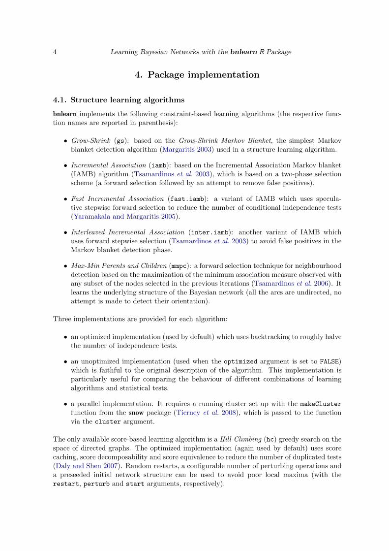
bnlearn implements the following constraint-based learning algorithms (the respective func-tion names are reported in parenthesis):

• Grow-Shrink (gs): based on the Grow-Shrink Markov Blanket, the simplest Markovblanket detection algorithm (Margaritis 2003) used in a structure learning algorithm.

• Incremental Association (iamb): based on the Incremental Association Markov blanket(IAMB) algorithm (Tsamardinos et al. 2003), which is based on a two-phase selectionscheme (a forward selection followed by an attempt to remove false positives).

• Fast Incremental Association (fast.iamb): a variant of IAMB which uses specula-tive stepwise forward selection to reduce the number of conditional independence tests(Yaramakala and Margaritis 2005).

• Interleaved Incremental Association (inter.iamb): another variant of IAMB whichuses forward stepwise selection (Tsamardinos et al. 2003) to avoid false positives in theMarkov blanket detection phase.

• Max-Min Parents and Children (mmpc): a forward selection technique for neighbourhooddetection based on the maximization of the minimum association measure observed withany subset of the nodes selected in the previous iterations (Tsamardinos et al. 2006). Itlearns the underlying structure of the Bayesian network (all the arcs are undirected, noattempt is made to detect their orientation).

Three implementations are provided for each algorithm:

• an optimized implementation (used by default) which uses backtracking to roughly halvethe number of independence tests.

• an unoptimized implementation (used when the optimized argument is set to FALSE)which is faithful to the original description of the algorithm. This implementation isparticularly useful for comparing the behaviour of different combinations of learningalgorithms and statistical tests.

• a parallel implementation. It requires a running cluster set up with the makeCluster

function from the snow package (Tierney et al. 2008), which is passed to the functionvia the cluster argument.

The only available score-based learning algorithm is a Hill-Climbing (hc) greedy search on thespace of directed graphs. The optimized implementation (again used by default) uses scorecaching, score decomposability and score equivalence to reduce the number of duplicated tests(Daly and Shen 2007). Random restarts, a configurable number of perturbing operations anda preseeded initial network structure can be used to avoid poor local maxima (with therestart, perturb and start arguments, respectively).


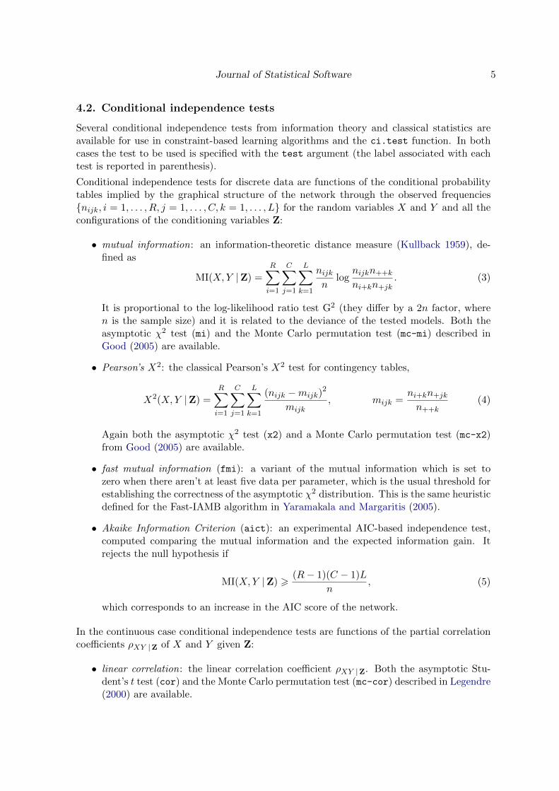
4.2. Conditional independence tests

Several conditional independence tests from information theory and classical statistics areavailable for use in constraint-based learning algorithms and the ci.test function. In bothcases the test to be used is specified with the test argument (the label associated with eachtest is reported in parenthesis).

Conditional independence tests for discrete data are functions of the conditional probabilitytables implied by the graphical structure of the network through the observed frequencies{nijk, i = 1, . . . , R, j = 1, . . . , C, k = 1, . . . , L} for the random variables X and Y and all theconfigurations of the conditioning variables Z:

• mutual information: an information-theoretic distance measure (Kullback 1959), de-fined as

MI(X,Y |Z) =R∑i=1

C∑j=1

L∑k=1

nijkn

lognijkn++k

ni+kn+jk. (3)

It is proportional to the log-likelihood ratio test G2 (they differ by a 2n factor, wheren is the sample size) and it is related to the deviance of the tested models. Both theasymptotic χ2 test (mi) and the Monte Carlo permutation test (mc-mi) described inGood (2005) are available.

• Pearson’s X2: the classical Pearson’s X2 test for contingency tables,

X2(X,Y |Z) =

R∑i=1

C∑j=1

L∑k=1

(nijk −mijk)2

mijk, mijk =

ni+kn+jk

n++k(4)

Again both the asymptotic χ2 test (x2) and a Monte Carlo permutation test (mc-x2)from Good (2005) are available.

• fast mutual information (fmi): a variant of the mutual information which is set tozero when there aren’t at least five data per parameter, which is the usual threshold forestablishing the correctness of the asymptotic χ2 distribution. This is the same heuristicdefined for the Fast-IAMB algorithm in Yaramakala and Margaritis (2005).

• Akaike Information Criterion (aict): an experimental AIC-based independence test,computed comparing the mutual information and the expected information gain. Itrejects the null hypothesis if

MI(X,Y |Z) >(R− 1)(C − 1)L

n, (5)

which corresponds to an increase in the AIC score of the network.

In the continuous case conditional independence tests are functions of the partial correlationcoefficients ρXY |Z of X and Y given Z:

• linear correlation: the linear correlation coefficient ρXY |Z. Both the asymptotic Stu-dent’s t test (cor) and the Monte Carlo permutation test (mc-cor) described in Legendre(2000) are available.


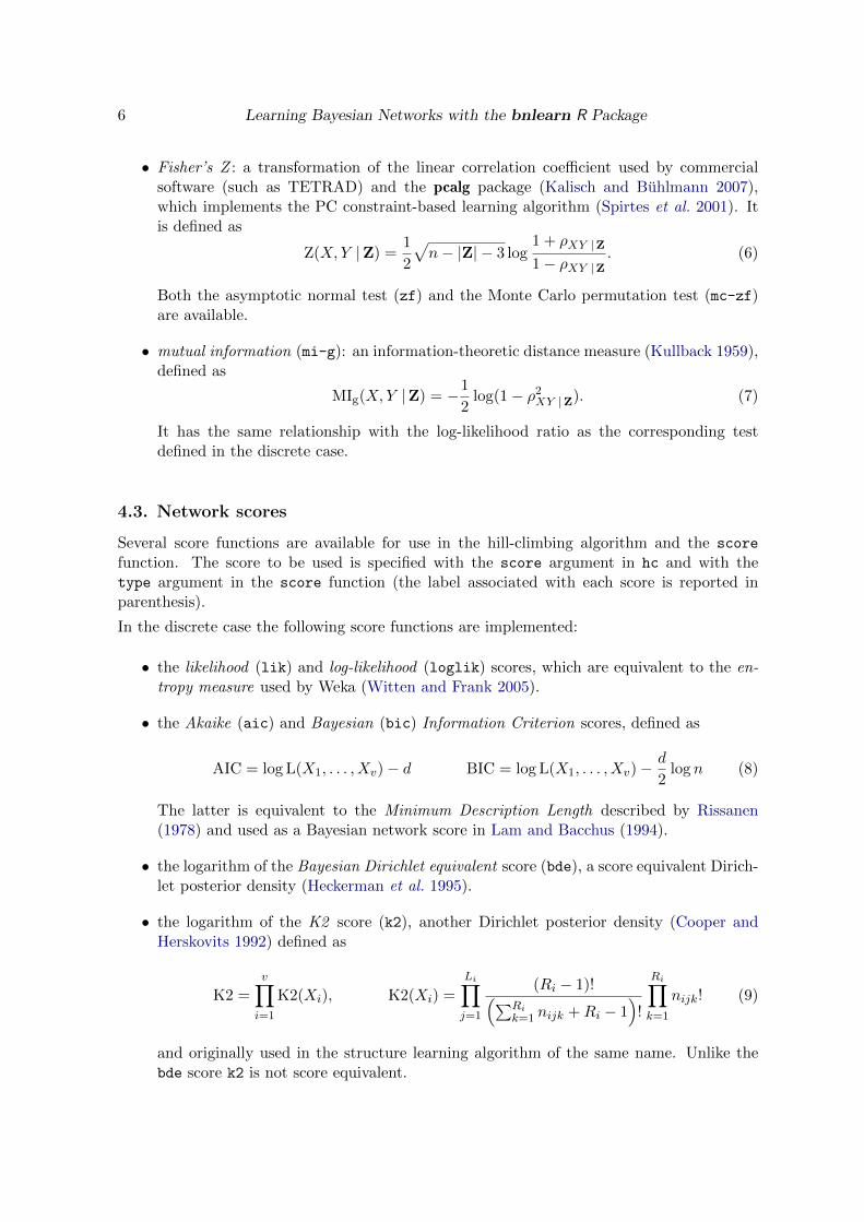
• Fisher’s Z : a transformation of the linear correlation coefficient used by commercialsoftware (such as TETRAD) and the pcalg package (Kalisch and Buhlmann 2007),which implements the PC constraint-based learning algorithm (Spirtes et al. 2001). Itis defined as

Z(X,Y |Z) =1

2

√n− |Z| − 3 log

1 + ρXY |Z

1− ρXY |Z. (6)

Both the asymptotic normal test (zf) and the Monte Carlo permutation test (mc-zf)are available.

• mutual information (mi-g): an information-theoretic distance measure (Kullback 1959),defined as

MIg(X,Y |Z) = −1

2log(1− ρ2XY |Z). (7)

It has the same relationship with the log-likelihood ratio as the corresponding testdefined in the discrete case.

4.3. Network scores

Several score functions are available for use in the hill-climbing algorithm and the score

function. The score to be used is specified with the score argument in hc and with thetype argument in the score function (the label associated with each score is reported inparenthesis).

In the discrete case the following score functions are implemented:

• the likelihood (lik) and log-likelihood (loglik) scores, which are equivalent to the en-tropy measure used by Weka (Witten and Frank 2005).

• the Akaike (aic) and Bayesian (bic) Information Criterion scores, defined as

AIC = log L(X1, . . . , Xv)− d BIC = log L(X1, . . . , Xv)− d

2log n (8)

The latter is equivalent to the Minimum Description Length described by Rissanen(1978) and used as a Bayesian network score in Lam and Bacchus (1994).

• the logarithm of the Bayesian Dirichlet equivalent score (bde), a score equivalent Dirich-let posterior density (Heckerman et al. 1995).

• the logarithm of the K2 score (k2), another Dirichlet posterior density (Cooper andHerskovits 1992) defined as

K2 =

v∏i=1

K2(Xi), K2(Xi) =

Li∏j=1

(Ri − 1)!(∑Rik=1 nijk +Ri − 1

)!

Ri∏k=1

nijk! (9)

and originally used in the structure learning algorithm of the same name. Unlike thebde score k2 is not score equivalent.


The only score available for the continuous case is a score equivalent Gaussian posteriordensity (bge), which follows a Wishart distribution (Geiger and Heckerman 1994).

4.4. Arc whitelisting and blacklisting

Prior information on the data, such as the ones elicited from experts in the relevant fields, canbe integrated in all learning algorithms by means of the blacklist and whitelist arguments.Both of them accept a set of arcs which is guaranteed to be either present (for the former) ormissing (for the latter) from the Bayesian network; any arc whitelisted and blacklisted at thesame time is assumed to be whitelisted, and is thus removed from the blacklist.

This combination represents a very flexible way to describe any arbitrary set of assumptionson the data, and is also able to deal with partially directed graphs:

• any arc whitelisted in both directions (i.e. both A → B and B → A are whitelisted)is present in the graph, but the choice of its direction is left to the learning algorithm.Therefore one of A→ B, B → A and A−B is guaranteed to be in the Bayesian network.

• any arc blacklisted in both directions, as well as the corresponding undirected arc, isnever present in the graph. Therefore if both A → B and B → A are blacklisted, alsoA−B is considered blacklisted.

• any arc whitelisted in one of its possible directions (i.e. A → B is whitelisted, butB → A is not) is guaranteed to be present in the graph in the specified direction. Thiseffectively amounts to blacklisting both the corresponding undirected arc (A− B) andits reverse (B → A).

• any arc blacklisted in one of its possible directions (i.e. A → B is blacklisted, butB → A is not) is never present in the graph. The same holds for A − B, but not forB → A.

5. A simple example

In this section bnlearn will be used to analyze a small data set, learning.test. It’s includedin the package itself along with other real word and synthetic data sets, and is used in theexample sections throughout the manual pages due to its simple structure.

5.1. Loading the package

bnlearn and its dependencies (the utils package, which is bundled with R) are available fromCRAN, as are the suggested packages snow and graph (Gentleman et al. 2010). The othersuggested package, Rgraphviz (Gentry et al. 2010), can be installed from BioConductor andis loaded along with bnlearn if present.

> library(bnlearn)

Loading required package: Rgraphviz

Loading required package: graph

Loading required package: grid

Package Rgraphviz loaded successfully.


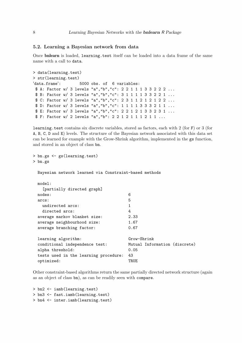
5.2. Learning a Bayesian network from data

Once bnlearn is loaded, learning.test itself can be loaded into a data frame of the samename with a call to data.

> data(learning.test)

> str(learning.test)

'data.frame': 5000 obs. of 6 variables:

$ A: Factor w/ 3 levels "a","b","c": 2 2 1 1 1 3 3 2 2 2 ...

$ B: Factor w/ 3 levels "a","b","c": 3 1 1 1 1 3 3 2 2 1 ...

$ C: Factor w/ 3 levels "a","b","c": 2 3 1 1 2 1 2 1 2 2 ...

$ D: Factor w/ 3 levels "a","b","c": 1 1 1 1 3 3 3 2 1 1 ...

$ E: Factor w/ 3 levels "a","b","c": 2 2 1 2 1 3 3 2 3 1 ...

$ F: Factor w/ 2 levels "a","b": 2 2 1 2 1 1 1 2 1 1 ...

learning.test contains six discrete variables, stored as factors, each with 2 (for F) or 3 (forA, B, C, D and E) levels. The structure of the Bayesian network associated with this data setcan be learned for example with the Grow-Shrink algorithm, implemented in the gs function,and stored in an object of class bn.

> bn.gs <- gs(learning.test)

> bn.gs

Bayesian network learned via Constraint-based methods

model:

[partially directed graph]

nodes: 6

arcs: 5

undirected arcs: 1

directed arcs: 4

average markov blanket size: 2.33

average neighbourhood size: 1.67

average branching factor: 0.67

learning algorithm: Grow-Shrink

conditional independence test: Mutual Information (discrete)

alpha threshold: 0.05

tests used in the learning procedure: 43

optimized: TRUE

Other constraint-based algorithms return the same partially directed network structure (againas an object of class bn), as can be readily seen with compare.

> bn2 <- iamb(learning.test)

> bn3 <- fast.iamb(learning.test)

> bn4 <- inter.iamb(learning.test)


> compare(bn.gs, bn2)

[1] TRUE


[1] TRUE


[1] TRUE

On the other hand hill-climbing results in a completely directed network, which differs fromthe previous one because the arc between A and B is directed (A→ B instead of A−B).

> bn.hc <- hc(learning.test, score = "aic")

> bn.hc

Bayesian network learned via Score-based methods

model:

[A][C][F][B|A][D|A:C][E|B:F]

nodes: 6

arcs: 5

undirected arcs: 0

directed arcs: 5




learning algorithm: Hill-Climbing

score: Akaike Information Criterion

penalization coefficient: 1

tests used in the learning procedure: 40

optimized: TRUE

> compare(bn.hc, bn.gs)

[1] FALSE

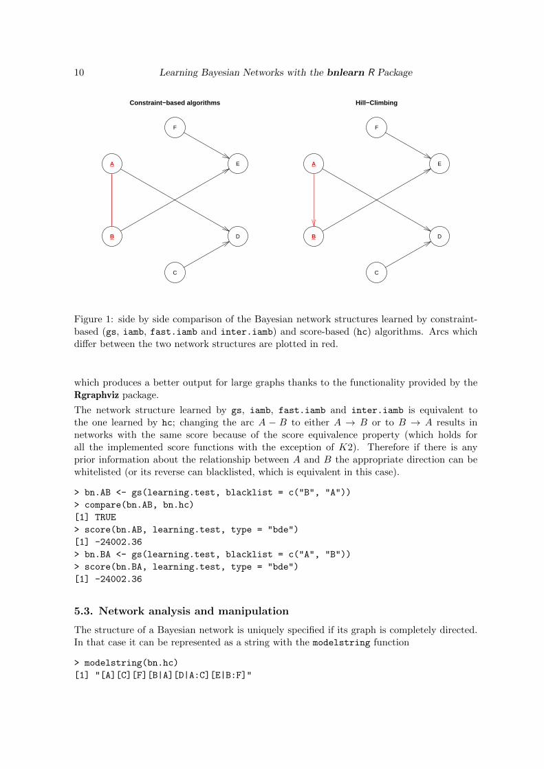
Another way to compare the two network structures is to plot them side by side and highlightthe differing arcs. This can be done either with the plot function (see Figure 1):

> par(mfrow = c(1,2))

> plot(bn.gs, main = "Constraint-based algorithms", highlight = c("A", "B"))

> plot(bn.hc, main = "Hill-Climbing", highlight = c("A", "B"))

or with the more versatile graphviz.plot:

> par(mfrow = c(1,2))

> highlight.opts <- list(nodes = c("A", "B"), arcs = c("A", "B"),

+ col = "red", fill = "grey")

> graphviz.plot(bn.hc, highlight = highlight.opts)

> graphviz.plot(bn.gs, highlight = highlight.opts)


Constraint−based algorithms

A

B

C

D

E

F

Hill−Climbing

A

B

C

D

E

F

Figure 1: side by side comparison of the Bayesian network structures learned by constraint-based (gs, iamb, fast.iamb and inter.iamb) and score-based (hc) algorithms. Arcs whichdiffer between the two network structures are plotted in red.

which produces a better output for large graphs thanks to the functionality provided by theRgraphviz package.

The network structure learned by gs, iamb, fast.iamb and inter.iamb is equivalent tothe one learned by hc; changing the arc A − B to either A → B or to B → A results innetworks with the same score because of the score equivalence property (which holds forall the implemented score functions with the exception of K2). Therefore if there is anyprior information about the relationship between A and B the appropriate direction can bewhitelisted (or its reverse can blacklisted, which is equivalent in this case).

> bn.AB <- gs(learning.test, blacklist = c("B", "A"))

> compare(bn.AB, bn.hc)

[1] TRUE

> score(bn.AB, learning.test, type = "bde")

[1] -24002.36

> bn.BA <- gs(learning.test, blacklist = c("A", "B"))

> score(bn.BA, learning.test, type = "bde")

[1] -24002.36

5.3. Network analysis and manipulation

The structure of a Bayesian network is uniquely specified if its graph is completely directed.In that case it can be represented as a string with the modelstring function

> modelstring(bn.hc)

[1] "[A][C][F][B|A][D|A:C][E|B:F]"


whose output is also included in the print method for the objects of class bn. Each nodeis printed in square brackets along with all its parents (which are reported after a pipe as acolon-separated list), and its position in the string depends on the partial ordering defined bythe network structure. The same syntax is used in deal (Boettcher and Dethlefsen 2003), anR package for learning Bayesian networks from mixed data.

Partially directed graphs can be transformed into completely directed ones with the set.arc,drop.arc and reverse.arc functions. For example the direction of the arc A − B in thebn.gs object can be set to A→ B, so that the resulting network structure is identical to theone learned by the hill-climbing algorithm.

> undirected.arcs(bn.gs)

from to

[1,] "A" "B"

[2,] "B" "A"

> bn.dag <- set.arc(bn.gs, "A", "B")

> modelstring(bn.dag)

[1] "[A][C][F][B|A][D|A:C][E|B:F]"

> compare(bn.dag, bn.hc)

[1] TRUE

Acyclicity is always preserved, as these commands return an error if the requested changeswould result in a cyclic graph.

> set.arc(bn.hc, "E", "A")

Error in arc.operations(x = x, from = from, to = to, op = "set",

check.cycles = check.cycles, :

the resulting graph contains cycles.

Further information on the network structure can be extracted from any bn object with thefollowing functions:

• whether the network structure is acyclic (acyclic) or completely directed (directed);

• the labels of the nodes (nodes), of the root nodes (root.nodes) and of the leaf nodes(leaf.nodes);

• the directed arcs (directed.arcs) of the network, the undirected ones (undirected.arcs)or both of them (arcs);

• the adjacency matrix (amat) and the number of parameters (nparams) associated withthe network structure;

• the parents (parents), children (children), Markov blanket (mb), and neighbourhood(nbr) of each node.

The arcs, amat and modelstring functions can also be used in combination with empty.graph

to create a bn object with a specific structure from scratch:

> other <- empty.graph(nodes = nodes(bn.hc))


> arcs(other) <- data.frame(

+ from = c("A", "A", "B", "D"),

+ to = c("E", "F", "C", "E"))

> other

Randomly generated Bayesian network

model:

[A][B][D][C|B][E|A:D][F|A]

nodes: 6

arcs: 4

undirected arcs: 0

directed arcs: 4




generation algorithm: Empty

This is particularly useful to compare different network structures for the same data, forexample to verify the goodness of fit of the learned network with respect to a particular scorefunction.

> score(other, data = learning.test, type = "aic")

[1] -28019.79

> score(bn.hc, data = learning.test, type = "aic")

[1] -23873.13

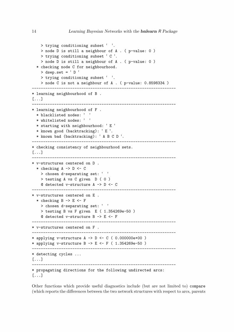
5.4. Debugging utilities and diagnostics

Many of the functions of the bnlearn package are able to print additional diagnostic messagesif called with the debug argument set to TRUE. This is especially useful to study the behaviourof the learning algorithms in specific settings and to investigate anomalies in their results(which may be due to an insufficient sample size for the asymptotic distribution of the teststo be valid, for example). For example the debugging output of the call to gs previously usedto produce the bn.gs object reports the exact sequence of conditional independence testsperformed by the learning algorithm, along with the effects of the backtracking optimizations(some parts are omitted for brevity).

> gs(learning.test, debug = TRUE)

----------------------------------------------------------------

* learning markov blanket of A .

* checking node B for inclusion.

> node B included in the markov blanket ( p-value: 0 ).

> markov blanket now is ' B '.* checking node C for inclusion.


> A indep. C given ' B ' ( p-value: 0.8743202 ).

* checking node D for inclusion.

> node D included in the markov blanket ( p-value: 0 ).

> markov blanket now is ' B D '.* checking node E for inclusion.

> A indep. E given ' B D ' ( p-value: 0.5193303 ).

* checking node F for inclusion.

> A indep. F given ' B D ' ( p-value: 0.07368042 ).

* checking node C for inclusion.

> node C included in the markov blanket ( p-value: 1.023194e-254 ).

> markov blanket now is ' B D C '.* checking node E for inclusion.

> A indep. E given ' B D C ' ( p-value: 0.5091863 ).

* checking node F for inclusion.

> A indep. F given ' B D C ' ( p-value: 0.3318902 ).

* checking node B for exclusion (shrinking phase).

> node B remains in the markov blanket. ( p-value: 9.224694e-291 )

* checking node D for exclusion (shrinking phase).

> node D remains in the markov blanket. ( p-value: 0 )

----------------------------------------------------------------

* learning markov blanket of B .

[...]

----------------------------------------------------------------

* learning markov blanket of F .

* known good (backtracking): ' B E '.* known bad (backtracking): ' A C D '.* nodes still to be tested for inclusion: ' '.

----------------------------------------------------------------

* checking consistency of markov blankets.

[...]

----------------------------------------------------------------

* learning neighbourhood of A .

* blacklisted nodes: ' '* whitelisted nodes: ' '* starting with neighbourhood: ' B D C '* checking node B for neighbourhood.

> dsep.set = ' E F '> trying conditioning subset ' '.> node B is still a neighbour of A . ( p-value: 0 )

> trying conditioning subset ' E '.> node B is still a neighbour of A . ( p-value: 0 )

> trying conditioning subset ' F '.> node B is still a neighbour of A . ( p-value: 0 )

> trying conditioning subset ' E F '.> node B is still a neighbour of A . ( p-value: 0 )

* checking node D for neighbourhood.

> dsep.set = ' C '


> trying conditioning subset ' '.> node D is still a neighbour of A . ( p-value: 0 )

> trying conditioning subset ' C '.> node D is still a neighbour of A . ( p-value: 0 )

* checking node C for neighbourhood.

> dsep.set = ' D '> trying conditioning subset ' '.> node C is not a neighbour of A . ( p-value: 0.8598334 )

----------------------------------------------------------------

* learning neighbourhood of B .

[...]

----------------------------------------------------------------

* learning neighbourhood of F .

* blacklisted nodes: ' '* whitelisted nodes: ' '* starting with neighbourhood: ' E '* known good (backtracking): ' E '.* known bad (backtracking): ' A B C D '.

----------------------------------------------------------------

* checking consistency of neighbourhood sets.

[...]

----------------------------------------------------------------

* v-structures centered on D .

* checking A -> D <- C

> chosen d-separating set: ' '> testing A vs C given D ( 0 )

@ detected v-structure A -> D <- C

----------------------------------------------------------------

* v-structures centered on E .

* checking B -> E <- F

> chosen d-separating set: ' '> testing B vs F given E ( 1.354269e-50 )

@ detected v-structure B -> E <- F

----------------------------------------------------------------

* v-structures centered on F .

----------------------------------------------------------------

* applying v-structure A -> D <- C ( 0.000000e+00 )

* applying v-structure B -> E <- F ( 1.354269e-50 )

----------------------------------------------------------------

* detecting cycles ...

[...]

----------------------------------------------------------------

* propagating directions for the following undirected arcs:

[...]

Other functions which provide useful diagnostics include (but are not limited to) compare

(which reports the differences between the two network structures with respect to arcs, parents


and children for each node), score and nparams (which report the number of parameters andthe contribution of each node to the network score, respectively).

6. Practical examples

6.1. The ALARM network

The ALARM (“A Logical Alarm Reduction Mechanism”) network from Beinlich et al. (1989)is a Bayesian network designed to provide an alarm message system for patient monitoring. Ithas been widely used (see for example Tsamardinos et al. (2006) and Friedman et al. (1999))as a case study to evaluate the performance of new structure learning algorithms.

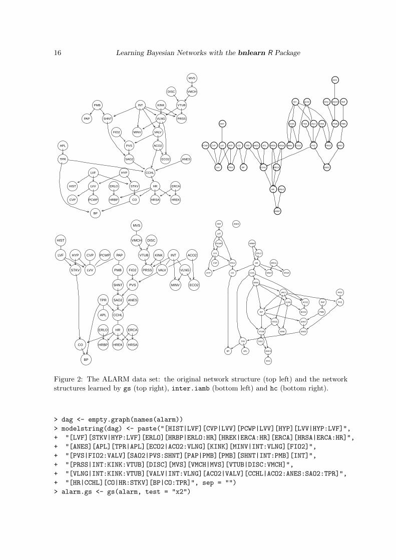
The alarm data set includes a sample of size 20000 generated from this network, whichcontains 37 discrete variables (with two to four levels each) and 46 arcs. Every learningalgorithm implemented in bnlearn (except mmpc) is capable of recovering the ALARM networkto within a few arcs and arc directions (see Figure 2).

> alarm.gs <- gs(alarm)

> alarm.iamb <- iamb(alarm)

> alarm.fast.iamb <- fast.iamb(alarm)

> alarm.inter.iamb <- inter.iamb(alarm)

> alarm.mmpc <- mmpc(alarm)

> alarm.hc <- hc(alarm, score = "bic")

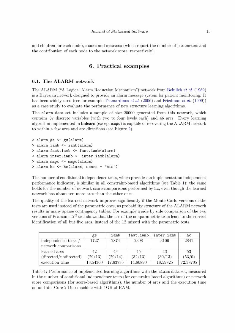
The number of conditional independence tests, which provides an implementation independentperformance indicator, is similar in all constraint-based algorithms (see Table 1); the sameholds for the number of network score comparisons performed by hc, even though the learnednetwork has about ten more arcs than the other ones.

The quality of the learned network improves significantly if the Monte Carlo versions of thetests are used instead of the parametric ones, as probability structure of the ALARM networkresults in many sparse contingency tables. For example a side by side comparison of the twoversions of Pearson’s X2 test shows that the use of the nonparametric tests leads to the correctidentification of all but five arcs, instead of the 12 missed with the parametric tests.

gs iamb fast.iamb inter.iamb hc

independence tests / 1727 2874 2398 3106 2841network comparisons

learned arcs 42 43 45 43 53(directed/undirected) (29/13) (29/14) (32/13) (30/13) (53/0)

execution time 13.54360 17.63735 14.80890 18.59825 72.38705

Table 1: Performance of implemented learning algorithms with the alarm data set, measuredin the number of conditional independence tests (for constraint-based algorithms) or networkscore comparisons (for score-based algorithms), the number of arcs and the execution timeon an Intel Core 2 Duo machine with 1GB of RAM.


ACO2

ANES

APL

BP

CCHL

COCVP

DISC

ECO2

ERCAERLO

FIO2

HIST HR

HRBP HREKHRSA

HYP

INT KINK

LVF

LVV

MINV

MVS

PAP

PCWP

PMB

PRSS

PVS

SAO2

SHNT

STKV

TPR

VALV

VLNG

VMCH

VTUB

●●

●

●

●

●

●

● ●

●

●

●

●●●

●

●● ●●

●

●

●

●

● ● ●

●●

●

●●

●

●● ●

●

CVPPCWP

HIST

TPR

BP

CO

HRBP

HREK HRSA

PAP

SAO2

FIO2

PRSSECO2MINV

MVS

HYPLVF APLANES

PMB

INT

KINK

DISC

LVV STKV CCHL

ERLOHR

ERCA

SHNTPVS

ACO2

VALVVLNG VTUB

VMCH

CVP PCWP

HIST

TPR

BP

CO HRBP HREK HRSA

PAP

SAO2

FIO2 PRSS

ECO2MINV

MVS

HYPLVF

APL

ANES

PMB

INTKINK

DISC

LVVSTKV

CCHL

ERLO HR ERCA

SHNT PVS

ACO2

VALV VLNG

VTUB

VMCH

CVP

PCWP

HIST

TPR

BP

CO

HRBP

HREK HRSA

PAP

SAO2

FIO2

PRSS

ECO2

MINV

MVS

HYP

LVF

APL

ANES

PMBINT

KINK

DISC

LVV

STKV

CCHL

ERLO

HR ERCA

SHNT

PVSACO2

VALV

VLNG

VTUB

VMCH

Figure 2: The ALARM data set: the original network structure (top left) and the networkstructures learned by gs (top right), inter.iamb (bottom left) and hc (bottom right).

> dag <- empty.graph(names(alarm))

> modelstring(dag) <- paste("[HIST|LVF][CVP|LVV][PCWP|LVV][HYP][LVV|HYP:LVF]",

+ "[LVF][STKV|HYP:LVF][ERLO][HRBP|ERLO:HR][HREK|ERCA:HR][ERCA][HRSA|ERCA:HR]",

+ "[ANES][APL][TPR|APL][ECO2|ACO2:VLNG][KINK][MINV|INT:VLNG][FIO2]",

+ "[PVS|FIO2:VALV][SAO2|PVS:SHNT][PAP|PMB][PMB][SHNT|INT:PMB][INT]",

+ "[PRSS|INT:KINK:VTUB][DISC][MVS][VMCH|MVS][VTUB|DISC:VMCH]",

+ "[VLNG|INT:KINK:VTUB][VALV|INT:VLNG][ACO2|VALV][CCHL|ACO2:ANES:SAO2:TPR]",

+ "[HR|CCHL][CO|HR:STKV][BP|CO:TPR]", sep = "")

> alarm.gs <- gs(alarm, test = "x2")


●●

●

●

●

●●

●

●

●●

●

● ●● ●●

●

● ●

●●

●

●

●

●

●●

●●

●

●

●

●●

●●

ACO2

ANES

APL

BP

CCHL

COCVP

DISC

ECO2

ERCAERLO

FIO2

HIST HR

HRBP HREKHRSA

HYP

INT KINK

LVF

LVV

MINV

MVS

PAP

PCWP

PMB

PRSS

PVS

SAO2

SHNT

STKV

TPR

VALV

VLNG

VMCH

VTUB

●●

●

●

●

●●

●

●

●●

●

● ●● ●●

●

● ●

●●

●

●

●

●

●●

●●

●

●

●

●●

●●

ACO2

ANES

APL

BP

CCHL

COCVP

DISC

ECO2

ERCAERLO

FIO2

HIST HR

HRBP HREKHRSA

HYP

INT KINK

LVF

LVV

MINV

MVS

PAP

PCWP

PMB

PRSS

PVS

SAO2

SHNT

STKV

TPR

VALV

VLNG

VMCH

VTUB

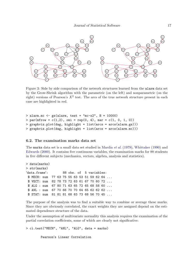
Figure 3: Side by side comparison of the network structures learned from the alarm data setby the Grow-Shrink algorithm with the parametric (on the left) and nonparametric (on theright) versions of Pearson’s X2 test. The arcs of the true network structure present in eachcase are highlighted in red.

> alarm.mc <- gs(alarm, test = "mc-x2", B = 10000)

> par(mfrow = c(1,2), omi = rep(0, 4), mar = c(1, 0, 1, 0))

> graphviz.plot(dag, highlight = list(arcs = arcs(alarm.gs)))

> graphviz.plot(dag, highlight = list(arcs = arcs(alarm.mc)))

6.2. The examination marks data set

The marks data set is a small data set studied in Mardia et al. (1979), Whittaker (1990) andEdwards (2000). It contains five continuous variables, the examination marks for 88 studentsin five different subjects (mechanics, vectors, algebra, analysis and statistics).

> data(marks)

> str(marks)

'data.frame': 88 obs. of 5 variables:

$ MECH: num 77 63 75 55 63 53 51 59 62 64 ...

$ VECT: num 82 78 73 72 63 61 67 70 60 72 ...

$ ALG : num 67 80 71 63 65 72 65 68 58 60 ...

$ ANL : num 67 70 66 70 70 64 65 62 62 62 ...

$ STAT: num 81 81 81 68 63 73 68 56 70 45 ...

The purpose of the analysis was to find a suitable way to combine or average these marks.Since they are obviously correlated, the exact weights they are assigned depend on the esti-mated dependence structure of the data.

Under the assumption of multivariate normality this analysis requires the examination of thepartial correlation coefficients, some of which are clearly not significative:

> ci.test("MECH", "ANL", "ALG", data = marks)

Pearson's Linear Correlation


MECH

VECT

ALG

ANL

STAT MECH

VECT

ALG

ANL

STAT

MECH

VECT

ALG

ANL

STAT

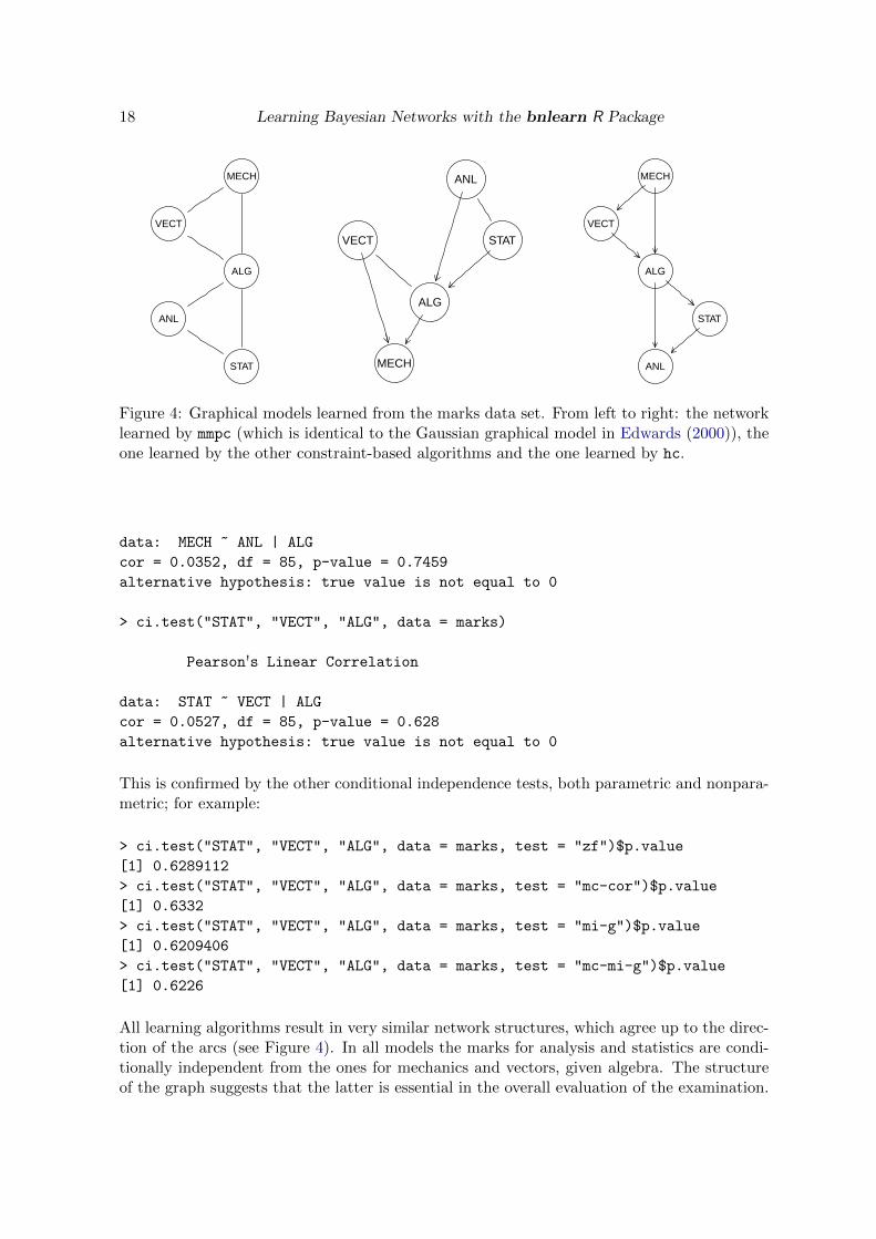
Figure 4: Graphical models learned from the marks data set. From left to right: the networklearned by mmpc (which is identical to the Gaussian graphical model in Edwards (2000)), theone learned by the other constraint-based algorithms and the one learned by hc.

data: MECH ~ ANL | ALG

cor = 0.0352, df = 85, p-value = 0.7459

alternative hypothesis: true value is not equal to 0

> ci.test("STAT", "VECT", "ALG", data = marks)

Pearson's Linear Correlation

data: STAT ~ VECT | ALG

cor = 0.0527, df = 85, p-value = 0.628

alternative hypothesis: true value is not equal to 0

This is confirmed by the other conditional independence tests, both parametric and nonpara-metric; for example:

> ci.test("STAT", "VECT", "ALG", data = marks, test = "zf")$p.value

[1] 0.6289112

> ci.test("STAT", "VECT", "ALG", data = marks, test = "mc-cor")$p.value

[1] 0.6332

> ci.test("STAT", "VECT", "ALG", data = marks, test = "mi-g")$p.value

[1] 0.6209406

> ci.test("STAT", "VECT", "ALG", data = marks, test = "mc-mi-g")$p.value

[1] 0.6226

All learning algorithms result in very similar network structures, which agree up to the direc-tion of the arcs (see Figure 4). In all models the marks for analysis and statistics are condi-tionally independent from the ones for mechanics and vectors, given algebra. The structureof the graph suggests that the latter is essential in the overall evaluation of the examination.


7. Other packages for learning Bayesian networks

There exist other packages in R which are able to either learn the structure of a Bayesian net-work or fit and manipulate its parameters. Some examples are pcalg, which implements thePC algorithm and focuses on the causal interpretation of Bayesian networks; deal, which im-plements a hill-climbing search for mixed data; and the suite composed by gRbase (Højsgaardet al. 2010), gRain (Højsgaard 2010), gRc (Højsgaard and Lauritzen 2008), which implementsvarious exact and approximate inference procedures.

However, none of these packages is as versatile as bnlearn for learning the structure of Bayesiannetworks. deal and pcalg implement a single learning algorithm, even though are able tohandle both discrete and continuous data. Furthermore, the PC algorithm has a poor perfor-mance in terms of speed and accuracy compared to newer constraint-based algorithms suchas Grow-Shrink and IAMB (Tsamardinos et al. 2003). bnlearn also offers a wider selectionof network scores and conditional independence tests; in particular it’s the only R packageable to learn the structure of Bayesian networks using permutation tests, which are superiorto the corresponding asymptotic tests at low sample sizes.

8. Conclusions

bnlearn is an R package which provides a free implementation of some Bayesian network struc-ture learning algorithms appeared in recent literature, enhanced with algorithmic optimiza-tions and support for parallel computing. Many score functions and conditional independencetests are provided for both independent use and the learning algorithms themselves.

bnlearn is designed to provide the versatility needed to handle experimental data analy-sis. It handles both discrete and continuous data, and it supports any combination of theimplemented learning algorithms and either network scores (for score-based algorithms) orconditional independence tests (for constraints-based algorithms). Furthermore, it simplifiesthe analysis of the learned networks by providing a single object class (bn) for all the al-gorithms and a set of utility functions to perform descriptive statistics and basic inferenceprocedures.

Acknowledgements

Many thanks to Prof. Adriana Brogini, my Supervisor at the Ph.D. School in StatisticalSciences (University of Padova), for proofreading this article and giving many useful commentsand suggestions. I would also like to thank Radhakrishnan Nagarajan (University of Arkansasfor Medical Sciences) and Suhaila Zainudin (Universiti Teknologi Malaysia) for their support,which encouraged me in the development of this package.

References

Acid S, de Campos LM, Fernandez-Luna J, Rodriguez S, Rodriguez J, Salcedo J (2004). “AComparison of Learning Algorithms for Bayesian Networks: A Case Study Based on Datafrom An Emergency Medical Service.” Artificial Intelligence in Medicine, 30, 215–232.


Bach FR, Jordan MI (2003). “Learning Graphical Models with Mercer Kernels.” In “Advancesin Neural Information Processing Systems (NIPS) 15,” pp. 1009–1016. MIT Press.

Beinlich I, Suermondt HJ, Chavez RM, Cooper GF (1989). “The ALARM Monitoring Sys-tem: A Case Study with Two Probabilistic Inference Techniques for Belief Networks.” In“Proceedings of the 2nd European Conference on Artificial Intelligence in Medicine,” pp.247–256. Springer-Verlag. URL http://www.cs.huji.ac.il/labs/compbio/Repository/

Datasets/alarm/alarm.htm.

Boettcher SG, Dethlefsen C (2003). “deal: A Package for Learning Bayesian Networks.” Jour-nal of Statistical Software, 8(20), 1–40. ISSN 1548-7660. URL http://www.jstatsoft.

org/v08/i20.

Chickering DM (1995). “A Transformational Characterization of Equivalent Bayesian NetworkStructures.” In “UAI ’95: Proceedings of the Eleventh Annual Conference on Uncertaintyin Artificial Intelligence,” pp. 87–98. Morgan Kaufmann.

Chickering DM (2002). “Optimal Structure Identification with Greedy Search.” Journal ofMachine Learning Research, 3, 507–554.

Cooper GF, Herskovits E (1992). “A Bayesian Method for the Induction of ProbabilisticNetworks from Data.” Machine Learning, 9(4), 309–347.

Daly R, Shen Q (2007). “Methods to Accelerate the Learning of Bayesian Network Structures.”In“Proceedings of the 2007 UK Workshop on Computational Intelligence,” Imperial College,London.

Edwards DI (2000). Introduction to Graphical Modelling. Springer.

Friedman N, Linial M, Nachman I (2000). “Using Bayesian Networks to Analyze ExpressionData.” Journal of Computational Biology, 7, 601–620.

Friedman N, Pe’er D, Nachman I (1999). “Learning Bayesian Network Structure from MassiveDatasets: The ”Sparse Candidate” Algorithm.” In “Proceedings of Fifteenth Conference onUncertainty in Artificial Intelligence (UAI),” pp. 206–221. Morgan Kaufmann.

Geiger D, Heckerman D (1994). “Learning Gaussian Networks.” Technical report, MicrosoftResearch, Redmond, Washington. Available as Technical Report MSR-TR-94-10.

Gentleman R, Whalen E, Huber W, Falcon S (2010). graph: A package to handle graph datastructures. R package version 1.26.0.

Gentry J, Long L, Gentleman R, Falcon S, Hahne F, Sarkar D (2010). Rgraphviz: ProvidesPlotting Capabilities for R Graph Objects. R package version 1.26.0.

Good P (2005). Permutation, Parametric and Bootstrap Tests of Hypotheses. Springer, 3rdedition.

Heckerman D, Geiger D, Chickering DM (1995). “Learning Bayesian Networks: The Combi-nation of Knowledge and Statistical Data.” Machine Learning, 20(3), 197–243. Availableas Technical Report MSR-TR-94-09.

http://www.cs.huji.ac.il/labs/compbio/Repository/Datasets/alarm/alarm.htm

http://www.cs.huji.ac.il/labs/compbio/Repository/Datasets/alarm/alarm.htm

http://www.jstatsoft.org/v08/i20

http://www.jstatsoft.org/v08/i20


Højsgaard S (2010). gRain: Graphical Independence Networks. R package version 0.8.5.

Højsgaard S, Dethlefsen C, Bowsher C (2010). gRbase: A package for graphical modelling inR. R package version 1.3.4.

Højsgaard S, Lauritzen SL (2008). gRc: Inference in Graphical Gaussian Models with Edgeand Vertex Symmetries. R package version 0.2.2.

Holmes DE, Jain LC (eds.) (2008). Innovations in Bayesian Networks: Theory and Applica-tions, volume 156 of Studies in Computational Intelligence. Springer.

Kalisch M, Buhlmann P (2007). “Estimating High-Dimensional Directed Acyclic Graphs withthe PC-Algorithm.” Journal of Machine Learning Research, 8, 613–66.

Korb K, Nicholson A (2004). Bayesian Artificial Intelligence. Chapman and Hall.

Kullback S (1959). Information Theory and Statistics. Wiley.

Lam W, Bacchus F (1994). “Learning Bayesian Belief Networks: An Approach Based on theMDL Principle.” Computational Intelligence, 10, 269–293.

Legendre P (2000). “Comparison of Permutation Methods for the Partial Correlation andPartial Mantel Tests.” Journal of Statistical Computation and Simulation, 67, 37–73.

Mardia KV, Kent JT, Bibby JM (1979). Multivariate Analysis. Academic Press.

Margaritis D (2003). Learning Bayesian Network Model Structure from Data. Ph.D. thesis,School of Computer Science, Carnegie-Mellon University, Pittsburgh, PA. Available asTechnical Report CMU-CS-03-153.

Moore A, Wong W (2003). “Optimal Reinsertion: A New Search Operator for Acceleratedand More Accurate Bayesian Network Structure Learning.” In “Proceedings of the 20thInternational Conference on Machine Learning (ICML ’03),” pp. 552–559. AAAI Press.

Neapolitan RE (2003). Learning Bayesian Networks. Prentice Hall.

Pearl J (1988). Probabilistic Reasoning in Intelligent Systems: Networks of Plausible Infer-ence. Morgan Kaufmann.

R Development Core Team (2009). R: A Language and Environment for Statistical Comput-ing. R Foundation for Statistical Computing, Vienna, Austria. ISBN 3-900051-07-0, URLhttp://www.R-project.org.

Rissanen J (1978). “Modeling by Shortest Data Description.” Automatica, 14, 465–471.

Spirtes P, Glymour C, Scheines R (2001). Causation, Prediction and Search. MIT Press.

Tierney L, Rossini AJ, Li N, Sevcikova H (2008). snow: Simple Network of Workstations. Rpackage version 0.3-3.

Tsamardinos I, Aliferis CF, Statnikov A (2003). “Algorithms for Large Scale Markov BlanketDiscovery.” In “Proceedings of the Sixteenth International Florida Artificial IntelligenceResearch Society Conference,” pp. 376–381. AAAI Press.

http://www.R-project.org


Tsamardinos I, Brown LE, Aliferis CF (2006). “The Max-Min Hill-Climbing Bayesian NetworkStructure Learning Algorithm.” Machine Learning, 65(1), 31–78.

Verma TS, Pearl J (1991). “Equivalence and Synthesis of Causal Models.” Uncertainty inArtificial Intelligence, 6, 255–268.

Whittaker J (1990). Graphical Models in Applied Multivariate Statistics. Wiley.

Witten IH, Frank E (2005). Data Mining: Practical Machine Learning Tools and Techniques.Morgan Kaufmann, 2nd edition.

Yaramakala S, Margaritis D (2005). “Speculative Markov Blanket Discovery for OptimalFeature Selection.” In “ICDM ’05: Proceedings of the Fifth IEEE International Conferenceon Data Mining,” pp. 809–812. IEEE Computer Society, Washington, DC, USA.

Affiliation:

Marco ScutariDepartment of Statistical SciencesUniversity of PadovaVia Cesare Battisti 241, 35121 Padova, ItalyE-mail: [email protected]

Journal of Statistical Software http://www.jstatsoft.org/

published by the American Statistical Association http://www.amstat.org/

Volume VV, Issue II Submitted: yyyy-mm-ddMMMMMM YYYY Accepted: yyyy-mm-dd

mailto:[email protected]

http://www.jstatsoft.org/

http://www.amstat.org/

Learning Bayesian Networks with the bnlearn R Package · 2 Learning Bayesian Networks with the...

Documents

Transcript of Learning Bayesian Networks with the bnlearn R Package · 2 Learning Bayesian Networks with the...