Learning-based inverse dynamics of human motion

Petrissa Zell and Bodo RosenhahnLeibniz University Hannover, Germany

zell@tnt.uni-hannover.de

Abstract

In this work we propose a learning-based algorithmfor the inverse dynamics problem of human motion. Ourmethod uses Random Forest regression to predict jointtorques and ground reaction forces from motion patterns.For this purpose we extend temporally incomplete forceplate data via a direct Random Forest regression from mo-tion parameters to force vectors. Based on the resultingcompleted data we estimate underlying joint torques using amodified physics-based predictive dynamics approach. Theoptimization results for model states and controls act aspredictors and responses for the final Random Forest re-gression from motion to joint torques and ground reactionforces.

The evaluation of our method includes a comparison tostate-of-the-art results and to measured force plate data anda demonstration of the robust performance under influenceof noisy and occluded input.

1. IntroductionThe analysis of human motion is indispensable for med-

ical applications, such as diagnostics and rehabilitation ofthe human locomotor system [10, 16, 17]. To measure theload at individual joints, researchers use the concept of jointtorques as the sum of all applied torques, e.g. caused bythe exerted forces of the skeleton, tendons and ligaments.Based on this concept the healthiness of human motion canbe assessed and abnormalities can be detected.

The biomechanical state of the art is to estimate jointtorques from motion data using optimization approaches. Aperformance measure, such as the dynamic effort, is mini-mized in compliance with a set of constraints. There existseveral different optimization formulations for this specificproblem, namely forward, inverse and predictive dynam-ics [3, 6, 21, 26, 27]. Characteristic challenges of thesemethods are high computational cost, non-convex param-eter spaces and large scale problems. Therefore these op-timization problems require a careful treatment regardinginitialisation and constraining in order to ensure conver-

Ground reaction force

& joint torques

3D motion states

Random Forest

regression

Figure 1. Random Forest regression from model states to con-trols. We consider short windows of three consecutive frames.The green arrows represent the ground reaction force and the redspheres are the joint torques.

gence. Furthermore the quality of the resulting joint torquesis strongly depending on the accuracy of the input joint po-sition trajectories which are generally obtained using a mo-tion capture system.

To address these issues we propose a learning-based ap-proach to estimate joint torques together with contact forcesfrom motion using a sliding window procedure coupledwith a Random Forest (RF) parameter regression. Since werely on learned correlations between motions and the in-ducing torques and forces our method is less susceptible tonoise and can even handle large occlusions (e.g. one entireleg).

A motion sequence is divided into overlapping windowswhich are separately fed to the RF to regress the underly-ing joint torques and contact forces, as illustrated in Fig. 1.Using a large window overlap we achieve smooth curve pro-gressions and since windows are processed seperately, ourmethod is suitable for parallelisation. Compared to the pre-dictive dynamics optimization, introduced in Sec. 3.2 wereduce computation times from over one hour to less thanthree minutes, on average (using unoptimized Matlab code).

In order to generate the RF we create a training set of

1

motion windows with optimized force and torque profilesbased on a physical model of the human body. The corre-sponding optimization problems are solved with a predic-tive dynamics approach [27]. In this context it is crucial toconstrain the modeled GRF and its point of action, the cen-ter of pressure (COP) since joint torques and contact forcesare interdependent.

We evaluate the performance of our method concerningcomputation time, GRF and COP estimation error and theconsistency of joint torques and compare with results gen-erated with a modified predictive dynamics approach andour own implementation of a state-of-the-art method byBrubaker et al. [7].

Our method generalizes to partly untrained and noisydata (cf. Sec. 4.2) and is independent of force plate measure-ments. In contrast to that, optimization-based approachesare often restricted to a laboratory setup or need careful con-straining to make up for the missing contact force measure-ments.

To summarize, we propose

• a learning-based approach for the inverse dynamicsproblem to estimate joint torques and contact forcesfrom motion.

• For this purpose, we introduce a Random Forestregression from motion to contact force properties(Force Regression Forest: FRF) to complete forceplate measurements (Sec. 3.2).

• Based on the completed data, we define contact reg-ularizations for a predictive dynamics optimization(PDO), that is used to generate training sets consistingof motion windows (Sec. 3.2).

• Finally, we regress joint torques and contact force vec-tors from motion parameters using a Random Foresttrained on the complete, regularized sets (Torque Re-gression Forest: TRF) (Sec. 3.3).

2. Related workPhysics-based modeling provides the basis for human

motion simulation and analysis in numerous state-of-the-art methods. Researchers in computer graphics use phys-ical models to synthesise realistically looking motions [2,12, 19, 24, 29]. The naturalness of an artificial motion caneither be achieved by exploiting motion capture data or byminimizing some kind of efficiency measure, e.g. the dy-namic effort. This approach is motivated by the overall ten-dency of humans to avoid energy expenditure.

In computer vision physical models are used to facilitatetasks like robust person and object tracking and 3D pose es-timation [6, 13, 14, 20, 15, 23, 25]. In [6] a simple planarmodel is exploited to estimate the biomechanical character-istics of gait and combined with a 3D kinematic model for

monocular tracking. A related approach by [23] considersnot only walking but a wide range of motion types. The au-thors propose a full-body 3D physical prior that integratesthe corresponding dynamics into a Bayesian filtering frame-work.

There are a number of recent methods that use physicalmodels and constraints to solve specific tasks of computervision: The works of Oikonomidis et al. [14] and Pham etal. [15] model hand-object interactions for hand pose track-ing and estimation of grasping forces, respectively. Maksaiet al. [13] and Park et al. [20] deal with the estimation ofouter forces effecting objects and persons in 2D images andvideos.

The works discussed so far use physical models to solvea specific problem but do not analyse the forces and torquesof a full human body model. The estimation of joint torquesfrom motion data is subject of human motion analysis andhas been realized by means of inverse dynamics [3, 26], for-ward dynamics [6] and predictive dynamics [21, 27]. All ofthese appoaches can be formulated as optimization prob-lems. In inverse dynamics, the model states, i.e. the motionparameters are set as optimization variables and the pro-ducing forces are calculated inversely from these states. Incontrast to that, forward dynamics treats the forces as opti-mization variables that generate a motion through integra-tion of the related equations of motion. Predictive dynamicsis closely related to Direct Collocation, known from opti-mal control problems: The states, as well as the forces areoptimized, while the equations of motion are incorporatedas equality constraints. General challenges of physics-basedoptimization are high computational expense concerningthe calculation of objectives, constraints and their deriva-tives and a high-dimensional parameter-space, resulting incomputation times in the order of hours.

Brubaker et al. address the issue of high computationalcost in [7]. They use an articulated body model to inferjoint torques and contact dynamics from 3D motion data.The optimization procedure is accelerated by introducingadditional root-forces which effectively decouple the equa-tions of motion at different time frames. These artificialroot-forces are then minimized.

In recent years, researchers aim to find a direct mappingfrom a motion parametrization to the acting forces, usingmachine learning techniques: [11] investigates sparse cod-ing for inverse dynamics regression via a CNN and [28] in-troduces a two dimensional statistical model for human gaitanalysis.

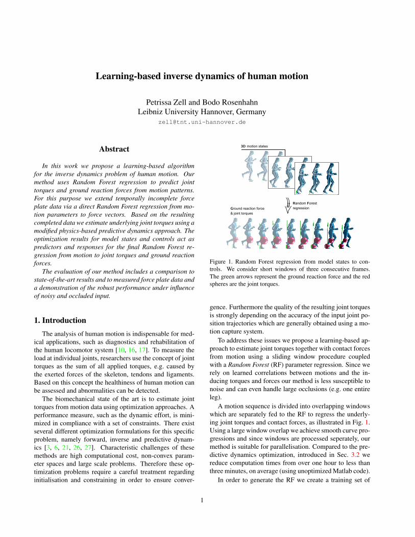
3. MethodThe proposed method relies on a training set that in-

cludes motion, GRF and joint torque parameters for shortoverlapping windows. In order to generate this set, the un-derlying joint torques and GRF have to be determined by

MoCap data: xmwith incompleteforce plate data:

Fm, r

states xmwith complete

Fm, r

DiReg(Sec. 3.2)

(c-)PDO(Sec. 3.2) training set: state

and controlparameters α, β

(c-)TRF(Sec. 3.3)

Regression result β→ GRF F ,

joint torques τ

Input:states x optimize

α

Data completionRegression

Figure 2. Flowchart of the proposed method.

means of a physics-based optimization procedure. In thiscontext the equations of motion of a physical model are usedas equality constraints. In the following section we will in-troduce the physical model and present the associated equa-tions of motion. A detailed description of the optimizationproblem follows in Sec. 3.2. To convey an overview of theproposed algorithm we depict a flowchart in Fig. 2.

3.1. Physical model

We use a physical model, consisting of 13 segments withrelated inertial properties, obtained from literature [9] and12 joints. The model has 29 degrees of freedom, that con-stitute the coordinates q. They comprise 6 global degreesof freedom for the position and the orientation of the rootjoint and 23 joint angles. The vector q is effected by thejoint torques τ with no actuation of the global coordinates,i.e. τ1, . . . , τ6 = 0.

For the modeling of the ground contact, the kinematicchain is equipped with two contact points for each foot seg-ment, one at the toe and one at the heel. The total GRF atone foot is distributed to both points, which enables us tosimulate a movement of the COP along the foot sole. Thisresults in the following contact force vector:

Fc = (fTcl1 ,fTcl2,fTcr1 ,f

Tcr2)T , (1)

which corresponds to stacked 3-dimensional force vectorsacting at the left toe, left heel, right toe and right heel. Theforce Fc is 12 dimensional and can be transformed fromR12×1 to R6×1 by a matrix C that adds the vectors actingat heel and toe:

F = CFc =

(fcl1 + fcl2fcr1 + fcr2

)=

(fclfcr

). (2)

The equations of motion are formulated using a combi-nation of the Newton-Euler method and the Lagrange for-malism, in general referred to as TMT-method [18]. Theyhave the following form:

Mq = τ + JTM(ag −G) + JTc Fc , (3)

with inertia matrices M and M(q) = J(q)TMJ(q) fordependent and independent coordinates, respectively. Thekinematics of the corresponding coordinate transformationare described by the Jacobian J(q) and the contact Jaco-bian Jc(q). Finally, ag and G(q, q) = ∂

∂q (J(q)q)q aregravitational and convective acceleration, respectively. Weshorten the right hand side of Eq. (3) by Mq = F(x,u),with the parameter sets

x = (qT , qT )T and u = (τT ,F Tc )T , (4)

called model states and controls, respectively.

3.2. Generation of training data

We decompose a sequence into windows of 3 frameswith an overlap of 2 frames. This window length yields suf-ficient information to reflect the acceleration of the modelstates, while allowing the use of 2nd order Hermite poly-nomials for the state and control discretization. The largeoverlap is necessary to facilitate a highly resolved analysisof motion sequences and to generate a maximal training set.

Predictive dynamics

For every motion window (discretized on the temporal gridt = t1, ..., t3) we estimate the underlying joint torques andGRF, i.e. we determine the control vector u that generatesthe considered motion using an optimization approach. Toreduce the number of design variables, the model states xand the control parameters u are descretized by approxi-mating them with Hermite polynomials Hi(t):

x(t) =

2∑i=1

αiHi(t) , u(t) =

2∑i=1

βiHi(t) (5)

The weighting coefficients α and β become optimizationparameters of a predictive dynamics approach [27] and willlater be used for the RF regression. They are optimized si-multaneously in compliance with a set of constraints. Thisset typically encompasses constraints for the motion pat-tern, the contact dynamics and in particular for the equa-tions of motion, which have to be fulfilled at the temporalgrid points. Due to measurement inaccuracies and modelsimplifications it is sometimes difficult to find a valid setfor these constraints.

Modified predictive dynamics

We phrase the predictive dynamics optimization using reg-ularization terms, introduced in Eq. (7) instead of hard con-straints to support the convergence. The problem

minαβ

{w0hτ (β) + w1he(α,β) (6)

+w2hx(α) + w3hf(β) + w4hd(β)},

is solved using an interior point algorithm [8]. Here,w0, . . . , w4 > 0 are weighting factors that sum to one.

The individual terms of Eq. (6) are defined as follows:

hτ (β) =1

T

∑i

‖τ (ti)‖2 (7a)

he(α,β) =1

T

∑i

‖Mq(ti)−F(x(ti),u(ti))‖2 (7b)

hx(α) =1

T

∑i

‖x(ti)− xm(ti)‖2 (7c)

hf(β) =1

T

∑i

‖F (ti)− Fm(ti)‖2 (7d)

hd(β) =1

T

∑i

∑j=l,r

((‖fcj1(ti)‖ − rj2(ti)‖fcj (ti)‖

)2+(‖fcj2(ti)‖ − rj1(ti)‖fcj (ti)‖

)2)(7e)

with the duration T = t3 − t1 of 3 frames.The first term hτ is the so called dynamic effort, which

penalizes large joint torques. The second function he de-scribes the violation of the equations of motion, defined inEq. (3). Furthermore we minimize the terms hx and hfto prevent a strong deviation of the states and the modeledGRF from ground truth values. Here, measured data is in-dicated by an index m. In particular, xm are the states ofa model, fitted directly to the captured joint trajectories andFm is based on the measured force plate data but temporallyextended using a RF regression that will be described in thenext section.

Finally in Eq. (7e), we regularize the force partitioningbetween toe and heel contact points depending on the re-spective distances of these points to the COP on the forceplate, i.e. to the point of action of the GRF vector. Moreprecisely, we enforce a linear distribution of force vectorsaccording to the relative distances

r = (rl1, rl2, rr1, rr2)T =

( 1dl1+dl2

(dl1, dl2)T

1dr1+dr2

(dr1, dr2)T

). (8)

Here, (dl1, dl2, dr1, dr2) denote the distances of the lefttoe, left heel, right toe and right heel to the COP.

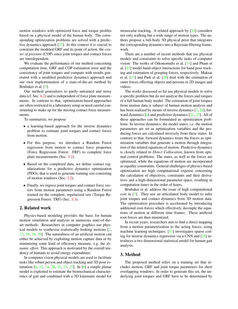
To demonstrate the influence of hd, we compare the sim-ulated COP motion during the stance phase of walking withand without its minimization and analyze the resulting an-kle torque profiles: The left side of Fig. 3 shows the op-timized relative force magnitude ‖fcl1‖/‖fcl‖ at the toecontact point compared to the ground truth distance rl2.Without regularization the resulting force partitioning canonly approximate the COP position during mid-stance, butfails shortly after and before heel-strike and toe-off, respec-tively. Based on such a contact force distribution the ankle

0.5 0.6 0.7 0.8 0.9 1time [s]

0

0.2

0.4

0.6

0.8

1

1.2

rela

tive

forc

e (d

ista

nce)

|fcl1|/|fcl||fcl1|/|fcl |

Ground truth rl2

c-PDOPDO

0 20 40 60 80 100% gait cycle

-0.2

0

0.2

0.4

0.6

0.8

1

1.2

ankl

e to

rque

[Nm

/kg]

weights w (c-PDO)

(PDO)weights waweights wb

Figure 3. Left: Comparison of optimized relative forces at the toeto the measured relative heel-to-COP distance rl2. Right: Influ-ence of different weight vectors on the optimized ankle torque.The vectors wb (PDO) and w (c-PDO) set hd and hτ to zero, re-spectively.

torque significantly differs from the optimization result withinclusion of hd, as can be seen in Fig. 3 on the right side.The figure shows optimized ankle torques resulting with theregularization weightsw = (0, 0.249, 0.249, 0.499, 0.003),wa = (0.024, 0.243, 0.243, 0.487, 0.003) and wb =(0.024, 0.244, 0.244, 0.488, 0). With wb (hd set to zero),an unrealistically high plantar flexion moment is necessaryto reach foot-flat and a dorsi flexion moment appears at toe-off to avoid hyperextension.

The optimization with regularization weightsw does nottake hτ (cf. Eq. (7a)) into consideration. An additional min-imization of this term, i.e. using the weights wa, does notchange the characteristic torque progression, while in turnincreasing the other regularization terms, e.g. the violationof the equations of motion he. In the following we will referto the window-wise predictive dynamics optimization withregularization according to w as COP-regularized predic-tive dynamics optimization (c-PDO) and to the correspond-ing procedure with wb as PDO.

Data completion

We recorded motion sequences of walking, jogging andjumping subjects in a laboratory setup with two force platesembedded in the ground to measure Fm. For walking andjogging the captured force plate data does not represent awhole cycle in many cases, since the subjects only hit oneplate to maintain a natural movement style.

Because the quality of the final torque regression corre-lates to the size of the training set, i.e. the number of mo-tion windows, we decided to complete the partial force platedata with inferred GRF values. This regression is termedas Force Regression Forest (FRF) and is realized using abagged Random Forest [4] that is trained with the predictormatrix AFRF and the response matrix BFRF. These matri-ces consist of parameter vectors for all N frames of motion

capture data of each motion class:

AFRF =

q1 . . . qNyc1 . . .ycNvc1 . . .vcN

, BFRF =

(Fm1

. . .FmN

r1 . . . rN

)(9)

We infer GRF vectors Fm and relative contact point toCOP distances r from the angular accelerations q, the verti-cal distances yc of the contact points to the ground and theirvelocities vc. Here, q is calculated using finite differencesof three consecutive frames. The contact parameters yc andvc are computed based on the model state of the respectivecenter frame. In our experience, a regression based on thesefeatures instead of the joint trajectories or the model statesprovides better results for this particular problem.

3.3. Joint torque and force regression

The RF regression described in the previous section pro-vides completed force plate data Fm and r which is thenused in Eq. (7d) and (7e) to regulate the contact force andits point of action during the optimization of the coefficientsα and β. These weighting coefficients determine the quan-tities of interest, that is the GRF F (t) and the joint torquesτ (t).

In other words, the successive execution of the forceregression FRF and the predictive dynamics optimization(c-)PDO provides training sets for the final RF regressionfrom motion to hidden forces and torques. These train-ing sets include parameter vectors α and β for the statesx = (qT , qT )T and the controls u = (τT ,F Tc )T , re-spectively. The final RF regression from motion to torquesand forces will be referred to as Torque Regression Forest(TRF) in the remainder of the paper. The whole algorithmis schematically presented in Fig. 2. We introduce the nota-tions TRF and c-TRF to distinguish between the RF trainedwith the parameters resulting from PDO and c-PDO, respec-tively.

To support the consideration of parameter correlationswe first perform principle component analysis on both thepredictor and the response set and then train a RF on theresulting principle component scores. We use a bagged RF[4] comprising 110 decision trees with a minimal leaf sizeof 3 parameter vectors. These properties were determinedvia cross validation. The forest is trained using the predictorvaluesATRF and the responsesBTRF consisting of princi-ple component scores s:

ATRF =(sin1 . . . s

inK

), BTRF =

(sout1 . . . soutK

), (10)

sin = C−1in (θ − θ) , sout = C−1

out(β − β) .

Here, Cin and Cout denote the corresponding principlecomponents and the mean of a variable is marked with ahorizontal bar above the character. The integer K is the

number of motion windows in the training set. The predic-tor scores are based on the parameter vector

θ = (αTr , qT ,vTc )T . (11)

The angular acceleration q is calculated via finite differ-ences and the contact point velocities vc are derived fromthe states x(t) and averaged over the window length. Asalready stated in Sec. 3.2, we found that these additionalfeatures improve the performance of the regression.

Instead of the complete coefficient vectorα, we use a re-duced version αr that does not include the coefficients forthe global position of the root joint. Thereby, we achievetranslational invariance of the predictors. Based on the re-sponse score sout we calculate β and subsequently the jointtorques τ and the GRF F via Eq. (2), (4) and (5).

For the application of (c-)TRF the considered motion se-quence first has to be divided into windows of 3 frames,with possible overlap. Then every window can be processedindependently making the algorithm suitable for paralleliza-tion. We determine the coefficients α by solving the iso-lated optimization problem min

α{hx(α)} (cf. Eq. (7c)) us-

ing the BFGS Quasi-Newton method [5] and subsequentlyreduce to αr. The remaining parameters q and vc fromEq. (11) are derived as described above.

4. ExperimentsWe use synchronized motion capture and force plate data

of 11 subjects that perform walking, jogging and verticaljumping motions. In total our training sets consist of 38sequences for each, walking and jogging and 36 sequencesfor jumping.

We obtain the 3D motion using a marker-based ViconT-series motion capture system consisting of 8 IR-camerasand measure the related GRF with AMTI force plates.Based on 3D marker trajectories a skeleton fit is performedand the resulting joint trajectories are used to calculate jointangles, angular velocities, root position and root velocity,which constitute the model states x(t) (cf. Eq. 4).

4.1. Data completion

First of all we will evaluate FRF that we use to com-plete force plate data for walking and jogging motions(cf. Sec. 3.2). As mentioned earlier, the resulting GRFvalues are used as regularization during the window-wisepredictive dynamics optimization and their quality is criti-cal for a sound joint torque estimation. Therefore we useall available information, including frames of the same se-quence that have valid GRF measurements.

For the evaluation of FRF we consider each motion se-quence separately and regress forces based on all remain-ing sequences in the set, hence using data from the samesubject as well. The mean square error (MSE) of inferred

0 0.2 0.4 0.6time [s]

0

5

10

15

20

GR

F [N

/kg]

0 0.2 0.4 0.6 0.8 1time [s]

0

5

10

15

GR

F [N

/kg]

FRF leftFRF rightForce plate leftForce plate right

Figure 4. Qualitative comparison of FRF results for the ver-tical GRF to force plate data of walking (left) and jogging(right). The sequences have MSE values of 0.091 (N/kg)2 and0.991 (N/kg)2, respectively.

GRF compared to ground truth data is used as error mea-sure. We achieve MSE values of 0.085 (N/kg)2 for walkingand 1.017 (N/kg)2 for jogging. Corresponding results arequalitatively compared to force plate data in Fig. 4. The lefthand side shows the vertical force for walking and the righthand side depicts the equivalent component for jogging. Welimit the qualitative presentation of results to vertical com-ponents, since they predominantly influence the dynamicsof the model. The quality of regressed horizontal compo-nents is similar and they are included in the MSE as well.

Note that in this particular jogging sequence the rightfoot does not hit the force plate. Therefore the measuredforce is equal to zero and does not represent the true GRF.In this case, our regression can be used for data completion.

Aside from the GRF vectors we need the relative dis-tances of toe and heel contact points to the COP on the forceplate, to ensure a realistic force partitioning during the op-timization. The MSE of the relative distances r is 0.012 forwalking and 0.011 for jogging.

This part of the evaluation does not consider the verticaljumps, since the subjects were able to hit both force platesduring jump and landing, providing us with complete forceplate data.

4.2. Joint torque and force estimation

In this section we evaluate the results of TRF and c-TRF(cf. Sec. 3.3), i.e. the estimated GRFs and joint torques. Weassess the performance of the regression forests by compar-ing to our own implementation of [7] and to the optimiza-tion procedures PDO and c-PDO introduced in Sec. 3.2.The quantitative evaluation will include the MSE of GRFand partitioned GRF magnitudes according to the COP, aswell as a comparison of computation times tc. Since thereis no ground truth data for joint torques we will analyze theconsistency of the resulting curves. In contrast to the evalu-ation of FRF, all motions performed by the same subject asthe considered motion sequence are now excluded from thetraining set.

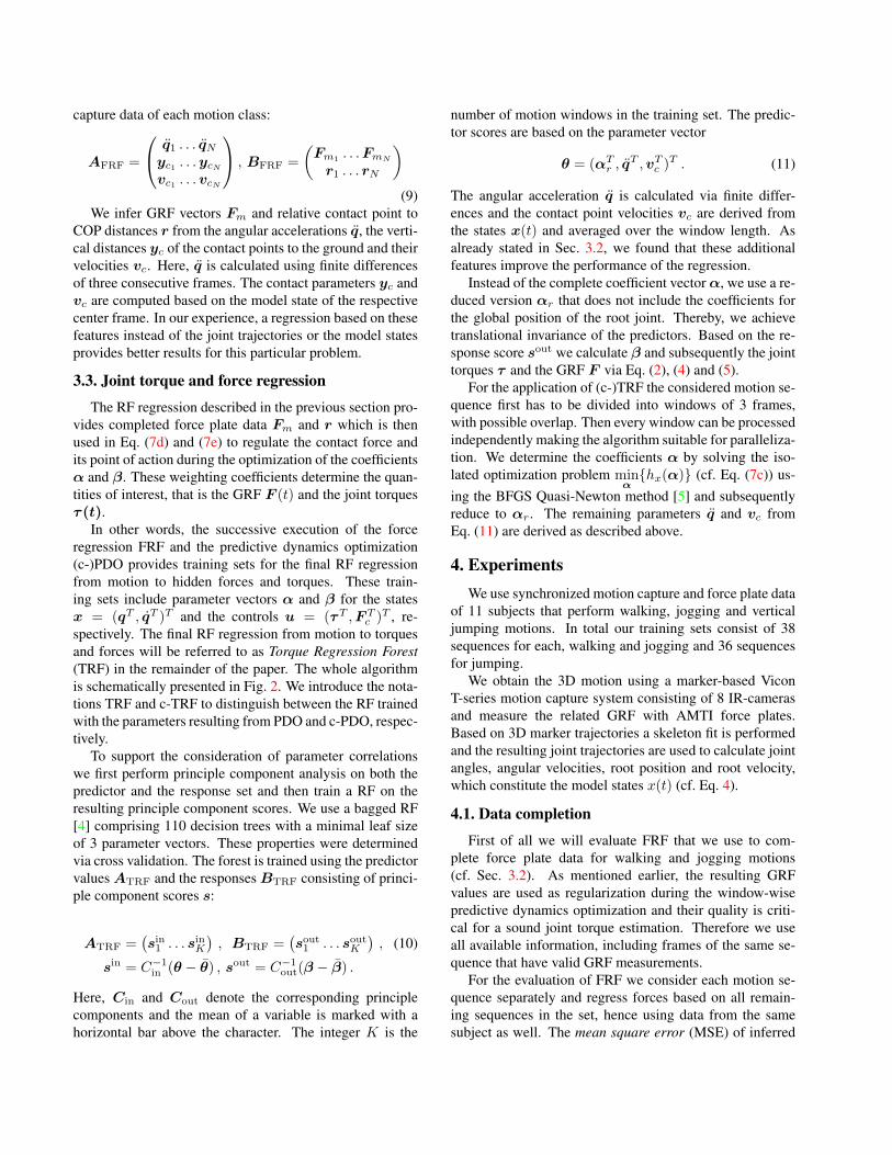
The left of Fig. 5 shows GRF regression results for exam-

ple sequences of all motion types. The corresponding MSEvalues and computation times for all sequences are summa-rized in Table 1. The window-wise predictive dynamics op-timization (c-)PDO clearly outperforms the method basedon [7] regarding MSE of GRF and COP for all motion types.But it suffers from high computation times (> 1h). Toachieve a faster estimation with relatively small error val-ues, c-TRF is the method of choice. In contrast to [7], itis able to estimate characteristic features, such as the dropof vertical GRF values during mid-stance of walking. Fur-thermore the vertical GRF component stays close to zeroduring the swing phase (no ground contact of the consid-ered foot) of walking and jogging, while the results of [7]considerably deviate from zero (cf. Fig 5). This discrepancyis due to the sensitivity of the latter method to the distanceof contact points to the estimated ground plane.

The COP MSE values demonstrate the effect of our COPregularization on the force partitioning between heel and toecontact points. The values are considerably decreased fromPDO to c-PDO and from TRF to c-TRF, respectively. Apartfrom the limiting of the GRF vector, this regularization iscrucial to ensure accurately estimated joint torques. It isnoteworthy, that the averaging of the RF regression tends toimprove the COP MSE of TRF compared to PDO.

For jogging and jumping, the performances of (c-)TRFand [7] are more similar than for walking. This can be ex-plained by the higher variability of these motion types, thatis not sufficiently reflected by the training sets. In order tosatisfy the higher variability it is advisable to increase thenumber of training samples for these motion types to fur-ther improve the results in future research.

To convey a qualitative impression of the performanceon the whole sets, we illustrate the mean and standard de-viation of the estimated vertical GRF via c-TRF and [7] inFig. 5 on the left. The corresponding curves for the jointtorques inferred with c-TRF are shown in Fig. 5 on theright. The torque profiles display a high degree of consis-tency (small standard deviations) for walking and jogging.In the case of jumping the results are affected by a higheruncertainty concerning the distinction between jump, flightand landing phase, which is reflected in the non-zero GRFduring the flight phase. This problem could be approachedby employing an additional classification previous to the RFregression, i.e. with a hierarchical RF or by simply increas-ing the training set. Nevertheless, the MSE values for GRFand COP are lower than those achieved with [7].

4.3. Noise and occlusions

In order to demonstrate the robustness of our method weevaluate the performance on noisy and occluded data. In afirst experiment we add gaussian noise to the coordinates qof the walking sequences and analyze the resulting MSEof the inferred GRF (cf. Fig. 6 left). The regression for

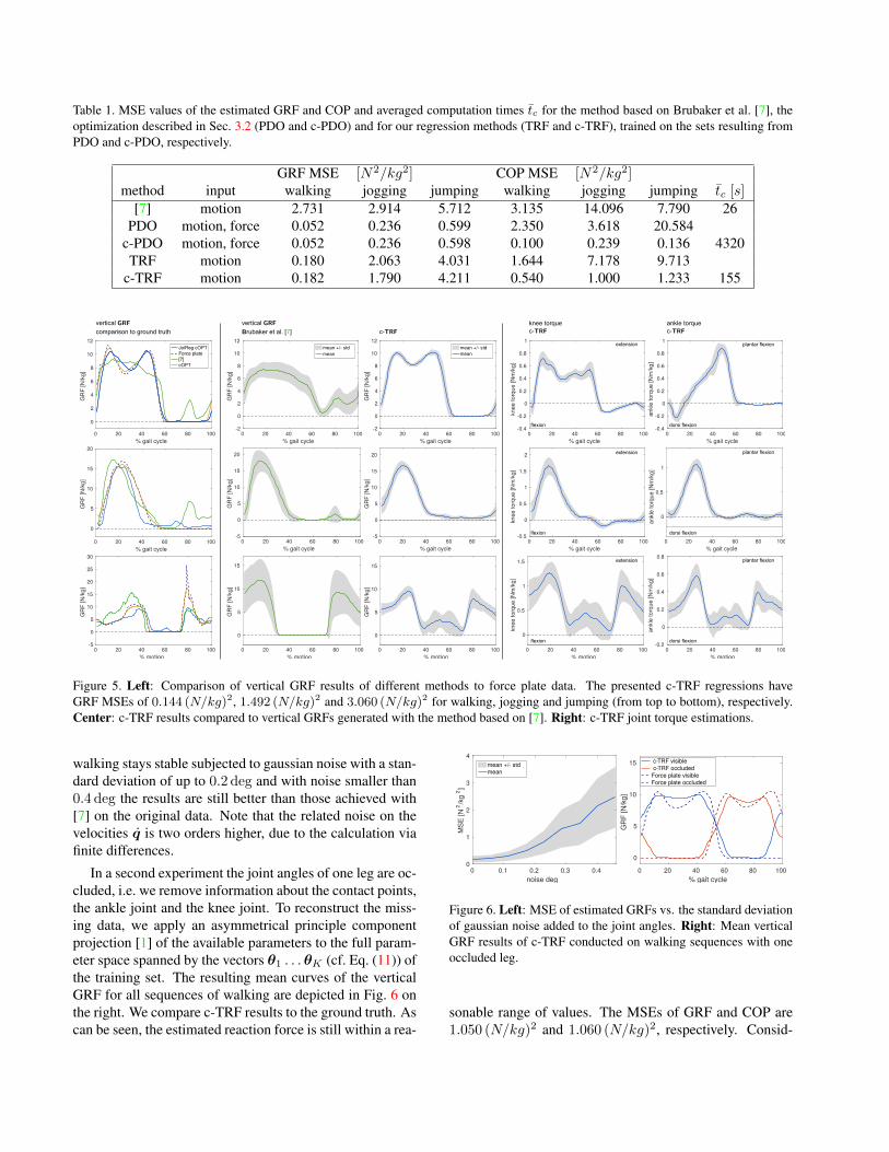
Table 1. MSE values of the estimated GRF and COP and averaged computation times tc for the method based on Brubaker et al. [7], theoptimization described in Sec. 3.2 (PDO and c-PDO) and for our regression methods (TRF and c-TRF), trained on the sets resulting fromPDO and c-PDO, respectively.

GRF MSE [N2/kg2] COP MSE [N2/kg2]method input walking jogging jumping walking jogging jumping tc [s]

[7] motion 2.731 2.914 5.712 3.135 14.096 7.790 26PDO motion, force 0.052 0.236 0.599 2.350 3.618 20.584

c-PDO motion, force 0.052 0.236 0.598 0.100 0.239 0.136 4320TRF motion 0.180 2.063 4.031 1.644 7.178 9.713

c-TRF motion 0.182 1.790 4.211 0.540 1.000 1.233 155

0 20 40 60 80 100% gait cycle

-0.5

0

0.5

1

1.5

2

knee

torq

ue [N

m/k

g]

0 20 40 60 80 100% gait cycle

-0.4

-0.2

0

0.2

0.4

0.6

0.8

1

knee

torq

ue [N

m/k

g]

extension

extension

0 20 40 60 80 100% motion

0

0.5

1

1.5

knee

torq

ue [N

m/k

g]

extension

flexion

flexion

flexion

0 20 40 60 80 100% gait cycle

-0.4

-0.2

0

0.2

0.4

0.6

0.8

1

ankl

e to

rque

[Nm

/kg]

plantar flexion

0 20 40 60 80 100% gait cycle

0

0.5

1

ankl

e to

rque

[Nm

/kg]

plantar flexion

0 20 40 60 80 100% motion

-0.2

0

0.2

0.4

0.6

0.8

ankl

e to

rque

[Nm

/kg]

plantar flexion

dorsi flexion

dorsi flexion

dorsi flexion

0 20 40 60 80 100% gait cycle

-2

0

2

4

6

8

10

12

GR

F [N

/kg]

mean +/- stdmean

0 20 40 60 80 100% gait cycle

-5

0

5

10

15

20

GR

F [N

/kg]

0 20 40 60 80 100% gait cycle

-2

0

2

4

6

8

10

12

GR

F [N

/kg]

mean +/- stdmean

0 20 40 60 80 100% gait cycle

-5

0

5

10

15

20

GR

F [N

/kg]

0 20 40 60 80 100% motion

0

5

10

15

GR

F [N

/kg]

0 20 40 60 80 100% motion

0

5

10

15

GR

F [N

/kg]

vertical GRF

Brubaker et al. [7] c-TRF

0 20 40 60 80 100% gait cycle

0

2

4

6

8

10

12

GR

F [N

/kg]

JoiReg cOPTForce plate[7]cOPT

0 20 40 60 80 100% gait cycle

0

5

10

15

20

GR

F [N

/kg]

0 20 40 60 80 100% motion

-5

0

5

10

15

20

25

30

GR

F [N

/kg]

vertical GRF

comparison to ground truthknee torquec-TRF

ankle torquec-TRF

Figure 5. Left: Comparison of vertical GRF results of different methods to force plate data. The presented c-TRF regressions haveGRF MSEs of 0.144 (N/kg)2, 1.492 (N/kg)2 and 3.060 (N/kg)2 for walking, jogging and jumping (from top to bottom), respectively.Center: c-TRF results compared to vertical GRFs generated with the method based on [7]. Right: c-TRF joint torque estimations.

walking stays stable subjected to gaussian noise with a stan-dard deviation of up to 0.2 deg and with noise smaller than0.4 deg the results are still better than those achieved with[7] on the original data. Note that the related noise on thevelocities q is two orders higher, due to the calculation viafinite differences.

In a second experiment the joint angles of one leg are oc-cluded, i.e. we remove information about the contact points,the ankle joint and the knee joint. To reconstruct the miss-ing data, we apply an asymmetrical principle componentprojection [1] of the available parameters to the full param-eter space spanned by the vectors θ1 . . .θK (cf. Eq. (11)) ofthe training set. The resulting mean curves of the verticalGRF for all sequences of walking are depicted in Fig. 6 onthe right. We compare c-TRF results to the ground truth. Ascan be seen, the estimated reaction force is still within a rea-

0 20 40 60 80 100% gait cycle

0

5

10

15

GR

F [N

/kg]

Force plate visibleForce plate occluded

c-TRF visiblec-TRF occluded

0 0.1 0.2 0.3 0.4noise deg

0

1

2

3

4

MSE

[N2 /k

g2 ]

mean +/- stdmean

Figure 6. Left: MSE of estimated GRFs vs. the standard deviationof gaussian noise added to the joint angles. Right: Mean verticalGRF results of c-TRF conducted on walking sequences with oneoccluded leg.

sonable range of values. The MSEs of GRF and COP are1.050 (N/kg)2 and 1.060 (N/kg)2, respectively. Consid-

0 0.5 1time [s]

0

5

10

15

GR

F [N

/kg]

leftright

0 0.5 1 1.5 2time [s]

-0.2

0

0.2

0.4

0.6

0.8

1

ankl

e to

rque

[Nm

/kg]

healthyunhealthy

Figure 7. Left: Regressed vertical GRF for a transition from walk-ing to jogging (cf. Fig. 8). Right: Ankle torques of an asymmetricgait (cf. Fig. 9).

ering the plateau-like curve progression, we can concludethat especially the uncertainty in regressed event times, i.e.heel-strike, foot-flat, heel-off and toe-off is increased com-pared to regressions on the full information. Note that themeasured force on one plate is equal to zero during the firstand third double support, since our laboratory setup onlyconsists of two plates. The true GRF has to be greater thanzero like the regression results.

4.4. Application to new motions

The division into short windows allows us to infer forcesand torques of motions that are not part of the training set.The considered motion types are a transition from walkingto jogging and an asymmetric gait. On the level of 3-framewindows both sequences have some similarity to the learnedmotion classes, making a regression possible.

First, we consider the transition from walking to jogging.For this purpose we train a RF on the combined training setof walking and jogging sequences and perform the sameregression as before. In doing so, we rely on the capacityof c-TRF to automatically distinguish between both motiontypes. The resulting vertical GRF is illustrated in Fig. 7on the left hand side and frames from the correspondinganimation are shown in Fig. 8.

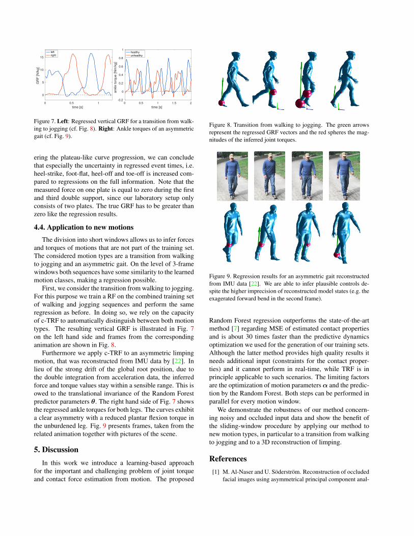
Furthermore we apply c-TRF to an asymmetric limpingmotion, that was reconstructed from IMU data by [22]. Inlieu of the strong drift of the global root position, due tothe double integration from acceleration data, the inferredforce and torque values stay within a sensible range. This isowed to the translational invariance of the Random Forestpredictor parameters θ. The right hand side of Fig. 7 showsthe regressed ankle torques for both legs. The curves exhibita clear asymmetry with a reduced plantar flexion torque inthe unburdened leg. Fig. 9 presents frames, taken from therelated animation together with pictures of the scene.

5. DiscussionIn this work we introduce a learning-based approach

for the important and challenging problem of joint torqueand contact force estimation from motion. The proposed

Figure 8. Transition from walking to jogging. The green arrowsrepresent the regressed GRF vectors and the red spheres the mag-nitudes of the inferred joint torques.

Figure 9. Regression results for an asymmetric gait reconstructedfrom IMU data [22]. We are able to infer plausible controls de-spite the higher imprecision of reconstructed model states (e.g. theexagerated forward bend in the second frame).

Random Forest regression outperforms the state-of-the-artmethod [7] regarding MSE of estimated contact propertiesand is about 30 times faster than the predictive dynamicsoptimization we used for the generation of our training sets.Although the latter method provides high quality results itneeds additional input (constraints for the contact proper-ties) and it cannot perform in real-time, while TRF is inprinciple applicable to such scenarios. The limiting factorsare the optimization of motion parametersα and the predic-tion by the Random Forest. Both steps can be performed inparallel for every motion window.

We demonstrate the robustness of our method concern-ing noisy and occluded input data and show the benefit ofthe sliding-window procedure by applying our method tonew motion types, in particular to a transition from walkingto jogging and to a 3D reconstruction of limping.

References[1] M. Al-Naser and U. Soderstrom. Reconstruction of occluded

facial images using asymmetrical principal component anal-

ysis. Integrated Computer-Aided Engineering, 19(3):273–283, 2012. 7

[2] S. Andrews, I. Huerta, T. Komura, L. Sigal, and K. Mitchell.Real-time physics-based motion capture with sparse sensors.In Proceedings of the 13th European Conference on VisualMedia Production (CVMP 2016), CVMP 2016, pages 5:1–5:10. ACM, 2016. 2

[3] W. Blajer, K. Dziewiecki, and Z. Mazur. Multibody mod-eling of human body for the inverse dynamics analysis ofsagittal plane movements. Multibody System Dynamics,18(2):217–232, 2007. 1, 2

[4] L. Breiman. Random forests. Machine Learning, 45(1):5–32, 2001. 4, 5

[5] C. G. Broyden. The Convergence of a Class of Double-rankMinimization Algorithms 1. General Considerations. IMAJournal of Applied Mathematics, 6(1):76–90, Mar. 1970. 5

[6] M. A. Brubaker and D. J. Fleet. The kneed walker for humanpose tracking. In Computer Vision and Pattern Recognition,2008. CVPR 2008. IEEE Conference on, pages 1–8, June2008. 1, 2

[7] M. A. Brubaker, L. Sigal, and D. J. Fleet. Estimating contactdynamics. In Computer Vision, 2009 IEEE 12th Interna-tional Conference on, pages 2389–2396, Sept 2009. 2, 6, 7,8

[8] R. Byrd, J. Gilbert, and J. Nocedal. A trust region methodbased on interior point techniques for nonlinear program-ming. Mathematical Programming, 89(1):149–185, 2000.4

[9] R. F. Chandler, C. E. Clauser, J. T. McConville, H. M.Reynolds, and J. W. Young. Investigation of inertial prop-erties of the human body. Technical report, Department ofTransportation, Report No DOT HS-801 430, Mar 1975. 3

[10] B. J. Fregly, J. A. Reinbolt, K. L. Rooney, K. H. Mitchell,and T. L. Chmielewski. Design of patient-specific gait mod-ifications for knee osteoarthritis rehabilitation. IEEE Trans-actions on Biomedical Engineering, 54(9):1687–1695, Sept2007. 1

[11] L. Johnson and D. H. Ballard. Efficient codes for inverse dy-namics during walking. In Proceedings of the Twenty-EighthAAAI Conference on Artificial Intelligence, AAAI’14, pages343–349. AAAI Press, 2014. 2

[12] X. Lv, J. Chai, and S. Xia. Data-driven inverse dynamics forhuman motion. ACM Trans. Graph., 35(6):163:1–163:12,Nov. 2016. 2

[13] A. Maksai, X. Wang, and P. Fua. What players do with theball: A physically constrained interaction modeling. In TheIEEE Conference on Computer Vision and Pattern Recogni-tion (CVPR), June 2016. 2

[14] I. Oikonomidis, N. Kyriazis, and A. A. Argyros. Full doftracking of a hand interacting with an object by modeling oc-clusions and physical constraints. In 2011 International Con-ference on Computer Vision, pages 2088–2095, Nov 2011. 2

[15] T.-H. Pham, A. Kheddar, A. Qammaz, and A. A. Argy-ros. Towards force sensing from vision: Observing hand-object interactions to infer manipulation forces. In The IEEEConference on Computer Vision and Pattern Recognition(CVPR), June 2015. 2

[16] C. M. Powers. The influence of abnormal hip mechanicson knee injury: a biomechanical perspective. journal of or-thopaedic & sports physical therapy, 40(2):42–51, 2010. 1

[17] T. Schmalz, S. Blumentritt, and R. Jarasch. Energy expen-diture and biomechanical characteristics of lower limb am-putee gait: The influence of prosthetic alignment and differ-ent prosthetic components. Gait & Posture, 16(3):255 – 263,2002. 1

[18] A. L. Schwab and G. M. J. Delhaes. Lecture Notes Multi-body Dynamics B, wb1413. 2009. 3

[19] K. W. Sok, M. Kim, and J. Lee. Simulating biped behaviorsfrom human motion data. ACM Trans. Graph., 26(3), July2007. 2

[20] H. Soo Park, j.-J. Hwang, and J. Shi. Force from motion:Decoding physical sensation in a first person video. In TheIEEE Conference on Computer Vision and Pattern Recogni-tion (CVPR), June 2016. 2

[21] M. Stelzer and O. von Stryk. Efficient forward dynam-ics simulation and optimization of human body dynam-ics. ZAMM - Journal of Applied Mathematics and Mechan-ics / Zeitschrift fr Angewandte Mathematik und Mechanik,86(10):828–840, 2006. 1, 2

[22] T. von Marcard, B. Rosenhahn, M. Black, and G. Pons-Moll.Sparse inertial poser: Automatic 3d human pose estimationfrom sparse imus. Computer Graphics Forum 36(2), Pro-ceedings of the 38th Annual Conference of the European As-sociation for Computer Graphics (Eurographics), 2017. 8

[23] M. Vondrak, L. Sigal, and O. C. Jenkins. Physical simulationfor probabilistic motion tracking. In Computer Vision andPattern Recognition, 2008. CVPR 2008. IEEE Conferenceon, pages 1–8, June 2008. 2

[24] X. Wei, J. Min, and J. Chai. Physically valid statisticalmodels for human motion generation. ACM Trans. Graph.,30(3):19:1–19:10, May 2011. 2

[25] C. R. Wren and A. P. Pentland. Dynamic models of hu-man motion. In In Proceedings of the Third IEEE Interna-tonal Conference on Automatic Face and Gesture Recogni-tion, Nara, Japan, April 1998. 2

[26] Y. Xiang, J. S. Arora, S. Rahmatalla, and K. Abdel-Malek. Optimization-based dynamic human walking predic-tion: One step formulation. International Journal for Nu-merical Methods in Engineering, 79(6):667–695, 2009. 1,2

[27] Y. Xiang, H.-J. Chung, J. H. Kim, R. Bhatt, S. Rahmatalla,J. Yang, T. Marler, J. S. Arora, and K. Abdel-Malek. Pre-dictive dynamics: an optimization-based novel approach forhuman motion simulation. Structural and MultidisciplinaryOptimization, 41(3):465–479, 2010. 1, 2, 3

[28] P. Zell and B. Rosenhahn. Pattern Recognition: 37th Ger-man Conference, GCPR 2015, Aachen, Germany, October 7-10, 2015, Proceedings, chapter A Physics-Based StatisticalModel for Human Gait Analysis, pages 169–180. SpringerInternational Publishing, 2015. 2

[29] P. Zhang, K. Siu, J. Zhang, C. K. Liu, and J. Chai. Lever-aging depth cameras and wearable pressure sensors for full-body kinematics and dynamics capture. ACM Trans. Graph.,33(6):221:1–221:14, Nov. 2014. 2