Leaning Against Windy Bank Lending

Leaning Against Windy Bank Lending

Giovanni Melina Stefania Villa

CESIFO WORKING PAPER NO. 5317 CATEGORY 7: MONETARY POLICY AND INTERNATIONAL FINANCE

APRIL 2015

Presented at CESifo Area Conference on Macro, Money and International Finance, February 2015

An electronic version of the paper may be downloaded • from the SSRN website: www.SSRN.com • from the RePEc website: www.RePEc.org

• from the CESifo website: Twww.CESifo-group.org/wp T

ISSN 2364-1428

http://www.ssrn.com/

http://www.repec.org/

http://www.cesifo-group.de/

CESifo Working Paper No. 5317


Abstract Using an estimated dynamic stochastic general equilibrium model with banking, this paper first provides evidence that monetary policy reacted to bank loan growth in the US during the Great Moderation. It then shows that the optimized simple interest-rate rule features virtually no response to the growth of bank credit. However, the welfare loss associated to the empirical responsiveness is small. The sources of business cycle fluctuations are crucial in determining whether a “leaning-against-the-wind” policy is optimal or not. In fact, the predominant role of supply shocks in the model gives rise to a trade-off between inflation and financial stabilization.

JEL-Code: E320, E440, E520.

Keywords: lending relationships, augmented Taylor rule, Bayesian estimation, optimal policy.

Giovanni Melina Department of Economics Social Sciences Building City University London

Whiskin Street UK – London EC1R 0JD

[email protected]

Stefania Villa Center for Economic Studies

KU Leuven Naamsestraat 69

Belgium – 3000 Leuven [email protected]

We are grateful to Yunus Aksoy, Alejandro Justiniano, Paul Levine, Vivien Lewis, Thomas Lubik, Joe Pearlman, Søren Hove Ravn, participants to the 2014 BCAM conference at Birkbeck, University of London, the 20th CEF conference in Oslo, the 10th Dynare conference in Paris, the 2015 CESifo Area Conference on Macro, Money & International Finance in Munich for useful comments and suggestions; and to Paul Levine for sharing his code for the computation of optimized simple rules. All remaining errors are ours.

1 Introduction

The role of central banks in promoting nancial stability, in addition to ination sta-

bility, has been debated well before the Great Recession. The so-called Greenspan

doctrine, which objects to the policy of leaning against the wind blowing from asset-

prices, greatly inuenced the central banking world before the crisis. However, in the

aftermath of the Great Recession, the need to protect the banking sector from periods

of unduly high or excessively low credit growth has led to a renewed interest in the

lean versus clean role for monetary policy, with an emphasis on credit conditions.1

Indeed, the important role of credit markets in aecting business cycle uctuations

emerges also from the Basel III framework, aiming at protecting the nancial sector

from periods of excessive credit growth, often associated with an increase in systemic

risk. On this aspect, Jordà et al. (2013) document that, in a sample of 14 countries

and a period between 1870 and 2008, more credit-intensive expansions tended to be

followed by deeper recessions and slower recoveries. Their measure of excess credit

build-up during expansions is the rate of change of bank loans to GDP, in deviation

from its mean. Furthermore, Bordo and Haubrich (2012) provide empirical evidence

that bank lending signicantly aects GDP uctuations in the United States.

This paper focuses precisely on bank lending and it investigates whether monetary

policy responded and should respond to credit exuberance. Figure 1 reports the in-

tended changes in the federal funds rate (FFR) around all meetings of the Federal Open

Market Committee (FOMC) taken place during the Great Moderation, and whether,

in the minutes of each meeting, credit was (i) not a particular concern; (ii) judged to

be expanding; or (iii) judged to be weak or tight.2 As reported in Table 1, in the vast

majority of FOMC meetings (79%) in which the FFR was intended to be held constant,

credit was not a particular concern. In most cases (79%) in which the FOMC intended

1For instance, Aksoy et al. (2013) show that monetary policy can play an important role in termsof macroeconomic stabilization if a leaning-against-the-wind policy is implemented within a modelfeaturing credit market imperfections. Galí (2014) calls into question the theoretical foundations ofthe case for leaning-against-the-wind monetary policies.

2We use the series of intended changes in FFR of Romer and Romer (2004) from 1984 to 1996and extend it up to June 2008 by reading the statement released after each FOMC meeting. Weend the series in June 2008, before the zero lower bound became binding. In the minutes of the196 meetings taken place in the period, we search for sentences related to credit conditions and weconstruct two dummy variables. The rst dummy takes value 1 if credit was judged to be expandingand zero otherwise. The second dummy takes value 1 if credit was judged to be weak or tight andzero otherwise. If both dummies take value zero we conclude that credit was not a particular concern.Table A.1 in the Appendix reports quotes leading to the binary choices for our dummies.

2

-1.25

-0.75

-0.25

0.25

0.75

1.25

Jan-

84

Sep-

84

May

-85

Jan-

86

Sep-

86

May

-87

Jan-

88

Sep-

88

May

-89

Jan-

90

Sep-

90

May

-91

Jan-

92

Sep-

92

May

-93

Jan-

94

Sep-

94

May

-95

Jan-

96

Sep-

96

May

-97

Jan-

98

Sep-

98

May

-99

Jan-

00

Sep-

00

May

-01

Jan-

02

Sep-

02

May

-03

Jan-

04

Sep-

04

May

-05

Jan-

06

Sep-

06

May

-07

Jan-

08

Perc

ent p

oint

s

FOMC meetings

Intended rate change No particular concerns Expanded credit mentioned Weak or tight credit mentioned

Figure 1: Intended federal funds rate changes around FOMC meetings and concernson credit conditions raised in FOMC minutes (1984Q1-2008Q2)

to raise the FFR, an expansion in credit was mentioned; while in the greatest part of

FOMC meetings (78%) in which the FFR was intended to be lowered, weak or tight

credit was mentioned.

This narrative analysis motivates an empirical investigation on the extent to which

monetary policy had a concern on credit conditions beyond their implications for ina-

tion and economic activity. To this end, we provide Bayesian estimates of a Dynamic

Stochastic General Equilibrium (DSGE) model in which frictions in the bank loan

market arise due to the presence of lending relationships,3 and monetary policy is set

3Lending relationships (LR) provide an appealing determinant of the bank spread, i.e. the dier-ence between the loan rate and the deposit rate, and prove empirically important. Among empiricalstudies using US data, Aliaga-Diaz and Olivero (2010, 2011) provide substantial evidence of LR, theaverage duration of which is 11 years according to Petersen and Rajan (1994). This is in agreementwith the study of Santos and Winton (2008) who nd that during recessions banks raise the bankspread more for bank-dependent borrowers than for those with access to public bond markets. Amongthe studies analyzing LR in the DSGE arena, Aliaga-Diaz and Olivero (2010) introduce this frictioninto an otherwise standard Real Business Cycle model where counter-cyclical bank spreads play anancial accelerator role in the propagation mechanism of technology shocks. Aksoy et al. (2013)show that LR is a feature of nancial intermediation relevant for monetary policy making in a NewKeynesian (NK) model with staggered prices and cost channels. Melina and Villa (2014) use LR tostudy the implications that scal policy has on loan market conditions. In order to tractably introduceLR into a DSGE model, these studies assume that rms form habits at the level of each variety of

3

Number of FOMC meetings 196

Proportion of meetings in which:

FFR was intended to remain constant and credit was not a particular concern 79%

FFR was intended to increase and expanded credit was mentioned 79%

FFR was intended to decrease and weak or tight credit was mentioned 78%

Table 1: Descriptive statistics on intended changes in the federal funds rate (FFR) andcredit conditions mentioned in minutes of FOMC meetings (1984Q1-2008Q2)

according to a credit-growth-augmented Taylor-type rule.

The estimated parameter representing the interest-rate response to nominal credit

growth is statistically positive and economically important within various alternative

monetary policy rules. Therefore, estimates point to the evidence that, during the

Great Moderation, monetary policy leaned against the wind blowing from the loan

market beyond its concern for price and output stability. To our knowledge, this is a

novel result. In fact, Christiano et al. (2010b) estimate a signicant degree of leaning

against credit exuberance in the euro area monetary policy framework. However, as

far as estimated DSGE models for the US economy are concerned, the literature has so

far oered contributions focusing on the reaction of the monetary policy rate to stock

prices (for which we also control), but not to credit conditions (see Castelnuovo and

Nisticò, 2010, among others).

Is this the welfare-optimal policy? The answer to this question heavily depends

on the sources of business cycle uctuations. We perform a welfare comparison of

alternative interest-rate rules, imposing an approximate zero-lower-bound constraint

in a way similar to Levine et al. (2008). We nd that optimal monetary policy features

almost-zero responses both to the output gap and to credit growth. While the former

result is in line with the ndings of Schmitt-Grohe and Uribe (2007) in a model with

perfect credit markets, the latter is a novel contribution. The explanation of such a

nding lies in the fact that supply shocks technology, price and wage mark-up turn

out to be the main drivers of output, lending and ination uctuations in the estimated

model. These shocks imply a trade-o between ination and output stabilization. In

other words, there is no divine coincidence (Blanchard and Galí, 2007) for the two

targets. Given the pro-cyclical behavior of lending in the model, a monetary policy that

responds also to nancial variables should respond more aggressively to ination. As

loans. In other words they form deep habits in banking analogously to how consumers form deephabits in consumption in the model of Ravn et al. (2006).

4

a result, it turns out to be optimal for monetary policy to respond almost exclusively

to ination.

The remainder of the paper is structured as follows. Section 2 presents the DSGE

model. Section 3 outlines the estimation strategy, discusses empirical results and in-

vestigates the dynamic properties of the estimated model. Section 4 examines the

welfare implications of alternative interest-rate policies. Finally, Section 5 concludes.

An appendix complements the paper by providing (a) the narrative assessment of the

minutes of FOMC meetings; (b) the full set of equilibrium conditions; (c) the deter-

ministic steady state; (d) details on the construction of the dataset; (e) additional

estimation results; and (f) robustness exercises for optimal policy.

2 Model

The model features standard frictions à la Smets and Wouters (2007) and is augmented

with a banking sector that exploits lending relationships. This section outlines the opti-

mization problem of each agent in the model and discusses some important equilibrium

conditions.

2.1 Households

Households are innitely-lived and solve an inter-temporal utility maximization prob-

lem. The economy is populated by a continuum of households indexed by j ∈ (0, 1).

Each household's preferences are represented by the following inter-temporal utility

function:

U jt = Et

∞∑s=0

eBt+sβt+s

[(Xjt+s

)φ (1−Hj

t+s

)1−φ]1−σc

1− σc, (1)

where β ∈ (0, 1) is the discount factor, eBt is a preference shock, Xjt is habit-adjusted

consumption, Hjt is labor supply in terms of hours worked, σc is the relative risk

aversion parameter and φ is a preference parameter aecting labor supply. Total time

available to households is normalized to unity, thus 1−Hjt represents leisure time. As

in Fuhrer (2000), Xjt is given by

Xtj = Cj

t − θSt−1, (2)

St = ρSt−1 + (1− ρ)Ct, (3)

5

where Cjt is the level of consumption, St is the stock of external habit formation,

θ ∈ (0, 1) is the degree of habit formation, and ρ ∈ (0, 1) is the persistence of the stock

of habit.

Each household j is a monopolistic provider of a dierentiated labor service and

supplies labor Hjt to satisfy demand,

Hjt =

(wjtwt

)−eWt ηW

Ht, (4)

where wjt is the real wage charged by household j, wt is the average real wage in the

economy, ηW is the intra-temporal elasticity of substitution across labor services, eWt is

a wage mark-up shock, andHt is average demand of labor services by rms. Similarly to

Zubairy (2014), the households' budget constraint also includes a Rotemberg quadratic

cost of adjusting the nominal wage, W jt , which is zero at the steady state. This cost

is proportional to the average real value of labor services as in Furlanetto (2011),

ξW

2

(W jt

W jt−1

− Π

)2

wtHt = ξW

2

(wjtwjt−1

Πt − Π

)2

wtHt, where ξW is the wage adjustment

cost parameter, Πt = Pt/Pt−1 is the gross ination rate of price index Pt, and Π is the

steady state value of ination.

The representative household enters period t with Djt units of real deposits in the

bank. During period t, the household chooses to consume Cjt ; supplies H

jt hours of

work; receives real wage wt, prots of nancial and non-nancial rms Pt, bears thewage adjustment cost, pays lump-sum taxes Tt, and allocates savings in deposits at

the bank, Djt+1, that pay the net interest rate RD

t+1 between t and t+ 1. Therefore, the

budget constraint reads as

Cjt +Dj

t+1 +ξW

2

(wjt

wjt−1

Πt − Π

)2

wtHt ≤ wjtHjt + (1 +RD

t )Djt + Pt − Tt (5)

Each household maximizes inter-temporal utility (1) with respect to Cjt , D

jt+1, w

jt

subject to (2), (3), (4) and (5).

2.2 Entrepreneurs

Entrepreneurs are distributed over a unit interval and indexed by e ∈ (0, 1). They

borrow from banks to produce a dierentiated output, Y et , sold in a imperfectly com-

6

petitive market at price P et . Firms solve two optimization problems: an intra-temporal

problem that can be thought of being solved by the nancial department and gives

rise to lending relationships which determines the composition of their loan demand;

and an inter-temporal problem in which they maximize the ow of discounted prots

by choosing the quantity of factors for production and the price level.

Entrepreneurs minimize their borrowing costs by choosing their demand for each

variety of loans and exhibit deep habits in lending.4 This feature is present also in the

models by Aliaga-Diaz and Olivero (2010), Aksoy et al. (2013), and Melina and Villa

(2014) and represents a reduced form way to incorporate the eects of informational

asymmetries on borrowers' creditworthiness that lead to lending relationships into a

DSGE model.5 The optimization problem consists in the following:

minLebt

ˆ 1

0

(1 +RLbt)L

ebtdb, (6)

s.t.

[ˆ 1

0

(Lebt − θLSLbt−1)1− 1

ηL db

]1/(1− 1

ηL)

=(XLt

)e, (7)

SLbt = %LSLbt−1 + (1− %L)Lbt, (8)

where RLbt is the net lending rate, Lebt is the demand by rm e for loans issued by

bank b, θL is the degree of habit in lending, SLbt is the stock of (external) habit in

lending, ηL is the elasticity of substitution across varieties of loans,(XLt

)eis the demand

for loans by rm e augmented by lending relationships and %L is the persistence of

lending relationships. Equation (6) represents overall lending expenditure, equation

(7) imposes deep habits in lending, while equation (8) imposes persistence in the stock

of habit.

Entrepreneur e faces also an inter-temporal problem by solving which she chooses

employment, Het , capital, K

et+1, investment, Iet , capital utilization, U

et , and the price

level, P et , to maximize the expected discounted value of its lifetime prots. Recalling

that in this economy rms are owned by households, the stochastic discount factor of

the former, Λt,t+1, is given by the inter-temporal marginal rate of substitution of the

4An other important component of rm's debt in the US is non-banking nance. This paper focuseson bank-to-rm relationships, hence it abstracts from the issuance of corporate bonds. For a modelfeaturing also corporate bonds see e.g. De Fiore and Uhlig (2011).

5Although the deep habits framework is not a formal setup of asymmetric information, it producesthe same eects in the symmetric equilibrium (as shown by Aksoy et al., 2013, Appendix).

7

latter. The inter-temporal optimization problem is summarized by the following:

maxHet ,K

et+1,I

et ,U

et ,P

et

Et

∞∑s=0

Λt,t+s

P et+sPt+s

Yt+s − wt+sHet+s − Iet+s

−Ψ(U et+s

)Ket+s −

ξ2

(Pit+sPit+s−1

− Π)2

Yt+s

+(XLt+s

)e − ´ 1

0(1 +RL

bt+s−1)Lebt+s−1db+ Ξet+s

, (9)

s.t. Ket+1 = Iet

[1− S

(IetIet−1

)]eIt + (1− δ)eKt Ke

t , (10)

ˆ 1

0

Lebtdb ≥ ζIet , (11)

Y et =

(P et

Pt

)−ePt ηYt = F (eAt , e

Kt , U

et , K

et , H

et ). (12)

Equation (9) is the sum of discounted prots expressed in terms of net cash ows, in

which wtHet is the wage bill; Iet is the expenditure in investment goods; using capital

at rate U et entails a cost of Ψ (U e

t )Ket , where Ψ (Ut) = γ1 (Ut − 1) + γ2

2(Ut − 1)2;6

ξ2

(P et+sP et+s−1

− Π)2

Yt+s is a Rotemberg convex cost of adjusting prices; Ξet ≡ θL

´ 1

0

1+RLbt1+RLt

SLbt−1db such that(XLt

)e+ Ξe

t =´ 1

0Lebtdb = Let , i.e. the amount of loans that ow into

the entrepreneur's balance sheet, while´ 1

0(1 +RL

bt)Lebtdb represents what they repay to

banks. Equation (10) is a standard law of motion of capital, which depreciates at rate

δ, and investment is subject to adjustment costs, where S (1) = S ′(1) = 0 and S ′′ (1) >

0. In particular, following Smets and Wouters (2007), we assume that investment

adjustment costs are quadratic: S(

ItIt−1

)= ψ

2

(ItIt−1− 1)2

, ψ > 0, where ψ represents

the elasticity of the marginal investment adjustment cost to changes in investment.

The term eIt represents a shock to the investment-specic technology process, while

eKt is a capital quality shock that enters the model as in Gertler and Karadi (2011)

and represents a source of exogenous variations in the value of capital.7 Constraint

(11) makes it necessary for rms to borrow from banks in order to nance a fraction

ζ ∈ (0, 1) of investment expenditures, i.e. it represents a nancing constraint needed for

external credit to play a role in the model. Without the imposition of this constraint,

6We normalize the steady-state utilization rate to unity, u = 1. It follows that Ψ (u) = 0, Ψ′ (u) =γ1, Ψ′′ (u) = γ2 and the elasticity of the utilization rate to changes in the marginal utilization cost is

Ψ′(u)Ψ′′(u)u = γ1

γ2≡ σu ≡ 1−ηu

ηu. Following Smets and Wouters (2007) we estimate ηu ∈ [0, 1].

7For instance, Gertler et al. (2012) interpret negative capital quality shocks as capturing economicobsolescence as opposed to physical depreciation.

8

rms would always nd it optimal to satisfy their nancing needs via internal funds.

Thus constraint (11) holds with equality in equilibrium. Lastly, expression (12) equates

the rm-specic Dixit-Stiglitz demand, with intra-temporal elasticity of substitution

η and subject to price mark-up shock ePt , to rm's production, which we assume to

obey to a Cobb-Douglas technology, F (eAt , Ut, Kt, Ht) = eAt (Ht)α (eKt UtKt

)1−α, with α

being the labor share of income and eAt being a total factor productivity shock.

2.3 Banks

Each bank b chooses its demand for deposits, Dbt+1, the supply of loans, Lbt+1, and

the loan rate, RLbt+1, to maximize the expected discounted value of its lifetime prots.

Banks are owned by households as well; therefore, their stochastic discount factor,

Λt,t+1, is given by the inter-temporal marginal rate of substitution of households. The

optimization problem is summarized by the following:

maxDbt+1,R

Lbt+1

Et

∞∑s=0

Λt,t+s

Dbt+s+1 − Lbt+s+1 + (1 +RL

bt+s)Lbt+s − (1 +RDt+s)Dbt+s

,

(13)

s.t. Lbt = Dbt, (14)

Lbt =

(1 +RL

bt

1 +RLt

)−ηLXLt + θLSLbt−1. (15)

Equation (13) represents the cash ow of the bank in each period. It is given by the

dierence between deposits and loans and the dierence between earnings on assets,

priced at the net rate RLbt, and interest payments on liabilities. Equation (14) represents

the bank's balance sheet, where loans on the asset side are equal to deposits on the

liabilities side. Equation (15) represents the bank-specic demand for loans.

The rst order conditions with respect to Lbt+1 is

νbt = EtΛt,t+1

[(RLbt+1 −RD

t+1

)+ θL(1− %L)νbt+1

], (16)

where νbt is the Lagrange multiplier associated with this maximization problem. Equa-

tion (16) states that the shadow value of lending an extra unit in period t is equal to

the benet from the spread earned on this transaction, plus the benet of expected

future prots arising from a share θL of lending being held-up at time t+ 1.

The rst order condition with respect to RLbt+1 yields

9

Et[Λt,t+sLbt+1

(1 +RL

bt+1

)]= νbtη

LEt[XLt+1

]. (17)

Equation (17) states that the marginal benet of increasing the loan rate should be

equal to its marginal cost given by the reduced demand for loans evaluated at νbt.

2.4 Central bank

A central bank conducts monetary policy by following a Taylor-type rule,

log

(Rnt

Rn

)= ρr log

(Rnt−1

Rn

)

+(1− ρr)

ρπ log(

ΠtΠ

)+ ρy log

(YtY ft

)+ρ∆y

(log(YtY ft

)− log

(Yt−1

Y ft−1

))+ ρs log

(LtLt−1

Πt

)+ εRt , (18)

where Rnt is the gross nominal interest rate, and ρr, ρπ, ρy, ρ∆y and ρs are policy param-

eters referring to interest-rate smoothing, the responsiveness of the nominal interest

rate to ination deviations, the output gap, output gap growth, and nominal credit

growth (as e.g. Christiano et al., 2010a,b, among others), respectively, while εRt is a

mean zero, i.i.d. random shock with standard deviations σR. Equation (18) represents

an augmented version of the monetary policy rule employed by Smets and Wouters

(2007). In particular the output gap is computed as the deviation of output from its

potential level, Y ft , obtained in a exible-price and exible-wage version of the model.

Various alternative rules are explored in Subsection 3.5.

A Fisher equation links the net real deposit rate, RDt+1, to the gross nominal interest

rate, 1 +RDt+1 = Et

[Rnt

Πt+1

].

2.5 Equilibrium

The government is assumed to run a balanced budget, i.e. Tt = eGt , where eGt is

government spending. In the symmetric equilibrium all markets clear.

The model is closed by the resource constraint,

Yt = Ct + It + eGt +ξ

2

(Πt − Π

)2Yt +

ξW

2

(ΠWt − Π

)2wtHt + Ψ (Ut)Kt, (19)

10

and a set of AR(1) processes,

log

(eκteκ

)= ρκ log

(eκt−1

eκ

)+ εκt , (20)

where κ = A,B,G, I, P,W,K, eκ are steady-state values, ρκ are auto-regressive

parameters, and εκt are mean zero, i.i.d. random shocks with standard deviations σκ.

The full set of equilibrium conditions evaluated at the symmetric equilibrium and

the deterministic steady state are reported in online appendices B and C.

3 Estimation

This section reports the results of the Bayesian estimation. Subsection 3.1 discusses

the data and the estimation strategy. Subsection 3.2 presents parameter estimates

and a marginal likelihood comparison conrming the leaning-against-the-wind policy

from an empirical viewpoint. Subsection 3.3 discusses estimated impulse responses

of key macroeconomic and nancial variables to the structural shocks of the model

and disentangles the stabilization properties of a credit-growth-augmented Taylor rule.

Subsection 3.4 presents the analysis of the variance decomposition to assess the impor-

tance of the exogenous structural shocks. Finally, Subsection 3.5 checks the robustness

of the empirical results to an array of alternative Taylor-type rules.

3.1 Data and estimation strategy

The model is estimated with Bayesian methods (see An and Schorfheide, 2007; Smets

and Wouters, 2007, among others). The Kalman lter is used to evaluate the likelihood

function of the observable variables. The likelihood function and the prior distribution

of the parameters are combined to calculate the posterior distributions. The posterior

Kernel is then simulated numerically using the Metropolis-Hasting algorithm with two

chains of 150,000 draws each. This Markov Chain Monte Carlo method generates draws

from the posterior density and updates the candidate parameter after each draw.

The model is estimated for the US over the Great Moderation period, 1984Q1

2008Q2, using a set of macroeconomic and nancial variables. In particular, we use

the following eight observable variables: GDP, consumption, investment, wage, lend-

ing, hours worked, GDP deator ination and the federal funds rate.8 Although ob-8See Appendix D for a detailed discussion of data sources, denitions and transformations.

11

servations on all variables are available at least from 1955 onwards, we focus on the

above-mentioned period because it is characterized by a single monetary policy regime.

Extending the sample period to include the Great Recession may yield biased estimates

due to the nonlinearities induced by the fact than the nominal interest rate in the US

reached the zero lower bound (on this see e.g. Galí et al., 2011). The following set of

measurement equations show the link between the observables in the dataset and the

endogenous variables of the DSGE model:

∆Y ot

∆Cot

∆Iot∆W o

t

∆LotHot

πotrn,ot

=

γγγγγhπrn

+

Yt − Yt−1

Ct − Ct−1

It − It−1

Wt − Wt−1

Lt − Lt−1

Ht

Πt

Rnt

+

0000εmeLt000

(21)

where variables on the left-hand side are the observables, γ is the common quarterly

trend growth rate of GDP, consumption, investment, wages and lending; h is average

hours worked; π is the average quarterly ination rate; and rn is the average quarterly

nominal interest rate. A hat over a variable indicates the log-deviation from its own

steady state. The term εmeLt represents a measurement error in the equation for lending

to account for a possible mismatch between the nancial variable in the model and that

in the data, analogously to what Castelnuovo and Nisticò (2010) do for stock prices,

among others.

Our general estimation and calibration strategy follows the standard procedure

proposed by Smets andWouters (2007). Table 2 shows the calibration of the parameters

which could not be identied in the dataset and/or are related to steady-state values

of the variables. The time period in the model corresponds to one quarter in the data.

The discount factor, β, is equal to the conventional value of 0.99, implying an annual

steady-state real interest rate of 4%. The capital depreciation rate, δ, is equal to 0.025,

amounting to an annual depreciation of 10%. As standard, the labor share of income,

α, is equal to 0.67. The elasticity of substitution across dierent varieties, η, is equal

to 6 in order to target a steady state gross mark-up equal to 1.20. The elasticity of

substitution in the banking sector, ηL, is set in order to match a spread between the

bank prime loan rate and the 3-month Treasury bill rate of 304 basis points per year

12

Parameter ValueDiscount factor β 0.99Capital depreciation rate δ 0.025Production function parameter α 0.67Elasticity of substitution in goods η 6Elasticity of substitution in labor ηW 11Elasticity of substitution in banking ηL set to target RL −RD = 0.0076Preference parameter φ set to target H = 0.33Government share of output G

Y0.19

Fraction of nanced investment ζ 0.63

Table 2: Calibrated parameters

given the estimated value of lending relationship parameter θL consistently with US

data during the Great Moderation. The elasticity of substitution in the labor market,

ηW is set equal to 11 as in Del Negro et al. (2011), implying a steady-state gross mark-

up of 1.10. The preference parameter, φ, is set to target steady-state hours of work

equal to 0.33. The government-output ratio, G/Y , is calibrated at 0.19, in line with

the data. The steady state fraction of investment nanced by bank loans, ζ, is equal

to 0.63 in line with our dataset.

The remaining parameters governing the dynamics of the model are estimated using

Bayesian techniques.9 The locations of the prior means correspond to a large extent

to those in previous studies on the US economy, e.g. Smets and Wouters (2007). We

use the Inverse Gamma (IG) distribution for the standard deviation of the shocks

and we set a loose prior with 2 degrees of freedom. We use the Beta distribution

for all parameters bounded between 0 and 1. For the unbounded parameters we use

the Normal distribution. In addition, we set the prior means of the constants in

the measurement equations equal to average values in the dataset. As regards the

parameters measuring lending relationships we choose prior means close to the values

estimated by Aliaga-Diaz and Olivero (2010), equal to 0.70 for θL and to 0.80 for ρL, and

we set a standard deviation of 0.125 for both. The prior distribution of the parameter

measuring the response of the nominal interest rate to nominal credit growth, ρs, is

on purpose loose. In fact, as shown in Figure 2, a prior mean of zero and a standard

deviation of 0.30 enable the prior distribution to encompass a broad range of values

around zero. This allows us to be agnostic on whether monetary policy leaned against

the wind or not. Table 3 summarizes the prior distributions chosen to estimate the

9Version 4.4.3 of the Dynare toolbox for Matlab is used for the estimation.

13

0.4 0.5 0.6 0.7 0.8 0.9 10

5

10

15

20

25

Int. rate smoothing, lr

0.5 1 1.5 2 2.5 3 3.50

0.5

1

1.5

2

2.5

Response to inflation, l/

0 0.05 0.1 0.15 0.2 0.250

5

10

15

20

25

30

35

Response to output gap, ly

0 0.1 0.2 0.3 0.40

2

4

6

8

10

Response to output gap growth, l6 y

−1 −0.5 0 0.5 10

1

2

3

4

5

6

7

Response to credit growth, ls

Prior densityPosterior density

Figure 2: Prior and posterior probability densities of the Taylor rule parameters

deep structural parameters and the shock processes.

3.2 Estimation results

Table 3 reports the posterior mean with 90% probability intervals in square brackets

and the marginal log-likelihood of the model computed as in Geweke (1999). There is

evidence of both habit in consumption and habit persistence, with statistically positive

parameter values, the mean of which equals 0.58 and 0.61 respectively. The degree of

deep habits in banking is close to 0.70 with a persistence of 0.79. The degree of price

stickiness implies that rms adjust prices almost every three quarters and a half, while

the estimate of the Rotemberg parameter for wage stickiness is higher, in line with

Zubairy (2014). Technology and government spending shocks are more persistent than

the other shocks.

As regards the Taylor rule parameters, in line with many other studies, estimates

capture nominal interest rate inertia and that, during the Great Moderation, monetary

policy was aggressive on ination, with an estimated coecient of 2.01. Similarly to

Smets and Wouters (2007), there is evidence of a weak response to the output gap, with

an estimated coecient of 0.03, and of a stronger response to changes in the output

gap, with a posterior estimate of 0.15. A novel result is that the monetary authority

14

Parameter Prior Posterior Mean

Distrib. Mean Std/df

Structural

Relative risk aversion σc Normal 1.50 0.10 1.5571 [1.3961;1.7125]

Habits in consumption θ Beta 0.70 0.10 0.5802 [0.4819;0.6772]

Habit persist. in consumption ρ Beta 0.70 0.10 0.6128 [0.4773;0.7561]

Deep habits in banking θL Beta 0.70 0.125 0.6965 [0.5113;0.9013]

Habit persist. in banking %L Beta 0.80 0.125 0.7941 [0.6122;0.9880]

Price stickiness ξ Normal 30.0 5.00 43.6423 [36.6202;50.8281]

Wage stickiness ξW Normal 100.0 10.00 96.1945 [78.9789;114.2393]

Invest. adjust. costs ψ Normal 4.00 1.50 3.2140 [1.0369;5.0805]

Capital utilization ηu Beta 0.50 0.15 0.8402 [0.7449;0.9383]

Ination -Taylor rule ρπ Normal 1.50 0.20 2.0102 [1.7295;2.2798]

Output -Taylor rule ρy Gamma 0.10 0.05 0.0267 [0.0072;0.0471]

Output growth -Taylor rule ρ∆y Gamma 0.10 0.05 0.1545 [0.0382;0.2657]

Credit growth-Taylor rule ρs Normal 0.00 0.30 0.3208 [0.2201;0.4202]

Interest rate smoothing ρr Beta 0.80 0.10 0.8550 [0.8286;0.8826]

Averages

Trend growth rate γ Normal 0.44 0.10 0.4152 [0.3533;0.4732]

Ination rate π Gamma 0.63 0.10 0.6582 [0.5801;0.7313]

Interest rate rn Gamma 1.31 0.10 1.2787 [1.1693;1.3921]

Hours of work h Normal 0.00 0.10 0.0002 [-0.1677;0.1567]

Exogenous processes

Technology ρA Beta 0.50 0.20 0.9448 [0.8992;0.9893]

σA IG 0.10 2.0 0.0047 [0.0041;0.0052]

Government spending ρG Beta 0.50 0.20 0.9604 [0.9369;0.9865]

σG IG 0.10 2.0 0.0225 [0.0197;0.0250]

Interest rate σR IG 0.10 2.0 0.0013 [0.0011;0.0015]

Investment-specic ρI Beta 0.50 0.20 0.3147 [0.0481;0.5749]

σI IG 0.10 2.0 0.0260 [0.0002;0.0447]

Preference ρB Beta 0.50 0.20 0.6003 [0.3882;0.8029]

σB IG 0.10 2.0 0.0102 [0.0075;0.0131]

Capital quality ρK Beta 0.50 0.20 0.9256 [0.8909;0.9600]

σK IG 0.10 2.0 0.0023 [0.0015;0.0031]

Price mark-up ρP Beta 0.50 0.20 0.8587 [0.7785;0.9374]

σP IG 0.10 2.0 0.0137 [0.0114;0.0161]

Wage mark-up ρW Beta 0.50 0.20 0.7682 [0.6824;0.8606]

σW IG 0.10 2.0 0.0502 [0.0367;0.0636]

Std measurement error σεL IG 0.10 2.0 0.0233 [0.0206;0.0260]

Marginal log-likelihood -756.873

Table 3: Prior and posterior distributions of estimated parameters (90% condenceintervals are in square brackets)

15

Baseline ρs = 0Geweke (1999) marginal log-likelihood −756.873 −772.649Bayes factor 7.11× 106

Kass-Raftery statistics 31.55

Table 4: Marginal log-likelihood comparison

is found to respond to nominal credit growth with a point estimate for coecient ρs of

0.32 and a condence interval of [0.22, 0.42].

Figure 2 shows the prior and posterior densities of the Taylor rule parameters,

which are well identied by the data. This is particularly important for ρs, i.e. the

responsiveness of the nominal interest rate to credit growth, exhibiting a posterior

distribution entirely located around positive values, with the probability density tightly

gathered around the posterior mean, despite the loose prior.

This last result is conrmed also by a race between Geweke (1999) marginal log-

likelihoods of the baseline model and a restricted model featuring a standard Taylor

rule, i.e. with ρs = 0. Table 4 reports the Bayes factor (BF) and the statistics by Kass

and Raftery (1995) (KR).10 Subsection 3.5 reports the estimated Taylor rule parameters

and likelihood races for the models featuring alternative monetary policy rules. Results

turn out to be robust. With a BF well above 100, we nd decisive evidence in favor

of a model featuring a credit-growth-augmented Taylor rule over a standard one. The

KR statistics is computed as twice the log of the BF. In this case this amounts to

31.55 and points to very strong evidence in favor of the unconstrained baseline model

versus the restricted model featuring a standard Taylor rule.11 In other words, these

results point to evidence that, during the Great Moderation, monetary policy leaned

against the wind blowing from the loan market. So far the literature has focused more

on the response of monetary policy to asset prices. For instance, on the empirical side,

Castelnuovo and Nisticò (2010) argue that a model where the monetary authority has

10Let mi be a given model, with mi ∈M , and L(Y |mi) be the marginal data density of model i forthe common dataset Y , then the BF between model i and model j is computed as:

BFi/j =L(Y |mi)

L(Y |mj)=exp(LL(Y |mi))

exp(LL(Y |mj))

where LL stands for log-likelihood. According to Jereys (1998), a BF of 3 − 10 provides slightevidence in favor of model i relative to model j; a BF in the range [10− 100] provides strong to verystrong evidence; and a BF greater than 100 provides decisive evidence.

11Values of the KR statistics above 10 can be considered very strong evidence in favor of model irelative to model j; between 6 and 10 represent strong evidence; between 2 and 6 positive evidence;while values below 2 are not worth more than a bare mention.

16

an active concern towards stock-market uctuations is supported by US data (as we

also verify in Subsection 3.5). Christiano et al. (2010b) estimate a signicant degree

of leaning against credit exuberance in the euro area monetary policy framework for

the period 1985Q1-2008Q2. Hence, the rst novel contribution of our paper to this

literature is to provide an analogous empirical result for the US economy, albeit with

a dierent model.

3.3 Dynamic properties of the estimated model

In this section we disentangle the eects of the estimated leaning-against-the-wind pol-

icy versus a standard Taylor rule via the analysis of the responses of key macroeconomic

variables to all eight structural shocks in the model. In Figure 3 we report impulse

responses to shocks of size one percent that determine a fall in real output. The solid

line represents responses within the estimated model featuring the credit-growth aug-

mented Taylor rule, whereas the dashed line represents responses of a counterfactual

model with ρs = 0.

In particular, the model features ve aggregate demand shocks (preference, investment-

specic, capital quality, government spending, monetary policy), in which output and

ination move in the same direction, and three aggregate supply shocks (technology,

wage mark-up and price mark-up), in which output and ination move in opposite

directions.

A number of noteworthy results emerge from the inspection of Figure 3. First, while

the sign of impulse responses is preserved across the two Taylor rule specications,

the severity of the economic downturn generated by each shock varies. Second, with

the exception of the preference and government spending shocks, lending positively

comoves with real output and the bank spread exhibits a counter-cyclical behavior.

This is a feature of lending relationships: in the simulated contractions, future prots

are expected to be low (indeed real output persistently remains below steady state),

hence banks nd it optimal to exploit current lending relationships by charging higher

bank spreads and enhancing current prots.

As far as the preference shock is concerned, this generates a shorter-lived output

contraction and an overshooting. The explanation is in the fact that such a shock

determines a fall of future marginal utility of consumption relative to the current one,

and this leads to a fall in consumption and an increase in savings.

17

Quar

ters

Percentage deviations from steady state

510

−1

−0.8

−0.6

−0.4

Tech

nolog

y

Output

510

−2.5−2

−1.5−1

Lending

510

0.01

0.02

0.03

Bank Spread

510

00.10.2 Inflation

510

00.0

20.0

40.0

60.0

8

Nom. Int. Rate

510

−0.35−0

.3−0

.25−0.2

Price

mar

k−up

510

−1

−0.8

−0.6

−0.4

510

0510

x 10−3

510

0

0.050.10.15

510

0

0.02

0.04

510

−0.12−0

.1−0

.08−0

.06−0

.04W

age m

ark−

up

510

−0.35−0

.3−0

.25−0.2

−0.15

510

024x 10−3

510

0

0.02

0.04

510

051015

x 10−3

510

−0.2

−0.10

Prefe

renc

e

510

0.150.20.250.30.35

510

−4−20x 10−3

510

−0.04

−0.020

510

−0.02

−0.010

510

−0.08

−0.06

−0.04

−0.02

Inves

tmen

t

510

−0.3

−0.2

−0.1

510

024x 10−3

510

−10−50x 1

0−3

510

−0.02

−0.010

510

−2

−1.5−1

Cap.

quali

ty

510

−6−5−4−3

510

00.0

20.0

40.0

60.0

8

510

−0.4

−0.20

510

−0.5

−0.4

−0.3

−0.2

510

−1.4

−1.2−1

−0.8

−0.6

−0.4

Mon.

polic

y

510

−3−2−1

510

0

0.02

0.04

510

−0.6

−0.4

−0.2

510

00.20.40.6

510

−0.16

−0.14

−0.12−0

.1−0

.08

Gov.

spen

d.

510

0.04

0.06

0.080.10.12

0.14

510

−14

−12

−10−8−6

x 10−4

510

−0.02

−0.010

510

−8−6−4x 1

0−3

Taylo

r rule

augm

ented

with

resp

onse

to cr

edit g

rowt

h (ba

selin

e mod

el)St

anda

rd T

aylor

rule

(restr

icted

mod

el)

Shoc

ks

Figure3:

Impu

lseresponsesof

selected

variablesto

structural

shocks

ofsize

1percent

intheestimated

modelfeaturinga

Taylorruleaugm

entedwitharesponse

tocreditgrow

thandin

arestricted

modelwithastandard

Taylorrule

18

The subsequent greater availability of nancial funds makes banks willing to supply

more loans, which in turn boost future economic activity and prots. The latter

are anticipated by banks, which nd it optimal to charge a lower spread and lock in

new customers into bank-rm lending relationships. Similar arguments apply to the

contractionary government spending shock, which crowds in private investment.

In the presence of a credit-growth-augmented Taylor rule, the central bank partially

counteracts uctuations of lending. In the model lending has real eects because it

is instrumental for the acquisition of capital. Therefore, for those shocks in response

to which lending exhibits a pro-cyclical behavior, the contraction of output is more

severe in the absence of a credit-growth-augmented Taylor rule. On the contrary, for

the preference shock and the government spending shock which yields a counter-

cyclical lending response such a Taylor rule leads to a slightly more severe output

contraction. The presence of lending relationships consistently generates responses of

the bank spread of opposite sign relative to those of lending. Thus, the general lesson

to be learned from the inspection of impulse responses is that leaning against the wind

has a stabilizing eect on output for those shocks that imply a pro-cyclical response of

lending and a counter-cyclical response of the bank spread.

3.4 Variance decomposition

Movements in output, lending, bank spread and ination are now decomposed into

parts caused by each shock at dierent time horizons. Table 5 reports both the condi-

tional and the unconditional variance decomposition.

While, on impact, demand shocks play a dominant role in aecting output dy-

namics, in the longer term the technology shock together with the other two supply

shocks wage and price mark-up are its main drivers. These three shocks together

account for about 30% of output uctuations on impact, 65% at a one-year horizon

and more than 70% at a ve-year horizon, with demand shocks having a minor eect.

The role of government and monetary policy shocks decay over time. Price and wage

mark-up shocks are also the dominant factors behind both short-run and medium-run

movements in ination. These results are in line with Smets and Wouters (2007).

The variance decomposition of lending shows that the three supply shocks accounts

for more than 70% of long-term variation in lending. However, dierently from output

dynamics, the investment-specic technology and the capital quality shocks play a

stronger role: on impact they dominate explaining 55% of lending uctuations and

19

Horizon Structural shocks

Tech- Price Wage Prefe- Invest. Capital Mon. Gov.

nology mark-up mark-up rence specic quality policy spend.

Output 1 4.59 12.26 12.45 10.89 6.87 8.06 6.66 38.23

4 11.46 23.15 30.59 2.31 2.92 11.07 3.43 15.07

8 15.14 23.22 36.55 0.92 1.43 12.86 1.74 8.14

20 20.77 19.44 30.38 0.51 0.82 21.66 0.93 5.49

40 22.66 16.59 25.16 0.42 0.68 28.82 0.76 4.91

uncon. 22.91 15.81 23.93 0.40 0.65 30.82 0.72 4.76

Ination 1 13.40 39.93 32.52 1.83 0.56 4.95 5.20 1.61

4 11.61 30.49 37.74 1.63 0.62 8.75 7.53 1.64

8 10.96 30.20 36.60 1.61 0.61 10.76 7.70 1.55

20 10.76 29.73 37.82 1.59 0.58 10.87 7.20 1.45

40 10.60 29.25 37.25 1.56 0.58 12.23 7.07 1.45

uncon. 10.44 28.66 36.48 1.53 0.57 13.97 6.92 1.44

Lending 1 6.62 17.38 16.92 0.59 38.03 17.42 2.86 0.18

4 11.91 25.48 31.07 0.92 9.77 18.61 1.80 0.45

8 15.46 25.80 35.61 0.89 4.15 16.49 0.95 0.66

20 23.10 24.61 33.06 0.74 2.67 14.16 0.62 1.04

40 22.92 22.23 30.06 0.67 2.46 20.02 0.56 1.07

uncon. 20.86 20.36 27.46 0.61 2.24 26.99 0.51 0.98

Bank spread 1 5.99 16.05 15.13 0.54 42.21 16.89 3.04 0.16

4 11.83 25.32 30.92 0.92 10.41 18.31 1.84 0.45

8 15.25 25.26 35.21 0.88 5.70 15.94 1.09 0.66

20 14.51 24.00 36.14 0.89 5.40 17.29 1.12 0.65

40 14.51 23.21 34.49 0.81 4.43 21.00 0.92 0.63

uncon. 14.78 22.93 34.03 0.80 4.37 21.55 0.91 0.64

Table 5: Variance decomposition

in the longer term they account for around 20% of the variation in lending. This result

is not surprising as the investment-specic technology shock aects the investment

Euler equation lending being used to nance purchases of capital goods and the

capital quality shock aects the law of motion of capital. It is worth noticing that

all dominant shocks in the variance decomposition of lending are those that foster a

pro-cyclical response of lending itself (see Subsection 3.3).

Results on the variance decomposition of the bank spread show that, on impact, the

investment-specic technology shock and, to a minor extent, the capital quality shock

are the main exogenous sources of its variation. Price and wage mark-up shocks also

play an important role. As the model features a tight (negative) relationship between

20

-‐0.5

-‐0.4

-‐0.3

-‐0.2

-‐0.1

0

0.1

0.2

0.3

0.4

0.5

1984 1988 1992 1996 2000 2004 2008 Baa-‐Aaa Baa-‐TCMR Gilchrist-‐Zakrajsek Model-‐implied

Figure 4: HP cyclical deviations of credit spreads in the US economy vs the model-implied measure (shaded areas indicate NBER recessions)

the bank spread and lending, those shocks playing a key role in explaining the dynamics

of lending are likely to play a quantitatively similar role in accounting for the variation

of the bank spread.

On this point it is important to note that the shocks that are dominant sources of

movements in the spread are those implying a counter-cyclical response of the spread

itself. Figure 4 depicts the model-implied spread along with the percent deviations

from HP trend of three common proxies: (i) Moody's Baa minus Aaa yield; (ii) Baa

minus long-term Treasury constant maturity rate (TCMR); and (iii) the series of the

spread constructed by Gilchrist and Zakraj²ek (2012).12 The model generates a series

of the spread of an order of magnitude and behavior comparable to the available proxies

and with a rapid surge during recessions.13 In addition, the model indeed captures the

low lending rates of the late 1990s, the burst of the dot-com bubble and the picking-up

of the spread in correspondence to the end-of-sample crisis.

12Based on Compustat data, Gilchrist and Zakraj²ek (2012) use prices of individual corporate bondstraded in the secondary market. As noted by Gelain and Ilbas (2014), this series of spread is closelyrelated to measures of nancial intermediary health, which makes it a highly informative nancialindicator.

13The correlation coecients between the model-implied variable and the Baa-Aaa, Baa-TCMR andGilchrist-Zakrajsek proxies are 0.45, 0.40, and 0.26, respectively. These are all statistically signicantat a 1% level.

21

(I) log(RntRn

)= ρr log

(Rnt−1

Rn

)+ (1− ρr)

[ρπ log

(ΠtΠ

)+ ρy log

(YtY

)+ρs log

(LtLt−1

Πt

) ]+ εRt

(II) log(RntRn

)= ρr log

(Rnt−1

Rn

)+ (1− ρr)

ρπ log

(ΠtΠ

)+ ρy log

(YtY ft

)+ρ∆y

(log(YtY ft

)− log

(Yt−1

Y ft−1

))+ρs log

(LtLt−1

Πt

)+ ρq log

(Qt

Qft

)+ εRt

(III) log(RntRn

)=

ρ1 log(Rnt−1

Rn

)+ ρ2 log

(Rnt−2

Rn

)

+(1− ρ1 − ρ2)

ρπ log

(ΠtΠ

)+ ρy log

(YtY ft

)+ρ∆y

(log(YtY ft

)− log

(Yt−1

Y ft−1

))+ρs log

(LtLt−1

Πt

)

+ εRt

(IV) log(RntRn

)=

ρ1 log(Rnt−1

Rn

)+ ρ2 log

(Rnt−2

Rn

)

+(1− ρ1 − ρ2)

ρπ log

(ΠtΠ

)+ ρy log

(YtY ft

)+ρ∆y

(log(YtY ft

)− log

(Yt−1

Y ft−1

))ρq log

(Qt

Qft

)+ ρs log

(LtLt−1

Πt

)

+ εRt

Table 6: Alternative Taylor-type interest-rate rules

3.5 Robustness to alternative Taylor-type interest-rate rules

This subsection investigates whether our evidence in favor of a leaning-against-the wind

policy is robust to dierent specications of the Taylor rule. In particular, we consider

the four formulations reported in Table 6.

Formulation (I) is a so-called simple and implementable rule, which includes output

in deviation from steady state, Y , instead of a latent variable such as the output gap, so

that the central bank responds only to observable variables (see e.g. Faia and Monacelli,

2007; Schmitt-Grohe and Uribe, 2007).

Formulation (II) is our baseline specication augmented with a response to the

stock-price gap. In line with Castelnuovo and Nisticò (2010), this is dened as the gap

between the stock price prevailing in the model with price and wage stickiness, Qt, and

22

the stock price that would prevail in a model without nominal stickiness, Qft .

Formulation (III) includes a second-order autoregressive interest rate smoothing

as proposed by Coibion and Gorodnichenko (2012), and applied also by Ascari et al.

(2011), to investigate whether the richer persistence structure might wipe out the

response to nominal credit growth.

Lastly, formulation (IV), features a comprehensive Taylor rule, which combines

both an AR(2) interest-rate smoothing structure and a response to stock prices, in

addition to the response to nominal credit growth.

In estimating the models with formulation (II) and (IV) for the Taylor rule we

include an additional observable variable (stock prices). The corresponding additional

measurement equation is given by:

∆Qot = Q + Qt − Qt−1 + εmeQt (22)

where Q is the average quarterly stock price index and εmeQt is a measurement error.14

Table 7 reports the prior distributions and posterior estimates of the Taylor rule

parameters in the four cases, while the estimates of all structural parameters are re-

ported in Appendix E. In all cases the point estimate of the interest-rate response to

credit growth (ρs) is in the vicinity of 0.30 and each point estimate (including that of

the baseline model used in the previous subsections) falls in the condence intervals

obtained using all other model variants. In addition, the credible sets of parameter

ρs are well above zero across models, and the parameter itself is well identied in the

data, as can be seen by inspecting prior and posterior probability densities reported

in Appendix E. In sum, a credibly positive and economically important estimate of ρssurvives four alternative monetary policy formulations.

Moreover, the estimates of the parameters of the AR(2) interest-rate smoothing for-

mulation, (ρ1 and ρ2) are close to those of Ascari et al. (2011), while the responsiveness

to stock-prices (ρq) is close to that of Castelnuovo and Nisticò (2010).

Table 8 reports the Geweke (1999) marginal log-likelihoods, the Bayes factor, and

the statistics by Kass and Raftery (1995) for the models estimated with Taylor rules

(I)-(IV) versus the corresponding constrained versions obtained by setting ρs = 0. For

all specications considered, the Bayes factor is always well above 100 and the Kass-

14We follow Castelnuovo and Nisticò (2010) both in the choice the observable (the S&P 500 index,downloaded from Datastream) and the inclusion of the measurement error. This, on one hand, allowsus to include an additional observable without including an additional structural shock and to avoidstochastic singularity and, on the other hand, it helps us capture potential mismatches between thedata and the asset price variable in the model.

23



(I) - Implementable


Ination ρπ Normal 1.50 0.20 2.0101 [1.7330;2.2887]

Output ρy Gamma 0.10 0.05 0.0226 [0.0047;0.0400]

Credit growth ρs Normal 0.00 0.30 0.3456 [0.2441;0.4442]

(II) - Stock prices



Output gap ρy Gamma 0.10 0.05 0.0243 [0.0063;0.0420]

Output growth ρ∆y Gamma 0.10 0.05 0.1361 [0.0329;0.2362]

Stock prices ρq Gamma 0.10 0.05 0.1497 [0.0502;0.2491]


(III) - AR(2) smoothing

AR(1) interest rate smoothing ρ1 Normal 1.10 0.50 1.3172 [1.2033;1.4381]

AR(2) interest rate smoothing ρ2 Normal -0.20 0.50 -0.4387 [-0.5531;-0.3270]





(IV) - Stock prices and AR(2) smoothing

AR(1) interest rate smoothing ρ1 Normal 1.10 0.50 1.2957 [1.1789;1.4158]

AR(2) interest rate smoothing ρ2 Normal -0.20 0.50 -0.4141 [-0.5298;-0.3018]




Stock prices ρq Gamma 0.10 0.05 0.1136 [0.0319;0.1874]


Table 7: Prior and posterior distributions of estimated parameters of alternative Taylorrules (90% condence intervals are in square brackets)

24

(I) - Implementable (II) -Stock prices

Baseline ρs = 0 Baseline ρs = 0

Marginal log-likelihood −759.476 −777.608 −1103.009 −1118.444

Bayes factor 7.49× 107 5.05× 106

Kass-Raftery statistics 36.26 30.87

(III) - AR(2) smoothing (IV) - Stock prices & AR(2)

Baseline ρs = 0 Baseline ρs = 0

Marginal log-likelihood −744.694 −753.971 −1092.329 −1100.811

Bayes factor 1.07× 104 4.83× 103

Kass-Raftery statistics 18.55 16.96

Table 8: Marginal log-likelihood comparisons for alternative Taylor rules

Raftery statistics is always greater than 10, pointing to decisive evidence that during

the Great Moderation monetary policy in US leaned against the wind blowing from

the loan market.

4 Optimized simple monetary policy rules

The analysis so far has brought a general equilibrium model with banking frictions

to the data and has provided evidence that US monetary policy did lean against the

wind blowing from the market for loans during the Great Moderation. In this section

we pose a normative question: should the monetary policy rate react to developments

in the loan market? To answer this question we rely on the literature on optimal

monetary policy whereby optimized simple interest-rate feedback rules responding to

macroeconomic indicators are able to closely mimic the Ramsey rule (Schmitt-Grohe

and Uribe, 2007; Levine et al., 2008).

4.1 Design of simple monetary policy rules

To design simple monetary policy rules, we rewrite the Taylor-type interest-rate feed-

back rule (18) as

25

log

(Rnt

Rn

)= ρr log

(Rnt−1

Rn

)+ απ log

(Πt

Π

)+ αy log

(Yt

Y ft

)+ α∆y

[log

(Yt

Y ft

)− log

(Yt−1

Y ft−1

)]+ αs log

(LtLt−1

Πt

), (23)

where απ ≡ (1− ρr)ρπ, αy ≡ (1− ρr)ρy, α∆y ≡ (1− ρr)ρ∆y and αs ≡ (1− ρr)ρs. Thisre-parametrization allows for the possibility of integral rules with a unitary persistence

parameter (ρr = 1). These are eectively price-level rules that make the price level

trend-stationary as shown in Woodford (2003). Superinertial rules (ρr > 1) are exam-

ined in Appendix F.4.15 Then we numerically search for those feedback coecients in

rule (23) to maximize the present value of life-time utility, which reads

Ωt = Et

[(1− β)

∞∑s=0

βsU (Xt+s, 1−Ht+s)

], (24)

given the equilibrium conditions of the model. Assuming no growth in the steady state,

we follow Levine et al. (2008) and rewrite equation (24) in recursive form as

Ωt = (1− β)U (Xt, 1−Ht) + βEt [Ωt+1] . (25)

Given the numerous frictions in our model, this optimization problem does not collapse

to the minimization of an ad-hoc loss function. In addition, while more stylized models

allow for a rst-order approximation to the equilibrium conditions to be sucient to

accurately approximate welfare up to a second order, the presence of the frictions in

our model requires taking a second-order approximation both of the mean of Ωt and

of the model's equilibrium conditions around the deterministic steady state. It is now

established in the literature that the Ramsey solution to NK models sets Π = 1 in the

steady state (see e.g. Schmitt-Grohe and Uribe, 2004; Levine et al., 2008), hence we

take the approximation around a zero-ination steady state.

As we approximate the solution to the equilibrium using perturbation methods and

15Our baseline results do not encompass superinertial rules as these imply additional ination volatil-ity. This is caused by an overshooting of the ination rate necessary for the equilibrium to be determi-nate (see Rotemberg and Woodford, 1999). However, in line with Schmitt-Grohe and Uribe (2007), inAppendix F.4 we show that a greater-than-one interest rate inertia has immaterial eects on welfarerelative to price level rules and that our conclusions survive also when ρr > 1.

26

these do not easily allow incorporating non-negativity constraints, in similar fashion

to Levine et al. (2008), we approximate the zero lower bound (ZLB) constraint on the

nominal interest rate by penalizing large deviations of the mean gross rate, Rn, from its

steady state. This is achieved by replacing our objective function (24) with modied

welfare,

Ω∗t = Et

(1− β)

∞∑s=0

βs[U (Xt+s, 1−Ht+s)− wr

(Rnt+s −Rn

)2]

, (26)

where term wr (Rnt −Rn)2 represents a penalty for deviations of Rn

t from its steady

state. Hence, the imposition of the approximate ZLB constraint translates into setting

an arbitrarily low per-period probability of hitting the ZLB, Pr (ZLB) ≡ Pr (Rnt < 1),

and appropriately choosing the weight wr, raising which the variance of Rnt , σ

2r , lowers

accordingly.

Welfare comparisons can be interpreted in terms of a consumption equivalent cal-

culation. For a particular equilibrium we compute the increase in the single-period

utility, given by a permanent 1% increase in consumption,

$ ≡ (1− β)−1 [U (1.01X, 1−H)− U (X, 1−H)] . (27)

Then a consumption equivalent welfare change between two inter-temporal welfare

outcomes Ω1 and Ω2 is dened as ω ≡ 100× Ω1−Ω2

$, which represents the compensation

in terms of permanent percent change in consumption that the representative agent

should receive to be as well o under regime 2 as under regime 1.

4.2 Optimal monetary policy results

Table 9 rst shows the results arising from the computation of optimized standard

Taylor-type rules in which the nominal interest rate features inertia and reacts to in-

ation, output gap, and changes to the output gap (αs = 0). Increasing the penalty

parameter wr delivers a smaller and smaller variability of the nominal interest rate,

which translates into a lower and lower per-period probability of hitting the ZLB.

Assuming that the gross nominal interest rate is normally distributed, in the table

Pr (ZLB) = Φ (z0) is computed as the cumulated density function (CDF) of the stan-

dard normal distribution evaluated at z0 ≡ −100(Rn−1)σr

. In the absence of the ZLB

constraint we impose an upper bound of 3 on the feedback coecient to ination απ.

27

wr σr Pr(ZLB) ρr απ αy α∆y αs Ω ω

Optimized standard Taylor-type rules

0.0 1.001 0.163 0.587 3.000 0.000 0.000 -2.5243 0.00

5.0 0.561 0.038 1.000 1.115 0.012 0.000 -2.5244 -0.04

10.0 0.477 0.018 1.000 0.825 0.002 0.000 -2.5245 -0.06

15.0 0.432 0.010 1.000 0.673 0.000 0.000 -2.5246 -0.08

20.0 0.402 0.006 1.000 0.572 0.000 0.000 -2.5246 -0.09

Optimized augmented Taylor-type rule

10.5 0.471 0.017 1.000 0.839 0.001 0.000 0.008 -2.5245 -0.06

20.0 0.403 0.007 1.000 0.583 0.000 0.000 0.003 -2.5246 -0.09

Estimated Taylor-type rule

0.470 0.017 0.855 0.291 0.004 0.022 0.047 -2.5258 -0.54

Table 9: Optimized monetary policy rules

Leaving this coecient unconstrained would imply an implausibly high responsiveness,

with immaterial welfare gains. As wr increases, the optimal response to the output gap

approaches zero. Irrespective of the value of wr, it is always optimal not to respond to

changes in the output gap, while the response to the output gap itself is either zero or

very small. A higher penalty wr delivers a lower optimal απ. In the table we compute

the consumption equivalent welfare change ω relative to the standard Taylor-type rule

with wr = 0 (rst row). Under this monetary policy rule the ZLB is reached approx-

imately every six quarters, hence it is clearly not implementable. With wr = 20 the

probability of hitting the ZLB is 0.006, i.e. approximately once every 40 years and the

welfare loss is equivalent to a permanent loss in consumption of 0.09%.

We then move to optimized rules in which the interest rate reacts also to nominal

credit growth, (Lt/Lt−1) Πt, as in Christiano et al. (2010b,a) and Ozkan and Unsal

(2014), among others, while keeping wr = 20. We nd that the optimal responsiveness

to nominal credit growth is small, equal to 0.003, and that the welfare loss remains

unaltered relative to the case of the standard Taylor-type rule.

The estimated monetary policy rule implies Pr (ZLB) = 0.017, i.e. that the nomi-

nal interest rate hits the ZLB once every 15 years and implies a consumption-equivalent

welfare loss of (0.54− 0.06) % = 0.48%, relative to the optimized rule with the same

Pr (ZLB), obtained setting wr = 10.5.

Appendices F.1 and F.2 check the robustness of the results to interest rate rules

28

reacting to alternative nancial variables, such as lending and the bank spread, similarly

to Curdia and Woodford (2010) and Aksoy et al. (2013), as well as to the implementable

specication of the Taylor rule as in Schmitt-Grohe and Uribe (2007).

4.3 Welfare implications and counterfactual experiments

To check the extent to which the welfare loss suered from employing the empirical

rule is due to the presence of the responsiveness to nominal credit growth, in Subgure

5a, we isolate its eect on welfare by keeping ρr, απ and αy xed at their optimal values

obtained with wr = 10.5 and by changing αs in the interval [0, 0.1]. The estimated

value of αs = 0.047 implies a small consumption-equivalent loss of around 0.015%. In

addition, this exercise unveils also a positive relationship whereby the economy suers

a more-than-double welfare loss if αs doubles.

In a nutshell the second contribution of this paper is showing that the optimal

response of monetary policy to credit growth is very small, that the welfare gain rela-

tive to not responding is negligible, and that bolder responses to nancial conditions

represent a detriment to welfare.

These ndings can be rationalized by noticing that supply shocks (technology, price

mark-up and wage mark-up) explain the largest share of business cycle uctuations

of lending and ination. Indeed, Subsection 3.4 shows that the three supply shocks

together explain around 63% and 69% of the unconditional variance of lending and

ination, respectively. A, say, contractionary shock of such a kind causes lending to

decrease and ination to rise. A monetary policy that leans against windy bank lending

is more accommodative towards ination in an attempt to boost lending (as shown in

Subsection 3.3). But this turns out not to be optimal. In fact, in Subgure 5b, for a

wr = 10.5, we show that, if we x αr = 1, αy = 0.001 (i.e. their optimal values) we

let αs vary in the interval [0, 0.1], and we optimize over απ, the optimal value of this

last coecient monotonically increases when αs increases, while welfare (not shown)

attains virtually the same level for any combination of the two parameter values. In

other words, if monetary policy is forced to react more to a(n) tightening (expansion)

of lending growth, it is optimal for it to react more also to the increase (decrease) in

ination. As the two objectives are conicting, there is no divine coincidence in this

case and the nominal interest rate achieves a better outcome if it only stabilizes ina-

tion. This result is in line with Faia and Monacelli (2007), who nd that the presence

of only one policy instrument the nominal interest rate cannot simultaneously neu-

29

0 0.02 0.04 0.06 0.08 0.10

0.01

0.02

0.03

0.04

0.05

0.06

Responsiveness to nominal credit growth, αs

Wel

fare

cos

t, C

E (%

)

(a) Welfare cost associated to leaning againstthe wind

0 0.02 0.04 0.06 0.08 0.1

0.9

1

1.1

1.2

1.3

1.4


Res

pons

iven

ess

to in

flatio

n, α

π

(b) Optimal responsiveness of ination forgiven degrees of leaning against the wind

0 0.1 0.2 0.3 0.4 0.50

0.1

0.2

0.3

0.4

0.5


Wel

fare

cos

t, C

E (%

)

(c) Welfare cost associated to leaning againstthe wind in the absence of capital qualityshocks

0 0.1 0.2 0.3 0.4 0.5

−0.08

−0.06

−0.04

−0.02

0

0.02


Wel

fare

cos

t, C

E (%

)

(d) Welfare cost associated to leaning againstthe wind in the absence of wage mark-upshocks

Figure 5: Welfare implications of leaning against the wind and counterfactual experi-ments

tralize both nancial frictions and price stickiness and that a strong anti-inationary

stance always leads to the highest level of welfare.

To show the importance of the sources of business cycle uctuations on the optimal-

ity of monetary policy responses, Subgure 5c shows how the optimal αs changes in the

absence of capital quality shocks while keeping ρr, απ, αy and α∆y at their optimal

values when wr = 10.5. For the capital quality shock a form of trinity (in analogy to

Justiniano et al., 2013) holds: ination, the output gap and nancial conditions can

be stabilized at the same time. This shock accounts for 30% of the unconditional vari-

ance of output and for 27% of that of lending. Hence, in this counterfactual exercise,

supply shocks dominate even further and this makes the trade-o between ination

and nancial stabilization even more stringent. As a result, it is always optimal not to

respond to nominal credit growth, dierently from the result in Subgure 5a.

30

In Subgure 5d, again, we keep ρr, απ, αy and α∆y xed at their optimal values

for wr = 10.5 and change αs, after articially switching o wage mark-up shocks,

being these the most prominent shocks in the unconditional variance decomposition of

ination as well as playing an important role for explaining uctuations in output and

lending.16 This exercise is important as (i) it shows that, in the absence of such shocks,

it would be indeed optimal to lean against windy bank lending, with an optimal αsaround 0.15; and (ii) it allows reconciling our results with the literature. In fact, Aksoy

et al. (2013), in a similar but simpler calibrated model with no wage mark-up shocks,

nd a leaning-against-the-wind policy to be optimal. Moreover, Curdia and Woodford

(2010) and Nisticò (2012) show that the optimality of a leaning-against-the-wind-type

of monetary policy is very sensitive to the source of business cycle uctuations. Our

research strategy entails rst bringing a canonical model augmented with banking

to the data; next, estimating a set of standard shocks; and last, on the estimation

results, basing optimal policy computations. Appendices F.3 and F.4 investigate also

the robustness of the results to scenarios characterized by higher volatility of business

cycle uctuations and to superinertial rules. In particular we increase the volatility

of shocks in order to match the levels of output growth volatility observed during the

Great Recession or higher. If the increased volatility is due to a proportional increase

in all shocks, results remain unchanged. We nd some room for leaning against the

wind if the increase in volatility is entirely due to capital quality shocks, in response to

which lending and ination positively co-move. Superinertial responses of the interest

rate have negligible eects on welfare relative to price level rules.

5 Concluding remarks

In recent times credit booms and busts have dramatically aected business cycle uc-

tuations. This has called for a deeper understanding of credit market conditions and

the role of central banks in ensuring nancial stability. This paper examines whether

interest-rate policy has reacted and whether it should indeed react to bank lending

growth in the US economy.

We rst estimate a DSGE model in which banking frictions arise due to the pres-

ence of lending relationships and monetary policy is set according to a credit-growth-

16Justiniano et al. (2013) nd that the trade-o between output and ination stabilization policybecomes more relevant when wage mark-up shock are the main drivers of ination uctuations.

31

augmented Taylor-type rule. The empirical results provide evidence that during the

Great Moderation monetary policy leaned against the wind blowing from the loan mar-

ket. Such ndings survive various specications of the monetary policy rule, including

when this features also a response to asset prices.

We then compare the welfare implications of estimated and optimized interest-rate

rules. Results unveil that the estimated responsiveness of monetary policy to credit

growth delivers a small welfare loss, but the higher such a responsiveness the higher

is the detriment to welfare. Therefore, the main lesson that can be learned from the

analysis is that the monetary policy rate should not respond to credit exuberance

more than it did in the past. Such a nding can be rationalized by noticing that

supply shocks are the main drivers of output, lending and ination uctuations in the

estimated model and that these shocks imply a trade-o between ination and output

stabilization. Given the pro-cyclical behavior of lending, it turns out to be optimal

for monetary policy to respond almost entirely to ination. On this aspect, the paper

highlights that the optimality of a leaning-against-the-wind policy is sensitive to the

sources of business cycle uctuations.

The ndings of this paper agree with the recent tendency in central banking to move

towards macroprudential instruments as tools to promote nancial stability. Indeed, a

bolder research eort is necessary to identify eective instruments and design rules that

achieve the goal of reducing nancial instability without conicting with the objective

of ination stabilization.

References

Aksoy, Y., Basso, H., and Coto-Martinez, J. (2013). Lending relationships and mone-

tary policy. Economic Inquiry, 51(1):368393.

Aliaga-Diaz, R. and Olivero, M. (2010). Macroeconomic implications of `deep habits'

in banking. Journal of Money, Credit and Banking, 42(8):14951521.

Aliaga-Diaz, R. and Olivero, M. (2011). The cyclicality of price-cost margins in bank-

ing: An empirical analysis of its determinants. Economic Inquiry, 49(1):2646.

An, S. and Schorfheide, F. (2007). Bayesian analysis of DSGE models. Econometric

Reviews, 26(2-4):113172.

32

Ascari, G., Castelnuovo, E., and Rossi, L. (2011). Calvo vs. Rotemberg in a trend

ination world: An empirical investigation. Journal of Economic Dynamics and

Control, 35(11):18521867.

Blanchard, O. and Galí, J. (2007). Real wage rigidities and the New Keynesian model.

Journal of Money, Credit and Banking, 39(s1):3565.

Bordo, M. D. and Haubrich, J. G. (2012). Deep recessions, fast recoveries, and nancial

crises: Evidence from the American record. NBER Working Papers, 18194.

Castelnuovo, E. and Nisticò, S. (2010). Stock market conditions and monetary policy in

a DSGE model for the US. Journal of Economic Dynamics and Control, 34(9):1700

1731.

Christiano, L., Ilut, C., Motto, R., and Rostagno, M. (2010a). Monetary policy and

stock market booms. Proceedings - Economic Policy Symposium - Jackson Hole,

pages 85145.

Christiano, L., Motto, R., and Rostagno, M. (2010b). Financial factors in economic

uctuations. ECB Working Paper Series, 1192.

Coibion, O. and Gorodnichenko, Y. (2012). Why are target interest rate changes so

persistent? American Economic Journal: Macroeconomics, 4(4):12662.

Curdia, V. and Woodford, M. (2010). Credit spreads and monetary policy. Journal of

Money, Credit and Banking, 42(s1):335.

De Fiore, F. and Uhlig, H. (2011). Bank nance versus bond nance. Journal of

Money, Credit and Banking, 43(7):13991421.

Del Negro, M., Eggertsson, G., Ferrero, A., and Kiyotaki, N. (2011). The great escape?

A quantitative evaluation of the Fed's liquidity facilities. Sta Reports, Federal

Reserve Bank of New York, 520.

Faia, E. and Monacelli, T. (2007). Optimal interest rate rules, asset prices, and credit

frictions. Journal of Economic Dynamics and Control, 31(10):32283254.

Fuhrer, J. C. (2000). Habit formation in consumption and its implications for monetary-

policy models. American Economic Review, 90(3):367390.

33

Furlanetto, F. (2011). Fiscal stimulus and the role of wage rigidity. Journal of Economic

Dynamics and Control, 35(4):512 527.

Galí, J. (2014). Monetary policy and rational asset price bubbles. American Economic

Review, 104(3):72152.

Galí, J., Smets, F., and Wouters, R. (2011). Unemployment in an estimated New

Keynesian model. NBER Macroeconomics Annual, 26:329360.

Gelain, P. and Ilbas, P. (2014). Monetary and macroprudential policies in an estimated

model with nancial intermediation. NBB Working Paper, 258.

Gertler, M. and Karadi, P. (2011). A model of unconventional monetary policy. Journal

of Monetary Economics, 58(1):1734.

Gertler, M., Kiyotaki, N., and Queralto, A. (2012). Financial crises, bank risk exposure

and government nancial policy. Journal of Monetary Economics, 59(S):S17S34.

Geweke, J. (1999). Using simulation methods for Bayesian econometric models: Infer-

ence, development, and communication. Econometric Reviews, 18(1):173.

Gilchrist, S. and Zakraj²ek, E. (2012). Credit spreads and business cycle uctuations.

American Economic Review, 102(4):16921720.

Jereys, H. (1998). Theory of Probability. Oxford University Press.

Jordà, Ò., Schularick, M. H., and Taylor, A. M. (2013). When credit bites back. Journal

of Money, Credit and Banking, 45(2S):328.

Justiniano, A., Primiceri, G. E., and Tambalotti, A. (2013). Is there a trade-o between

ination and output stabilization? American Economic Journal: Macroeconomics,

5(2):131.

Kass, R. E. and Raftery, A. E. (1995). Bayes factors. Journal of the American Statistical

Association, 90(430):773795.

Levine, P., McAdam, P., and Pearlman, J. (2008). Quantifying and sustaining welfare

gains from monetary commitment. Journal of Monetary Economics, 55(7):1253

1276.

34

Melina, G. and Villa, S. (2014). Fiscal policy and lending relationships. Economic

Inquiry, 52(2):696712.

Nisticò, S. (2012). Monetary policy and stock-price dynamics in a DSGE framework.

Journal of Macroeconomics, 34(1):126146.

Ozkan, F. G. and Unsal, D. F. (2014). On the use of monetary and macroprudential

policies for small open economies. IMF Working Paper, 14/112.

Petersen, M. and Rajan, R. (1994). The benets of lending relationships: Evidence

from small business data. Journal of Finance, 49:337.

Ravn, M., Schmitt-Grohé, S., and Uribe, M. (2006). Deep habits. Review of Economic

Studies, 73(1):195218.

Romer, C. D. and Romer, D. H. (2004). A new measure of monetary shocks: Derivation

and implications. American Economic Review, 94(4):10551084.

Rotemberg, J. J. and Woodford, M. (1999). Interest rate rules in an estimated sticky

price model. In Monetary policy rules, pages 57126. National Bureau of Economic

Research, Inc.

Santos, J. and Winton, A. (2008). Bank loans, bonds, and information monopolies

across the business cycle. The Journal of Finance, 63(3):13151359.

Schmitt-Grohe, S. and Uribe, M. (2004). Optimal monetary and scal policy under

sticky prices. Journal of Economic Theory, 114(2):198230.

Schmitt-Grohe, S. and Uribe, M. (2007). Optimal simple and implementable monetary

and scal rules. Journal of Monetary Economics, 54(6):17021725.

Smets, F. and Wouters, R. (2007). Shocks and frictions in US business cycles: A

Bayesian DSGE approach. American Economic Review, 97(3):586606.

Woodford, M. (2003). Interest and prices: Foundations of a theory of monetary policy.

Princeton University Press.

Zubairy, S. (2014). On scal multipliers: Estimates from a medium scale DSGE model.

International Economic Review, 55(1):169195.

35


Appendix

Giovanni Melina∗

Stefania Villa†

∗Department of Economics, Social Sciences Building, City University London, Whiskin Street,London, EC1R 0JD, UK and CESifo Group, Munich, Germany. E-mail: [email protected]†Center for Economic Studies, KU Leuven, Naamsestraat 69, 3000 Leuven, Belgium and Depart-

ment of Economics, University of Foggia, Italy. E-mail: [email protected].

I

A Narrative analysis of FOMC meetings on concerns

about credit

DatesIntended Intended

QuotesFFR change

01/31/84 9.375 0 'Growth in total credit at U.S. commercial banks remained strong in December"

03/27/84 10.125 0.375 "rate of credit growth, which had accelerated considerably in early 1984 and

which appeared to be an important factor in recent interest rate increases"

05/22/84 10.5 0 "credit growth had shown no sign of slowing so far"

07/17/84 11 0.375 "strong private credit growth"

08/21/84 11.5625 -0.0625 "credit growth was relatively low"

10/02/84 11.25 -0.375 no particular concerns

11/07/84 10 -0.75 "At commercial banks, credit expansion slowed"

12/18/84 8.75 -0.625 "strong growth in private credit"

02/13/85 8.5 0 "strong private credit growth"

03/26/85 8.5 0 no particular concerns





11/05/85 8 -0.0625 no particular concerns









12/16/86 6 0 no particular concerns


03/31/87 6.0625 0.1875 no particular concerns

05/19/87 6.5 0.25 stronger expansion in bank credit








05/17/88 7 0.25 no particular concerns

06/30/88 7.375 0.25 robust credit growth at depository institutions



11/01/88 8.25 0 resumption in growth of bank credit








11/14/89 8.5 0 substantially stronger expansion of bank credit

12/19/89 8.5 -0.25 greater caution in credit extensions

02/07/90 8.25 0 reduced availability of credit to some borrowers



07/03/90 8.25 -0.25 some businesses were nding it more dicult to obtain credit from banks

08/21/90 8 0 credit conditions were tighter than appropriate

10/02/90 8 -0.25 reduced availability of credit

11/13/90 7.75 -0.25 continuing constraints on the supply of credit, reected in tighter terms and reduced availability

12/18/90 7.25 -0.25 damped credit growth at depository institutions

(continued on next page)

II


QuotesFFR change

02/06/91 6.75 -0.5 reduced credit availability

03/26/91 6 0 reduced availability of credit



08/20/91 5.5 0 weakness in credit growth at depository institutions

10/01/91 5.25 0 continuing weakness in [...] overall credit growth

11/05/91 5.25 -0.5 Many business borrowers continued to complain about the diculty of obtaining credit




05/19/92 3.75 0 easing of restraints on credit supplies

07/01/92 3.75 -0.125 weakness in [...] credit



11/17/92 3 0 weaker expansion


02/03/93 3 0 credit growth at bank and thrift depository institutions had been weak

03/23/93 3 0 Conditions in credit markets did not provide conrming evidence

of the ... need to restrain the growth in credit

05/18/93 3 0.125 increasingly favorable nancial environment associated with

expected further easing of credit supply constraints






02/04/94 3 0.25 readier availability of nancing from lending institutions

03/22/94 3.25 0.25 more accommodative lending policies of many depository institutions

05/17/94 3.75 0.5 more aggressive lending practices at banks and other institutions


08/16/94 4.25 0.5 surge in bank credit

09/27/94 4.75 0.125 ready availability of nancing from increasingly aggressive bank lenders

11/15/94 4.75 0.75 increasingly accommodative loan policies by depository institutions


02/01/95 5.5 0.5 accommodative lending policies of banking institutions [. . . ]

encouraged rapid growth in consumer and business loans

03/28/95 6 0 business loan growth had slowed recently after a period of unusual strength

05/23/95 6 0 bank lending terms had continued to ease
















05/20/97 5.5 0 expansion of bank credit

07/01/97 5.5 0 robust expansion of bank credit




12/16/97 5.5 0 more rapid growth in bank credit

02/03/98 5.5 0 solid expansion of bank credit





09/29/98 5 -0.5 tightening credit availability in U.S. nancial markets

11/17/98 4.75 -0.25 nancing generally had become less available






08/24/99 5.25 0.25 sharp slowing in the growth of bank credit




(continued on next page)

III


QuotesFFR change






10/03/00 6.5 0 tightening credit availability for business rms

11/15/00 6.5 0 considerable weakening recently in overall growth of credit to nonnancial businesses

12/19/00 6 -0.5 stringent credit terms and conditions

01/30/01 5.5 -0.5 tighter supply conditions in segments of the credit markets

03/20/01 4.5 -1 more stringent nancing terms for many business borrowers




10/02/01 2.5 -1 no particular concerns








09/24/02 1.75 0 Borrowing by domestic nonnancial businesses remained weak

11/06/02 1.25 -0.5 nancial conditions, including bank lending terms, had become more restrictive













06/29/04 1.25 0.25 slowdown in the growth of loans




12/14/04 2.25 0.25 Bank credit rebounded in November



05/03/05 3 0.25 favorable borrowing conditions

06/29/05 3.25 0.25 Bank credit decelerated sharply in April and May

08/09/05 3.5 0.25 The growth of bank credit was restrained in June [...] but picked up in July

09/20/05 3.75 0.25 The growth of bank credit surged, as loans expanded briskly

11/01/05 4 0.25 Bank loans to businesses continued to advance briskly




05/10/06 5 0.25 Business sector debt appeared to have expanded strongly

06/28/06 5.25 0.25 the expansion of business loans remained brisk

08/08/06 5.25 0 Business-sector debt increased briskly

09/20/06 5.25 0 expansion of business loans remained robust





05/09/07 5.25 0 bank lending accelerated



09/18/07 4.75 -0.5 nancial market conditions had deteriorated and tighter credit conditions

[. . . ] had the potential to restrain economic growth

10/30/07 4.5 -0.25 further tightening of credit conditions

12/11/07 4.25 -0.25 further tightening of credit and deterioration of nancial market conditions

01/29/08 3 -1.25 tightening in credit availability to businesses

03/18/08 2.25 -0.75 credit had tightened further

04/29/08 2 -0.25 Reduced credit availability and less-favorable lending terms

06/24/08 2 0 tighter standards and terms on business credit

Table A.1: Intended changes in the federal funds rate (FFR) around FOMC meetingsand quotes on credit conditions found in FOMC minutes

IV

B Symmetric equilibrium

Production function and marginal products:

Yt = eAt Hαt

(Ute

Kt Kt

)1−α(B.1)

FK,t =(1− α)

µt

YtUteKt Kt

(B.2)

FH,t =α

µt

YtHt

(B.3)

Utility function, marginal utilities, Euler equation, and wage setting:

U(Xt, 1−Ht) =

[(Xt)

φ (1−Ht)1−φ]1−σc

1− σc(B.4)

UXt = φ (1−Ht)1−φ

[Xφt (1−Ht)

1−φ]−σc

Xφ−1t (B.5)

UHt = − (1− φ) (1−Ht)−φXφ

t

[Xφt (1−Ht)

1−φ]−σc

(B.6)

Xt = Ct − θSt−1 (B.7)

St = ρSt−1 + (1− ρ)Ct (B.8)

eBt UXt = βEt

[eBt+1UXc

t+1(1 +RD

t+1)]

(B.9)

(1− eWt ηW

)+eWt η

W

µWt−ξW

(ΠWt − Π

)ΠWt +ξWEt

[Λt,t+1

(ΠWt+1 − Π

)ΠWt

Wt+1Ht+1

WtHt

]= 0

(B.10)

µWt =Wt

−UH,t

UXt

(B.11)

Investment demand, labor demand, and price setting:

Kt+1 = (1− δ)eKt Kt + It

[1− S

(ItIt−1

)]eIt (B.12)

S

(ItIt−1

)=ψ

2

(ItIt−1

− 1

)2

(B.13)

S ′(

ItIt−1

)= ψ

(ItIt−1

− 1

)(B.14)

V

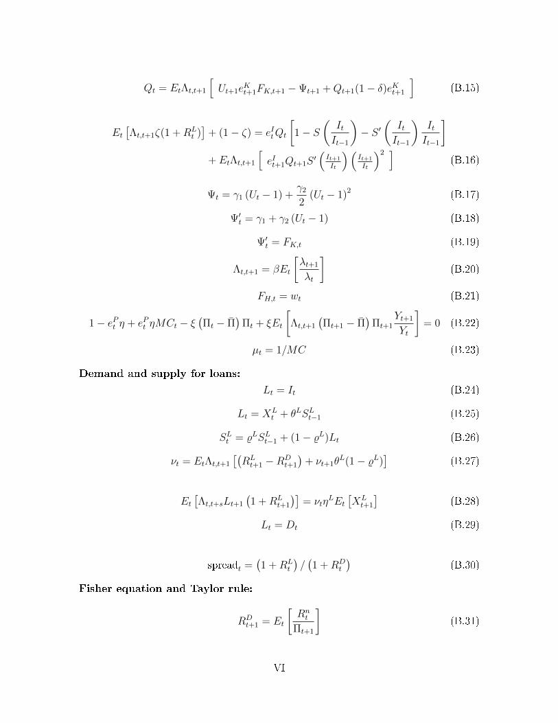
Qt = EtΛt,t+1

[Ut+1e

Kt+1FK,t+1 −Ψt+1 +Qt+1(1− δ)eKt+1

](B.15)

Et[Λt,t+1ζ(1 +RL

t )]

+ (1− ζ) = eItQt

[1− S

(ItIt−1

)− S ′

(ItIt−1

)ItIt−1

]+ EtΛt,t+1

[eIt+1Qt+1S

′(It+1

It

)(It+1

It

)2 ](B.16)

Ψt = γ1 (Ut − 1) +γ2

2(Ut − 1)2 (B.17)

Ψ′t = γ1 + γ2 (Ut − 1) (B.18)

Ψ′t = FK,t (B.19)

Λt,t+1 = βEt

[λt+1

λt

](B.20)

FH,t = wt (B.21)

1− ePt η + ePt ηMCt − ξ(Πt − Π

)Πt + ξEt

[Λt,t+1

(Πt+1 − Π

)Πt+1

Yt+1

Yt

]= 0 (B.22)

µt = 1/MC (B.23)

Demand and supply for loans:

Lt = It (B.24)

Lt = XLt + θLSLt−1 (B.25)

SLt = %LSLt−1 + (1− %L)Lt (B.26)

νt = EtΛt,t+1

[(RLt+1 −RD

t+1

)+ νt+1θ

L(1− %L)]

(B.27)

Et[Λt,t+sLt+1

(1 +RL

t+1

)]= νtη

LEt[XLt+1

](B.28)

Lt = Dt (B.29)

spreadt =(1 +RL

t

)/(1 +RD

t

)(B.30)

Fisher equation and Taylor rule:

RDt+1 = Et

[Rnt

Πt+1

](B.31)

VI

log

(Rnt

Rn

)= ρr log

(Rnt−1

Rn

)

+(1− ρr)

ρπ log(

Πt

Π

)+ ρy log

(YtY ft

)+ρ∆y

(log(YtY ft

)− log

(Yt−1

Y ft−1

))+ ρs log

(Lt

Lt−1Πt

)+ εRt , (B.32)

Resource constraint and exogenous processes:

Yt = Ct + It +Gt +ξ

2(Πt − 1)2 Yt +

ξW

2

(ΠWt − Π

)2WtHt + ΨtKt (B.33)

log

(eκteκ

)= ρκ log

(eκt−1

eκ

)+ εκt , κ = A,B,G, I, P,W,K (B.34)

C Steady state

K and H solve equations (B.27) and (B.3), evaluated at the steady state, while the

value of the remaining variables is found recursively by using the following relationships

Π = 1 (C.1)

ΠW = Π (C.2)

Λ = β (C.3)

U = 1 (C.4)

µW =η

η − 1(C.5)

MC =η − 1

η(C.6)

µ = 1/MC (C.7)

RD =1

β− 1 (C.8)

I = δK (C.9)

Y = HαK1−α (C.10)

G =G

YY (C.11)

VII

C = Y − I −G (C.12)

S = C (C.13)

X = (1− θ)C (C.14)

U =

[(X)φ (1−H)1−φ

]1−σc

1− σc(C.15)

UX = φ (1−H)1−φ[Xφ (1−H)1−φ

]−σcXφ−1 (C.16)

UH = − (1− φ) (1−H)−φXφ[Xφ (1−H)1−φ

]−σc(C.17)

W = µW (−UH/UX) (C.18)

L = ζI (C.19)

SL = L (C.20)

XL = (1− θL)L (C.21)

D = L (C.22)

FK =(1− α)

µ

Y

K(C.23)

R =β (FK + (1− ζ) (1− δ))− (1− ζ)

ζβ (1− β (1− δ))− 1 (C.24)

ν = ΛL(1 +RL

)/(ηLXL

)(C.25)

spread =(1 +RL

)/(1 +RD

)(C.26)

FH = W (C.27)

Q = Λ(1 +RL

)(C.28)

Ψ = 0 (C.29)

γ1 = FK (C.30)

Ψ′ = γ1 (C.31)

γ2 =γ1

σu(C.32)

S = S ′ = 0 (C.33)

VIII

D Data sources and transformations

This section discusses the sources of the eight observables used in the estimation and

their transformation. GDP, GDP deator ination, commercial and industrial loans of

all commercial banks, the federal funds rate, civilian population (CNP160V) and civil-

ian employment (CE160V) are downloaded from the FRED database of the Federal

Reserve Bank of St. Louis. Private consumption expenditures and xed private invest-

ment are extracted from the NIPA Table 1.1.5 of the Bureau of Economic Analysis. Av-

erage weekly hours worked (PRS85006023) and compensation per hour (PRS85006103)

are downloaded from the Bureau of Labor Statistics.

Data are transformed as in Smets and Wouters (2007). In particular, GDP, con-

sumption, investment and loans are transformed in real per-capita terms by dividing

their nominal values by the GDP deator and the civilian population. Real wages

are computed by dividing compensation per hour by the GDP deator. As shown in

the measurement equations in Subsection 3.1 of the paper, the observable variables

of GDP, consumption, investment, wages and loans are expressed in rst dierences.

Hours worked are multiplied by civilian employment, expressed in per-capita terms

and demeaned. The ination rate is computed as a quarter-on-quarter dierence of

the log of the GDP deator. The federal funds rate is expressed in quarterly terms

and the remaining variables are expressed as 100 times their logarithm. All series are

seasonally adjusted by their sources.

E Robustness of results to alternative Taylor rules

Figure E.1 reports prior and posterior probability densities of the parameters of the

alternative Taylor rules presented in Table 6 of the paper, and shows that ρs is identied

and positive in all cases.

Last, Tables E.1-E.4 show the parameter estimates of the alternative Taylor rules.

In the interest of brevity results on the estimation of alternative Taylor rules with

ρs = 0 are not reported but are available upon request.

IX

0.4 0.6 0.8 10

5

10

15

20

25

Int. rate smoothing, ρr

1 2 30

0.5

1

1.5

2

2.5

Response to inflation, ρπ

0 0.05 0.1 0.15 0.20

5

10

15

20

25

30

35

40

Response to output, ρy

−1 −0.5 0 0.5 10

1

2

3

4

5

6

7

Response to credit growth, ρs

(a) Implementable (I)

0.4 0.6 0.8 10

5

10

15

20

25

Int. rate smoothing, ρr

1 2 30

0.5

1

1.5

2

2.5


0 0.1 0.20

5

10

15

20

25

30

35

40

Response to output gap, ρy

0 0.1 0.2 0.30

2

4

6

8

10

Response to stock prices, ρq

−1 0 10

1

2

3

4

5

6

7


(b) Stock prices (II)

0 1 20

1

2

3

4

5

6

AR(1), ρ1

−2 −1 0 10

1

2

3

4

5

6

AR(2), ρ2

1 2 30

0.5

1

1.5

2

2.5


0 0.1 0.20

5

10

15

20

25

30

35

40


−1 0 10

1

2

3

4

5

6

7


(c) AR(2) smoothing (III)

0 1 20

1

2

3

4

5

6

AR(1), ρ1

−2 −1 0 10

1

2

3

4

5

6

AR(2), ρ2

1 2 30

0.5

1

1.5

2

2.5


0 0.1 0.20

5

10

15

20

25

30

35

40

45


0 0.1 0.2 0.30

2

4

6

8

10

Response to stock prices, ρq

−1 0 10

1

2

3

4

5

6

7


Prior density

Posterior density

(d) Stock prices and AR(2) smoothing (IV)

Figure E.1: Prior and posterior probability densities of parameters of alternative Taylorrules

X



Structural








Investment adjust. costs ψ Normal 4.00 1.50 3.2612 [0.7777;5.1334]






Averages





Exogenous processes


σA IG 0.10 2.0 0.0046 [0.0041;0.0052]


σG IG 0.10 2.0 0.0225 [0.0199;0.0249]



σI IG 0.10 2.0 0.0254 [0.0002;0.0454]


σB IG 0.10 2.0 0.0105 [0.0077;0.0132]


σK IG 0.10 2.0 0.0024 [0.0016;0.0032]


σP IG 0.10 2.0 0.0139 [0.0116;0.0162]


σW IG 0.10 2.0 0.0486 [0.0351;0.0599]



Table E.1: Prior and posterior distributions of the estimated parameters of the modelfeaturing an implementable Taylor-type rule augmented with credit growth (I) 90%condence intervals are in square brackets

XI



Structural














Stock prices-Taylor rule ρq Gamma 0.00 0.05 0.1497 [0.0502;0.2491]


Averages





Stock prices Q Normal 2.16 0.25 2.1551 [1.7742;2.5401]

Exogenous processes


σA IG 0.10 2.0 0.0047 [0.0041;0.0052]


σG IG 0.10 2.0 0.0224 [0.0197;0.0249]



σI IG 0.10 2.0 0.0259 [0.0002;0.0419]


σB IG 0.10 2.0 0.0101 [0.0075;0.0126]


σK IG 0.10 2.0 0.0024 [0.0016;0.0031]


σP IG 0.10 2.0 0.0140 [0.0114;0.0165]


σW IG 0.10 2.0 0.0507 [0.0371;0.0640]


Std measurement error stock prices σεQ IG 0.10 2.0 0.0755 [0.0668;0.0846]


Table E.2: Prior and posterior distributions of the estimated parameters of the modelfeaturing a Taylor-type rule augmented with credit growth and stock prices (II) 90%condence intervals are in square brackets

XII



Structural














Interest rate smoothing ρr Normal 1.10 0.50 1.3172 [1.2033;1.4381]

Interest rate smoothing order 2 ρr2 Normal -0.20 0.50 -0.4387 [-0.5531;-0.3270]

Averages




Hours of work h Normal 0.00 0.10 -0.0049 [-0.1629;0.1582]

Exogenous processes


σA IG 0.10 2.0 0.0046 [0.0041;0.0052]


σG IG 0.10 2.0 0.0225 [0.0198;0.0250]



σI IG 0.10 2.0 0.0302 [0.0133;0.0494]


σB IG 0.10 2.0 0.0107 [0.0076;0.0140]


σK IG 0.10 2.0 0.0029 [0.0018;0.0040]


σP IG 0.10 2.0 0.0138 [0.0115;0.0160]


σW IG 0.10 2.0 0.0473 [0.0337;0.0597]



Table E.3: Prior and posterior distributions of the estimated parameters of the modelfeaturing a Taylor-type rule augmented with credit growth and AR(2) interest ratesmoothing (III) 90% condence intervals are in square bracketsXIII



Structural














Stock prices-Taylor rule ρq Gamma 0.00 0.05 0.1136 [0.0319;0.1874]

Interest rate smoothing ρr Normal 1.10 0.50 1.2957 [1.789;1.4158]

Interest rate smoothing order 2 ρr2 Normal -0.20 0.50 -0.4141 [-0.5298;-0.3018]

Averages





Stock prices Q Normal 2.16 0.25 2.1568 [1.7734;2.5527]

Exogenous processes


σA IG 0.10 2.0 0.0047 [0.0041;0.0052]


σG IG 0.10 2.0 0.0224 [0.0198;0.0252]



σI IG 0.10 2.0 0.0258 [0.0003;0.0408]


σB IG 0.10 2.0 0.0107 [0.0078;0.0135]


σK IG 0.10 2.0 0.0030 [0.0020;0.0040]


σP IG 0.10 2.0 0.0141 [0.0117;0.0164]


σW IG 0.10 2.0 0.0471 [0.0336;0.0596]


Std measurement error stock prices σεQ IG 0.10 2.0 0.0759 [0.0667;0.0849]


Table E.4: Prior and posterior distributions of the estimated parameters of the modelfeaturing a Taylor-type rule augmented with credit growth, stock prices and AR(2)interest rate smoothing (IV) 90% condence intervals are in square brackets

XIV

St wr σr Pr(ZLB) ρr απ αy α∆y αs Ω ω

Optimized standard Taylor-type rules

20.0 0.402 0.006 1.000 0.572 0.000 0.000 -2.5246 -0.09

Optimized augmented Taylor-type rule

Lt/Lt−1 20.0 0.403 0.007 1.000 0.586 0.000 0.000 0.003 -2.5246 -0.09

Lt/L 20.0 0.410 0.007 1.000 0.544 0.000 0.000 0.003 -2.5246 -0.08spreadt/spread 20.0 0.405 0.007 1.000 0.573 0.000 0.000 -0.083 -2.5246 -0.09

Table F.1: Optimized alternative augmented monetary policy rules

F Robustness exercises for optimal policy

This section illustrates a series of modications in the DSGE model in order to investi-

gate the robustness of the optimal policy results to (i) Taylor-type rules augmented with

nancial variables alternative to nominal credit growth; (ii) implementable Taylor-type

rules; (iii) a higher volatility of structural shocks; and (iv) superinertial rules.

F.1 Alternative nancial variables

We rst report results on optimal policy when the augmented Taylor-type rule responds

to nancial variables dierent from nominal credit growth. We can write the Taylor

rule as

log

(Rnt

Rn

)= ρr log

(Rnt−1

Rn

)+ απ log

(Πt

Π

)+ αy log

(Yt

Y ft

)+ α∆y

[log

(Yt

Y ft

)− log

(Yt−1

Y ft−1

)]+ αs log (St) , (F.1)

where St is a nancial variable the monetary policy rate may react to. In particular,

we consider (i) real credit growth, Lt/Lt−1; (ii) the percent deviation of lending from its

steady state (Lt/L); and (iii) the bank spread, spreadt/spread ≡ (1+RLt )/(1+RD

t )/(1+RL)/(1+RD),

similarly to Curdia and Woodford (2010) and Aksoy et al. (2013).

Table F.1 shows that the optimal ρr , απ, αy and α∆y are similar to the ones under

the standard Taylor-type rule for the same wr = 20; hence, the welfare change, ω, is of

the same order of magnitude. This exercise unveils that if monetary policy responds to

real lending growth, deviation of lending from steady state or the deviation of spread

XV

from steady state, it achieves virtually the same welfare outcome as in the case of

nominal credit growth. The negative optimized coecient on spread is explained by

the fact that the model features a tight negative relationship between lending and this

variable.

F.2 Implementable Taylor-type rules

Table F.2 shows the optimized coecients in the case of the implementable Taylor-

type rule, equation (19) of the paper, which is reparametrized as follows:

log

(Rnt

Rn

)= ρr log

(Rnt−1

Rn

)+ απ log

(Πt

Π

)+ αy log

(YtY

)+ αs log

(LtLt−1

Πt

), (F.2)

where απ ≡ (1 − ρr)ρπ, αy ≡ (1 − ρr)ρy and αs ≡ (1 − ρr)ρs. Optimal policy results

are robust to this alternative formulation of the Taylor rule: the optimal responses

to output and to nominal credit growth are positive but small. In addition, the es-

timated implementable rule implies a consumption-equivalent welfare loss equal to

(0.54− 0.07) % = 0.47%, relative to the optimized rule with the same Pr (ZLB), ob-

tained setting wr = 10.5. Its order of magnitude is comparable to that of the baseline

Taylor-type rule.

Table F.2 also shows the optimal response to alternative nancial variables, St.These results are also robust to the alternative specication of the Taylor rule.

F.3 Highly volatile economy

The shocks used for the computation of optimized simple rules are those estimated

using data of the Great Moderation, characterized by low volatility of business cycle

uctuations. Therefore it seems appropriate to check whether the main results hold

in more turbulent periods characterized by higher volatilities. The Great Recession

witnessed a double standard deviation of real output growth compared to the average

level observed during the Great Moderation.

Figure F.1 presents a counterfactual experiment in which we proportionally change

the volatilities of all the structural shocks to match a standard deviation of output

double and triple compared to the baseline estimated model by keeping ρr , απ and

αy xed at their optimal values and by changing αs in the interval [0; 0.1]. The higher

XVI

wr σr Pr(ZLB) ρr απ αy αs Ω ω

Optimized standard implementable Taylor-type rules

0.0 1.002 0.164 0.610 3.000 0.011 -2.5243 0.00

20.0 0.404 0.007 1.000 0.569 0.001 -2.5246 -0.11

Optimized augmented implementable Taylor-type rule

11.5 0.469 0.017 1.000 0.787 0.004 0.005 -2.5245 -0.07

20.0 0.405 0.007 1.000 0.579 0.001 0.003 -2.5246 -0.11

Estimated implementable Taylor-type rule

0.468 0.017 0.857 0.288 0.003 0.050 -2.5258 -0.54

Optimized alternative augmented implementable Taylor-type rule

StLt/Lt−1 20.0 0.405 0.007 1.000 0.582 0.001 0.003 -2.52460 -0.11

Lt/L 20.0 0.411 0.007 1.000 0.544 0.000 0.003 -2.52460 -0.11

spreadt/spread 20.0 0.406 0.007 1.000 0.571 0.001 0.075 -2.52460 -0.11

Table F.2: Optimized implementable monetary policy rules

the standard deviation, the stronger is the trade-o between ination and nancial

stabilization. Hence the welfare loss is greater under the most volatile scenario and it

increases for a more aggressive responsiveness to nominal credit growth.

In order to highlight the importance of supply versus demand shocks in the design

of optimal policy, we then articially calibrate only the volatility of the capital quality

shock to match the higher standard deviation of output, keeping the volatilities of the

other shocks at their estimated values shown in Table 2 of the paper. This exogenous

disturbance is a demand shock, in which output, lending and ination move into the

same direction. Figure F.2 shows that it would be indeed optimal to lean against

windy bank lending, with an optimal αs around 0.05 in the higher volatility scenarios.

This result conrms that the source of business cycle uctuations is crucial for the

optimality of the leaning-against-the-wind policy.

XVII

0 0.01 0.02 0.03 0.04 0.05 0.06 0.07 0.08 0.09 0.10

0.1

0.2

0.3

0.4

0.5

0.6

Interest−rate responsiveness to nominal credit growth, αs

Welf

are c

ost, C

E los

s (%

)

Baseline STD

Double STD

Triple STD

Figure F.1: Welfare cost associated to leaning against the wind for proportional in-creases in the volatilities of all shocks (STD = standard deviation of real output growth)

0 0.01 0.02 0.03 0.04 0.05 0.06 0.07 0.08 0.09 0.1

−0.6

−0.5

−0.4

−0.3

−0.2

−0.1

0

Interest−rate responsiveness to nominal credit growth, αs

Welf

are c

ost, C

E los

s (%

)

Baseline STD

Double STD

Triple STD

Figure F.2: Welfare cost associated to leaning against the wind for larger volatilitiesof the capital quality shock (STD = standard deviation of real output growth)

F.4 Superinertial rules

The optimal policy results reported in the paper rule out the possibility that interest

rate inertia exceeds unity. In other words our optimized simple rules are not super-

inertial in the sense of Rotemberg and Woodford (1999) and Woodford (2003). Here

we check whether our conclusions remain unaltered when we allow for a ρr > 1. In

particular, Figure F.3 plots the welfare changes obtained (i) by letting inertia ρr and

the response to credit growth, αs, vary in the intervals [0, 2] and [0, 0.5], respectively,

and (ii) by re-optimizing the values of the remaining parameters in equation (23) in

the paper (απ, αy and α∆y). The welfare change is computed, relative to a reference

case of no inertia (ρr = 0) and no response to credit growth (αs = 0), in terms of the

consumption equivalent (CE) compensation that the representative agent should re-

XVIII

00.1

0.20.3

0.40.5

0

0.5

1

1.5

2−0.2

0

0.2

0.4

0.6

0.8

1

Response to credit growth, αs

Interest rate inertia, ρr

We

lfare

ch

an

ge

CE

(%

)

Figure F.3: Welfare change associated to interest rate inertia (ρr) and leaning againstthe wind (αs) relative to the case ρr = αs = 0

ceive to be as well o under the reference case as any other alternative regimes. Three

remarks are worth making from the inspection of the resulting surface. First, condi-

tional on αs = 0, raising ρr from zero to unity (price-level rule case) delivers a welfare

gain of around 0.7% in consumption-equivalent terms. Second, further increases in ρr

(superinertial rules) foster only negligible welfare changes, similarly to Schmitt-Grohe

and Uribe (2007). Third, the optimal value of αs is close to zero for every level of ρr,

hence higher values of αs are welfare-detrimental.

References

Aksoy, Y., Basso, H., and Coto-Martinez, J. (2013). Lending relationships and mone-

tary policy. Economic Inquiry, 51(1):368393.

Curdia, V. and Woodford, M. (2010). Credit spreads and monetary policy. Journal of

Money, Credit and Banking, 42(s1):335.

Rotemberg, J. J. and Woodford, M. (1999). Interest rate rules in an estimated sticky

price model. In Monetary policy rules, pages 57126. National Bureau of Economic

Research, Inc.

XIX

Schmitt-Grohe, S. and Uribe, M. (2007). Optimal simple and implementable monetary

and scal rules. Journal of Monetary Economics, 54(6):17021725.

Smets, F. and Wouters, R. (2007). Shocks and frictions in US business cycles: A

Bayesian DSGE approach. American Economic Review, 97(3):586606.

Woodford, M. (2003). Interest and prices: Foundations of a theory of monetary policy.

Princeton University Press.

XX

Leaning Against Windy Bank Lending

Documents

Transcript of Leaning Against Windy Bank Lending